JAIT

I.INTRODUCTION

Because of the wide existence of nonstationary signals, the time–frequency (TF) analysis methods on analyzing these signals, such as the short-time Fourier transform (STFT) [1], the Wigner-Ville distribution (WVD) [2], and the continuous wavelet transform (CWT) [3], have been developed for a long time. Much work has been done by a number of researchers, aiming to obtain the TF representation (TFR) with high TF resolution. In general, these methods can be divided into three categories, which are the basis-based TF analysis methods, the decomposition-based TF analysis method, and the post-processing methods.

For the basis-based TF analysis methods, it is necessary to construct the basis function in advance. Here, several classic basis-based methods are introduced. The STFT is a type of linear transform that employs a window function to truncate the raw nonstationary signal to obtain a series of truncated signals. By regarding these truncated signals as stationary signals and operating with Fourier transform on them, the TFR is obtained. For any piece of truncated signal, because we operate with Fourier transform on the product of the truncated signal and the window function, the chosen window function has a significant effect on the final TFR. Furthermore, the STFT is limited by the uncertainty principle, that is, we cannot obtain favorable time resolution and frequency resolution concurrently. One is acquired at the cost of the other necessarily. The WVD is a type of bilinear transform that does not need a window function to truncate the raw signal. Therefore, the WVD can inherently obtain a TFR with high resolution. However, because of its bilinear property, the TFR obtained using WVD is interfered by the illusive frequency components that generate from the crossing terms while analyzing multi-component signals, which limits the application of WVD to some extent. CWT is a type of TFR method whose wavelet basis is generated by mother wavelet and father wavelet, not the traditional Fourier basis. Different from STFT which uses the same window width in whole frequency domain, CWT can adaptively change the window width, that is, CWT uses the wide window width in low frequency range and narrow window width in high frequency range. By doing this, CWT can obtain a TFR with high TF resolution. However, its parameters are difficult to set. The chirplet transform (CT) is a type of method that aims to analyze the chirp-like signals, which obtain a TFR with high TF resolution by rotating the chirplets to match the instantaneous frequency (IF) of target signal to make it more stationary [4]. However, it is only suitable for the mono-component signals with linear IF. To improve the limitations of the above methods, researchers have done a lot of work. In order to improve the STFT, STFT with adaptive window width based on the chirp rate (ASTFT) was proposed by adopting adaptive widow width [5,6]. By making the standard deviation of the Gaussian window function be a function of time and frequency instead of an unchanged parameter in traditional STFT, the window width in the ASTFT can adaptively vary with time and frequency. Hence, ASTFT can obtain different TF resolution at different time and frequency points. Although ASTFT can improve the TF resolution to some extent, its parameters are difficult to set. Furthermore, because it does not improve the parameter for window size, the inherent limitation resulted from the uncertainty principle remains. In order to improve the WVD, the pseudo-WVD (PWVD) was proposed to restrain the crossing terms by adding window function in time and frequency domain [7]. Although the PWVD improves the bad effect of crossing terms to some extent, this limitation is still not solved because of the bilinear property of WVD. Furthermore, the inherently high TF resolution is lost due to the added window function. In order to improve the CT, many extending methods are proposed. To expand the application scope, the polynomial CT (PCT) was proposed to analyze the signals with nonlinear IF using polynomial kernel to replace the linear kernel in tradition CT [8]. However, if the IF of target signal cannot be fitted by polynomial, the PCT is not effective. Therefore, the spline-kernel CT (SCT) was proposed using splined kernel, which can be suitable for any complex IF [9]. However, PCT and SCT can only adapt to mono-component signals. To make CT suitable for multi-component signals, general linear CT (GLCT) was proposed [10]. GLCT obtains a TFR with high TF resolution by generating a series of sub-TFRs and fusing them into one. Because fusing rule is to choose the maximum in all sub-TFRs at each time and frequency center in whole TF plane, it inevitably produces the fake frequency components. Furthermore, the smaller the frequency interval between adjacent frequency component, the more serious the illusive frequency component. To improve the smear effect, the velocity synchronous linear CT (VSLCT) was proposed by constructing the basis according to the rotating speed to make the chirplets match the IFs better [11]. In this way, VSLCT can obtain a TFR with high TF resolution. It is a good idea to vitiate the bad effect of the uncertainty principle by utilizing an adaptive window size. However, it performs not very well on analyzing the signals with the crossing IFs.

For the decomposition-based methods, the core idea of these methods is to decompose the multi-component signal into a series of mono-component signals without constructing basis function in advance. Here, several decomposition methods are introduced. Hilbert–Huang transform as well as the improved methods, such as ensemble empirical mode decomposition [12] and ensemble local mean decomposition [13], is a type of classic decomposition method [14], which needs no prior knowledge. However, it is only suitable for the signals whose IF varies with time slowly. Mode mixing is serious while analyzing the signals whose IF varies with time violently. Adaptive iterative generalized demodulation method is a type of decomposition-based method using surrogate test to decompose the multi-component signal [15]. It needs prior knowledge in advance, for example, the changing trend of IF with time. Furthermore, when the signals contain too many frequency components, it is not efficient. The variational nonlinear chirp mode decomposition is another type of decomposition-based method that considers the target signals as a whole and does not separate the sub-components successively [16]. Although its corresponding decomposition is efficient, it not only needs the number of frequency components in advance but also the changing trend with time for all frequency components to assign initial iterative values.

For the post-processing methods, such as reassignment method [17], synchro-extracting method [18], and synchro-squeezed wavelet transform [19], their performance mainly depends on the original TFR obtained by traditional methods, such as STFT and CWT. It is worth to mention that post-processing methods can obtain a TFR with high TF resolution, when traditional methods can obtain relatively nice results. However, if the TFR obtained by traditional methods is not in a favorable level, the results obtained using post-processing methods are not satisfying as well. Furthermore, for the signal with crossing IFs, there exists signal distortion at the intersection of IFs in the TFR obtained using post-processing methods.

In this paper, we propose a novel TF analysis method called OSTFT by replacing the even symmetric window function with odd symmetric function. By acquiring minimum amplitude of 0 at time and frequency center, OSTFT can obtain a TFR with high TF resolution. Different from the TFR obtained using STFT whose TF resolution deteriorates because of the energy leakage, the TFR obtained using OSTFT acquires high TF resolution by utilizing energy leakage. In addition, it is worth to mention that the proposed OSTFT can vitiate the effect of window size that we choose on the TFR obtained. Furthermore, it has a nice performance on the special signals, for example, the signals with crossing IFs. The effectiveness of OSTFT has been validated on two numerical signals with complex IFs and an experimental signal collected from a brown bat [20].

The rest of paper is structured as follows: A succinct description of the main limitation of windowed transforms and a detailed discussion of the proposed OSTFT are provided in Section II, the effectiveness of the proposed method is examined using numerical signals and an experiment signal in Section III and IV-A, respectively, a discussion part is displayed in Section IV-B, and the conclusions that can be drawn from this study are presented in Section V.

II.OSTFT

A.LIMITATION OF WINDOWED TRANSFORM

In this subsection, we begin our study with uncertainty principle limiting the performance of windowed transform, which is given as follows:

E_{x} = {\int | x (t) |}^{2} d t = {\int | X (ω) |}^{2} d ω

(1)

where x(t) is a certain signal, X(ω) is the Fourier transform (FT) of x(t), and E_x is the energy of signal x(t).

{\begin{cases} t_{c} = \frac{1}{E_{x}} \int t {| x (t) |}^{2} d t \\ ω_{c} = \frac{1}{E_{x}} \int ω {| X (ω) |}^{2} d ω \end{cases}

(2)

where t_c is time center and ω_c is the frequency center.

{\begin{cases} {σ_{t}}^{2} = \frac{1}{E_{x}} \int {(t - t_{c})}^{2} {| x (t) |}^{2} d t \\ {σ_{ω}}^{2} = \frac{1}{E_{x}} \int {(ω - ω_{c})}^{2} {| X (ω) |}^{2} d ω \end{cases}

(3)

where σ_t is the time bandwidth and σ_ω is the frequency bandwidth.

By calculations, we can obtain

σ_{t} σ_{ω} \geq 1 / 2

(4)

According to (4), we know that the time resolution and frequency resolution cannot obtain the best levels concurrently, that is, one achieves a high level at the cost of the other necessarily. Among most of applications, we always hope that high frequency resolution is obtained to recognize the significant frequency component. However, because of the nonstationarity of nonstationary signal, we analyze a series of windowed signals in a short time using a window function to truncate the raw signal. Therefore, high frequency resolution is difficult to obtain under this condition. Furthermore, it is worthy of mentioning that the bad resolution is shown as the form of energy leakage. Here, we use a numerical signal with a sampling frequency of 200 Hz to present it further, which is constructed as the following expressions:

x_{1} (t) = \sin (2 π \int v (t) d t)

(5)

where v(t) is the IF, which is given as follows:

v (t) = - 18 t^{2} + 72 t + 18

(6)

In this case, we use STFT with window size of 128 to analyze this signal, whose corresponding analyzing results are shown in Fig. 1. Figure 1(a) shows the resulting TFR. Here, we take the time center at 1 s as an example. As per (6), the true IF at 1 s is 72 Hz. By observing Fig. 1(a), it can be seen that the leaked energy distributes in a range from $72 - Δ f$ to $72 + Δ f$ , where $Δ f$ is a certain frequency interval. The amplitude spectrum at 1 s shown in Fig. 1(b) presents the same results clearly.

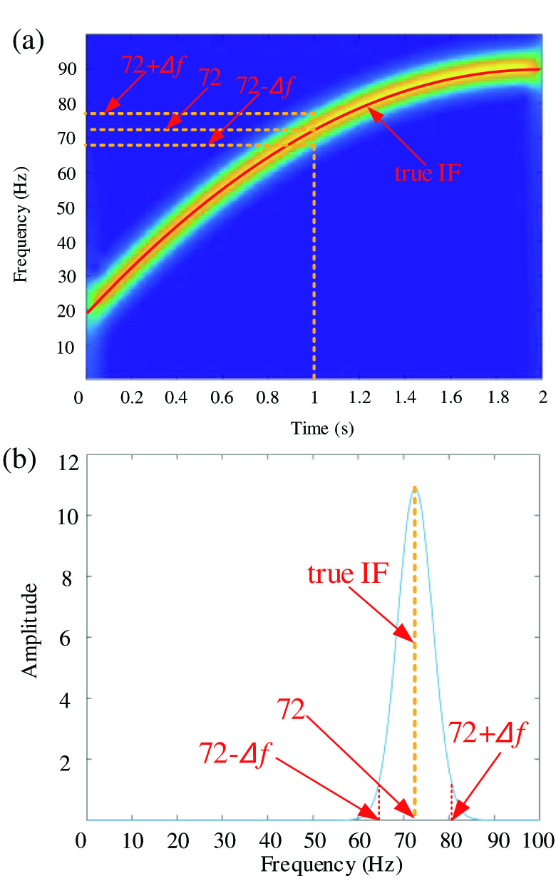Fig. 1. Analyzing results of x1(t): (a) TFR using STFT and (b) amplitude spectrum at time center of 1 s.

According to the above analysis, we can find that the leaked energy leads to the TFR with bad TF resolution. And in this paper, we mainly aim to resolve this problem to obtain a TFR with high TF resolution.

B.REVIEW OF STFT

In this subsection, we take the STFT as an example. By in-depth analysis of STFT, we can know the reason why STFT cannot obtain a TFR with high TF resolution. The STFT of a signal $s (u) \in L^{2} (R)$ is represented as the following expression:

{STFT}_{s} (t_{c}, ω_{c}) = \int_{- \infty}^{+ \infty} s (u) g (u - t) \exp (- j ω_{c} u) d u

(7)

where

t_{c} \in R

is the time center,

ω_{c} \in R

is the frequency center, j denotes

\sqrt{- 1}

; and g denotes window function which is usually taken as Gaussian function, which is represented as the following expression:

g_{σ} (u) = \frac{1}{\sqrt{2 π} σ} \exp (- \frac{1}{2} {(\frac{u}{σ})}^{2})

(8)

where σ is the standard deviation.

Because STFT is a windowed transform, it can be explained in a single window. Therefore, we can obtain

{STFT}_{s, t_{c}} (t_{c}, ω) = \int_{t_{c} - Δ}^{t_{c} + Δ} s (u) g (u - t_{c}) \exp (- j ω u) d u

(9)

where t_c is the time center of a certain window and

Δ

is the half window length.

To clearly present our core idea, we first regard s(u), in (9), as a mono-component signal with IF of v(u). In a certain window (a short time), based on Taylor’s theorem, v(u) can be represented as

v (u) \approx v (t_{c}) + v^{'} (t_{c}) (u - t_{c}) u \in (t_{c} - Δ, t_{c} + Δ)

(10)

where v(t_c) is the IF at time center t_c; v′(t_c) is the first-order derivative of v(u) at time center t_c, and the remainder is ignored.

According to (10), the phase function of s(u) in a certain window is obtained, which is given as the following expression:

ϕ (u) = v (t_{c}) u + \frac{v^{'} (t_{c})}{2} {(u - t_{c})}^{2}

(11)

Hence, s(u) can be represented as the following equivalent form:

s (u) = A (u) \cos (ϕ (u))

(12)

where A(u) is the instantaneous amplitude and φ(u) is the instantaneous phase.

According to Euler’s formula, (12) can be written as the following expression:

s (u) = A (u) \frac{e^{j ϕ (u)} + e^{- j ϕ (u)}}{2}

(13)

Substituting (11) into (13) produces

s (u) = A (u) \frac{e^{j (v (t_{c}) u + v^{'} (t_{c}) {(u - t_{c})}^{2} / 2)} + e^{- j (v (t_{c}) u + v^{'} (t_{c}) {(u - t_{c})}^{2} / 2)}}{2}

(14)

For the sake of the convenience in next deduction, we take some mathematical skills as follows:

s (u) = s_{1} (u) + s_{2} (u)

(15)

s_{1} (u) = A (u) e^{j (v (t_{c}) u + v^{'} (t_{c}) {(u - t_{c})}^{2} / 2)} / 2

(16)

s_{1 o} (u) = A (u) e^{j (v^{'} (t_{c}) u^{2} / 2)} / 2

(17)

s_{2} (u) = A (u) e^{- j (v (t_{c}) u + v^{'} (t_{c}) {(u - t_{c})}^{2} / 2)} / 2

(18)

s_{2 o} (u) = A (u) e^{- j (v^{'} (t_{c}) u^{2} / 2)} / 2

(19)

Here, the reason why STFT cannot achieve a pretty favorable TFR for nonstationary signals is uncovered. According to the convolution transform [21], (9) can be written in the following form:

{STFT}_{s, t_{c}} (t_{c}, ω) = \frac{1}{2 π} {FT}_{s} (ω) * {FT}_{g (u - t_{c})} (ω)

(20)

where * denotes convolution calculation, FT denotes Fourier transform, and

{FT}_{s} (ω) = \int_{t_{c} - Δ}^{t_{c} + Δ} s (u) \exp (- j ω u) d u

(21)

{FT}_{g (u - t_{c})} (ω) = \int_{t_{c} - Δ}^{t_{c} + Δ} g (u - t_{c}) \exp (- j ω u) d u

(22)

According to (15), (16), and (18), based on the linear property of FT, we can obtain

{FT}_{s} (ω) = {FT}_{s 1} (ω) + {FT}_{s 2} (ω)

(23)

where s1 is (16) and s2 is (18).

Substituting (23) into (20) produces

{STFT}_{s, t_{c}} (t_{c}, ω) = \frac{1}{2 π} ({FT}_{s 1} (ω) + {FT}_{s 2} (ω)) * {FT}_{g (u - t_{c})} (ω)

(24)

Here, we first only consider the FT_s1(ω) in (24). According to time and frequency shifting properties of FT, we can obtain

{FT}_{s 1} (ω) = {FT}_{s_{1 o}} (ω - v (t_{c})) \exp (- j ω t_{c})

(25)

{FT}_{g (u - t_{c})} (ω) = {FT}_{g (u)} (ω) \exp (- j ω t_{c})

(26)

where s_1o is (17) and g(u) is (8).

According to (24), (25), and (26), we can obtain

{STFT}_{s 1, t_{c}} (t_{c}, ω) = \frac{1}{2 π} (\begin{matrix} {FT}_{s_{1 o}} (ω - v (t_{c})) \dots \\ {* FT}_{g (u)} (ω) \end{matrix}) \exp (- j ω t_{c})

(27)

where s1 is (16) and s_1o is (17).

According to (27), we can obtain

| {STFT}_{s 1, t_{c}} (t_{c}, ω) | = | \frac{1}{2 π} {FT}_{s_{1 o}} (ω - v (t_{c})) * {FT}_{g (u)} (ω) |

(28)

Carrying out the same operations as FT_s1(ω), we can get the similar result of FT_s2(ω) in (24).

| {STFT}_{s 2, t_{c}} (t_{c}, ω) | = | \frac{1}{2 π} {FT}_{s_{2 o}} (ω + v (t_{c})) * {FT}_{g (u)} (ω) |

(29)

Because ${FT}_{g (u)} (ω)$ , ${FT}_{s_{1 o}} (ω - v (t_{c}))$ , and ${FT}_{s_{2 o}} (ω + v (t_{c}))$ are even symmetric functions with symmetric axes of ω=0, ω=v(t_c), and ω=-v(t_c), respectively, $| {STFT}_{s 1} (t_{c}, ω) |$ and $| {STFT}_{s 2} (t_{c}, ω) |$ are even symmetric functions with symmetric axes of ω=v(t_c) and ω=-v(t_c), respectively. And $| {STFT}_{{s, t}_{c}} (t_{c}, ω) |$ is composed by both two parts as shown in Fig. 2 clearly. The result shown in Fig. 2 is in accordance with the result shown in Fig. 1.

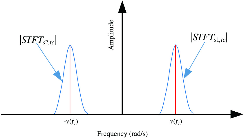Fig. 2. Amplitude spectrum of s(u) obtained using STFT at time center tc.

The above analysis mainly aims to explain mono-component signals. As for the multi-component signal, we can regard it as the summation of its every frequency component, which is represented as

s_{multi} (t) = \sum_{i = 1}^{n} s_{mono, i} (t)

(30)

where n is the number of intrinsic mode functions, and s_mono,I is the i^th intrinsic mode function.

Based on the linear property of FT, the FT of s_multi is the summation of FT of s_mono,i. Therefore, the above explanation results of the mono-component signal are suitable for the multi-component signal as well.

By observing (28) and (29), we can find that the $| {STFT}_{s 1, t_{c}} (t_{c}, ω) |$ and $| {STFT}_{s 2, t_{c}} (t_{c}, ω) |$ mainly depend on ${FT}_{g (u)} (ω)$ , the FT of window function. And among nearly all windowed transforms, the even symmetric window function is employed, which inevitably leads to energy leakage resulting in TFR with bad TF resolution. Aiming to resolve this problem, we propose a novel algorithm called the OSTFT, whose detailed explanations are shown in Section II-C.

C.PROPOSED OSTFT APPROACH

To resolve the above problem, completely different from conventional TF analysis methods employing the even symmetric window function, we employ the odd symmetric window function. It is worthy of mentioning that the proposed method aims not to restrain the leaked energy but to utilize it. By doing this, OSTFT can obtain a TFR with high TF resolution. This idea is suitable for all TF analysis methods based on FT. Here, we still take STFT as an example.

There exist many suitable odd symmetric window functions. However, in this study, we take a constructed window function called Gaussian-like window function (GL-window function), which is presented as the following expression:

l (t) = a u \exp (- b^{2} u^{2})

(31)

where a and b are positive parameters, respectively. In this study, a and b are taken as 200 and 10, respectively.

According to (31), we can obtain the FT of l(t),

{FT}_{l} (ω) = - \frac{a \sqrt{π}}{b^{2}} \frac{j ω}{2} e^{{(\frac{j ω}{2})}^{2}}

(32)

By observing (31) and (32), it can be seen that FT_l(ω) has the same expression as l(t).

Here, replacing g(u-t_c) with l(u-t_c) in (9) produces

{OSTFT}_{s, t_{c}} (t_{c}, ω) = \int_{t_{c} - Δ}^{t_{c} + Δ} s (u) l (u - t_{c}) \exp (- j ω u) d u

(33)

where l(u-t_c) is an odd symmetric function with symmetric center (t_c, 0).

In addition, FT of l(u-t_c) can also be calculated, which is given as follows:

{FT}_{l (u - t_{c})} (ω) = {FT}_{l (u)} (ω) \exp (- j ω t_{c})

(34)

where l(u) is (31) with symmetric center (0, 0).

By the similar deductions shown in Section II-B, we can obtain the results with similar expression like (27) for OSTFT,

{OSTFT}_{s 1, t_{c}} (t_{c}, ω) = \frac{1}{2 π} (\begin{matrix} {FT}_{s_{1 o}} (ω - v (t_{c})) \dots \\ * {FT}_{l (u)} (ω) \end{matrix}) \exp (- j ω t_{c})

(35)

{OSTFT}_{s 2, t_{c}} (t_{c}, ω) = \frac{1}{2 π} (\begin{matrix} {FT}_{s_{2 o}} (ω - v (t_{c})) \dots \\ * {FT}_{l (u)} (ω) \end{matrix}) \exp (- j ω t_{c})

(36)

where s1 is (16), s_1o is (17), s2 is (18), s_2o is (19), and l(u) is (31).

Based on (35) and (36), we can obtain

| {OSTFT}_{s 1, t_{c}} (t_{c}, ω) | = | \frac{1}{2 π} {FT}_{s_{1 o}} (ω - v (t_{c})) * {FT}_{l (u)} (ω) |

(37)

| {OSTFT}_{s 2, t_{c}} (t_{c}, ω) | = | \frac{1}{2 π} {FT}_{s_{2 o}} (ω + v (t_{c})) * {FT}_{l (u)} (ω) |

(38)

Because ${FT}_{s_{1 o}} (ω - v (t_{c}))$ and ${FT}_{s_{2 o}} (ω + v (t_{c}))$ are even symmetric functions with symmetric axes ω=v(t_c) and ω=−v(t_c), respectively, and ${FT}_{l (u)} (ω)$ is an odd function, ${OSTFT}_{s 1, t_{c}} (t_{c}, ω)$ and ${OSTFT}_{s 2, t_{c}} (t_{c}, ω)$ are odd symmetric functions with symmetric centers (v(t_c), 0) and (−v(t_c), 0), respectively. Hence, $| {OSTFT}_{s 1, t_{c}} (t_{c}, ω) |$ and $| {OSTFT}_{s 2, t_{c}} (t_{c}, ω) |$ are still even symmetric functions with symmetric axes ω=v(t_c) and ω=−v(t_c), respectively. But, completely different from conventional STFT whose amplitude functions, shown in (28) and (29), acquire maximums at ω=v(t_c) and ω=−v(t_c), respectively, the amplitude functions using OSTFT, shown in (37) and (38), acquire minimums of 0 at ω=v(t_c) and ω=−v(t_c), respectively, as shown clearly in Fig. 3. In this way, the TFR obtained using OSTFT can obtain the high TF resolution.

Fig. 3. Amplitude spectrum of s(u) obtained using OSTFT at time center tc.

Here, we still use the signal of x₁(t) to further explain the idea of OSTFT. The parameter for window size is set to 128. And the corresponding analyzing results are shown in Fig. 4. Figure 4(a) shows the TFR using OSTFT. According to Fig. 4(a), it can be seen that OSTFT can obtain a TFR with quite high TF resolution by utilizing the leaked energy. Furthermore, the estimated IF is nearly overlapped with the true IF. Figure 4(b) shows the amplitude spectrum at 1 s. From Fig. 4(b), the result is perfectly in accordance with the result shown in Fig. 3.

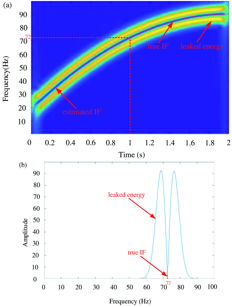Fig. 4. Analyzing results of x1(t) using OSTFT: (a) TFR and (b) amplitude spectrum at 1 s.

In fact, if the peak of each IF curve of the TFR using STFT can be well extracted, they are extremely close to the curves obtained by OSTFT. However, these curves should be extracted manually. The IF curves of the TFR of OSTFT can be easily contained because they are zeros in the TFR.

III.SIMULATION EVALUTION

In this section, two simulated numerical signals with complex IFs are employed to verify the performance of OSTFT.

A.CASE 1

In this subsection, the first multi-component signal with complex IFs is used to evaluate the performance of OSTFT, which is constructed as the following expression:

x_{2} (t) = \sum_{i = 1}^{3} 3 \cos (2 π \int_{0}^{t} v_{i} (u) d u)

(39)

where

{\begin{cases} v_{1} (u) = 70 \\ v_{2} (u) = 370 - 150 \sin (6 π u) - 50 \cos (4 π u) \\ v_{3} (u) = - 480 u^{2} + 480 u + 600 \end{cases}

(40)

The corresponding analyzing results are displayed in Fig. 5. Figure 5(a) and (b) shows the waveform with sampling rate of 1·8 kHz and the corresponding IFs, respectively. TFRs obtained using STFT and OSTFT with window size of 128 are shown in Fig. 5(c) and (e). According to Fig. 5(c), because of relatively serious energy leakage, the TFR obtained using STFT cannot obtain the high TF resolution. However, the TFR obtained using OSTFT shown in Fig. 5(e) shows sharp IF trajectories, which proves that OSTFT can obtain the TFR with high TF resolution. By observing estimated IFs (red curves) and true IFs (black curves) in Fig. 5(d), it can be seen that estimated IFs can track true IFs very well. Hence, the value of the Error is low. It proves that OSTFT can acquire satisfactory accuracy, even for this kind of complex signal.

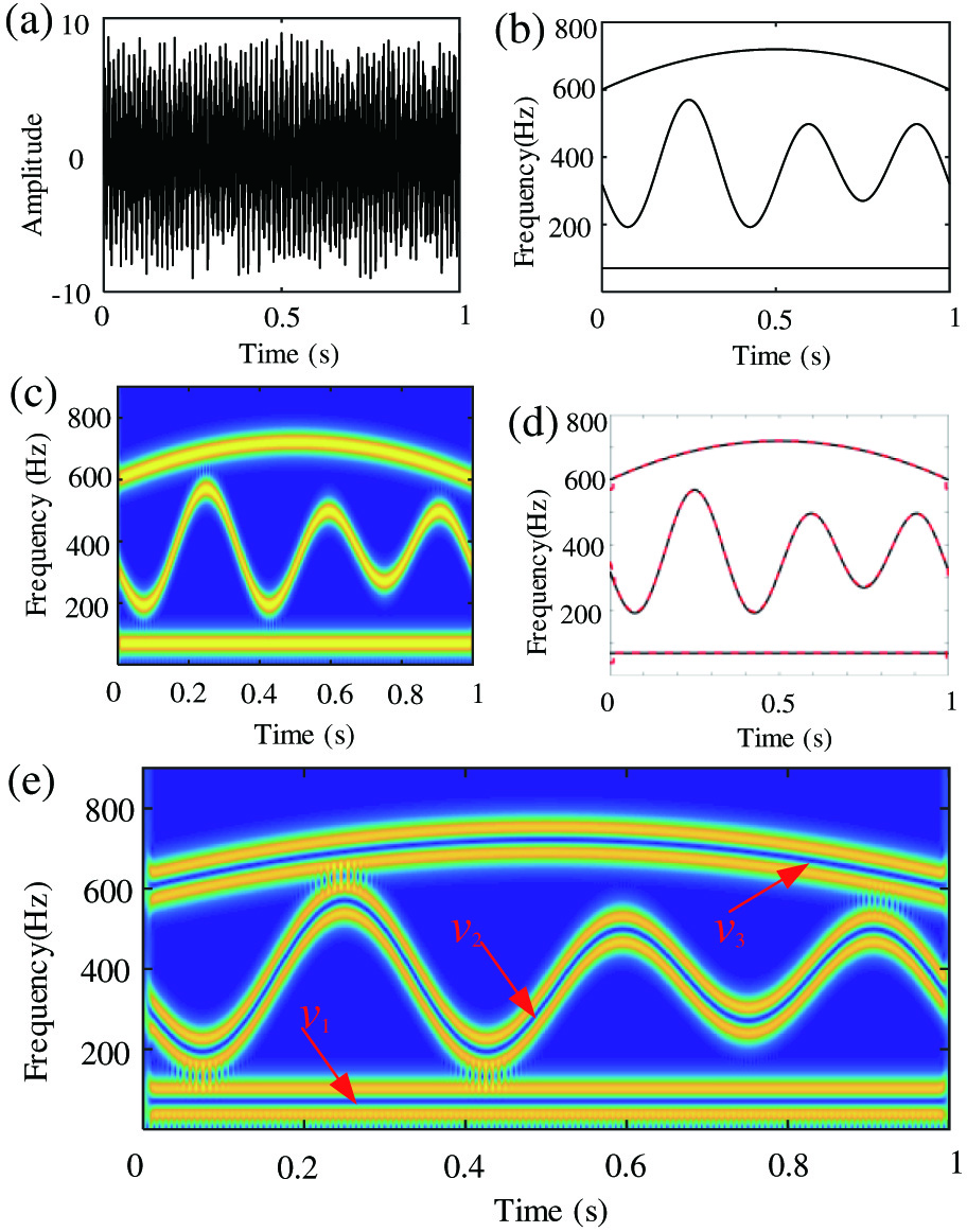Fig. 5. Analyzing results of signal x2: (a) waveform, (b) IFs, (c) TFR obtained using STFT, (d) estimated IFs (red curve) and true IFs (black curve), and (e) TFR obtained using OSTFT.

B.CASE 2

In this subsection, the other numerical signal with crossing IFs is constructed to evaluate the ability of OSTFT in analyzing special signals, which is constructed as the following expression:

x_{3} (t) = \sum_{i = 1}^{2} \sin (2 π \int_{0}^{t} v_{i} (u) d u)

(41)

where

{\begin{cases} v_{1} (u) = 25 - 5 \cos (u) \\ v_{2} (u) = 25 + 15 \cos (u) \end{cases}

(42)

The corresponding analyzing results are displayed in Fig. 6. Figure 6(a) and (b) shows the waveform with sampling rate of 100 Hz and the corresponding IFs, respectively. TFRs obtained using STFT and OSTFT with window size of 128 are displayed in Fig. 6(c) and (d), respectively. According to Fig. 6(c), TFR obtained using STFT is very blurred, which leads to bad TF resolution. Furthermore, because of the relatively energy leakage, it is difficult to determine whether the IFs are truly intersected or not. However, from the TFR obtained using OSTFT, shown in Fig. 6(d), the IF trajectories in the TFR are clear, sharp, and accurate by comparing with true IFs in Fig. 6(b). Furthermore, according to Fig. 6(d), it can be seen that the TFR using OSTFT can not only acquire the high TF resolution but also show the intersection of the IFs shown in the red square can be captured accurately.

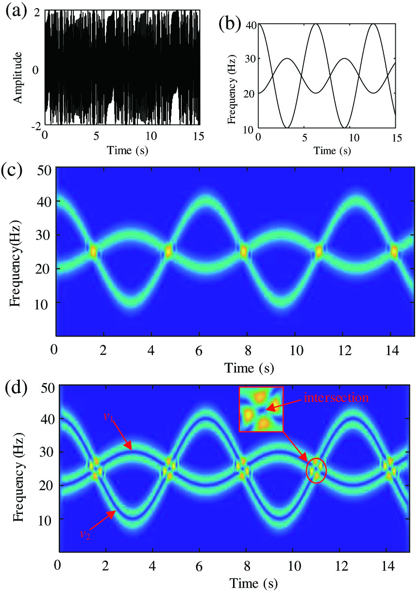Fig. 6. Analyzing results of x3(t): (a) waveform, (b) IFs, (c) TFR obtained using STFT, and (d) TFR obtained using OSTFT.

Through the above analysis, we can know that, even for this type of special signal, OSTFT can have a favorable performance.

Based on the above analysis of two cases, OSTFT can acquire TFR with pretty satisfying TF resolution for multi-component signals with not only complex IFs but also crossing IFs, which cannot be well resolved by traditional STFT.

IV.EXPERIMENT

In this section, an echolocation signal emitted by a large brown bat collected from real life is employed to test the effectiveness of OSTFT in Section A. Furthermore, two significant points about OSTFT are discussed in Section B.

A.EXPERIMENTAL CASE 1

In this subsection, the signal collected from a brown bat is analyzed using OSTFT, which is a multi-component signal with four time-varying IFs. STFT is chosen as a comparison method. In this case, the parameter for window size is set to 128 for both methods. The corresponding analyzing results are displayed in Fig. 7. Figure 7(a) shows the waveform with sampling period of 7 μs. TFRs obtained using STFT and OSTFT are shown in Fig. 7(b) and (c), respectively. According to Fig. 7(b), we can find that IF trajectories in the TFR obtained using STFT are blurred, resulting in bad TF resolution. However, IF trajectories, deep blue curves indicated by red arrows shown in Fig. 7(c), are very clear and sharp, which proves that OSTFT can acquire a TFR with high TF resolution by utilizing the leaked energy. By the above analysis, it can be seen that OSTFT has a good performance on obtaining a TFR with a high TF resolution.

Fig. 7. Analyzing results of signal collected from brown bat: (a) waveform, (b) TFR obtained using STFT, and (c) TFR obtained using OSTFT.

B.EXPERIMENTAL CASE 2

As rotation machineries become increasingly complex, TF analysis methods are an effective tool to diagnose faults in the machinery. A vibration signal collected from a water turbine is analyzed here. The sampling frequency of this signal is 16 Hz, and the number of sampling points is 1024. Figure 8(a) and (b) shows the corresponding waveform and rotation frequency, respectively. Then, the STFT and OSTFT are used for comparison. Figure 8(c) and (d) shows that the TFR is composed of several harmonics with regard to the rotation frequency; these harmonics can reveal the health condition of the water turbine.

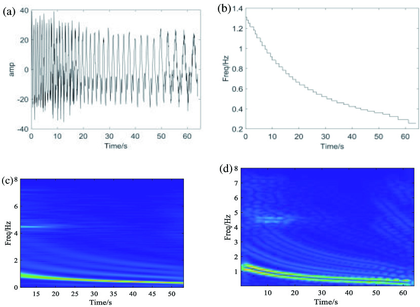Fig. 8. Vibration signal and TFRs of a water turbine: (a) waveform and (b) rotation frequency, (c) TFR obtained using STFT, and (d) TFR obtained using OSTFT.

It can be seen that more harmonics with higher resolution can be found in Fig. 8(d) compared with the STFT-based TFR shown in Fig. 8(c).

C.DISCUSSION

In this subsection, we mainly discuss two important issues. One is the effect of the parameter for window size we choose on the TFR obtained using OSTFT. The other is about the amplitude information at time and frequency centers ignored by OSTFT.

Firstly, we discuss the first significant issue. Based on the analysis in Section II, because the window function has a main effect on the energy leakage, and the OSTFT acquires the minimums of 0 at the time and frequency center, we can know that the TFR obtained using OSTFT is not sensitive to the window size, that is, the OSTFT vitiates the effect of window size on the TFR obtained. Here, we still use the numerical signal x₂(t) to further explain it. The sampling rate of x₂(t) is 1800 Hz, which lasts for 1 s. Hence, the total size of data points is 1800. Here, we use the OSTFT to analyze this signal by setting different window sizes as 100 and 300, respectively. The latter window size is three times as large as the former. In this case, we still take the STFT as a comparison method. The corresponding analyzing results are displayed in Fig. 9. By comparing TFRs obtained using STFT with window size of 100 and 300, respectively, as shown in Fig. 9(a) and (c), we can find that this parameter for window size has a serious effect on the TFRs. Furthermore, the larger the window size, the relatively higher the TF resolution. Although the large window size can help to acquire a relatively high TF resolution, it is not suitable for strong nonstationary signals. As shown in Fig. 9(c), the IF trajectory of v₂ is more blurred than that of v₁, because of their different levels of nonstationarity. However, through comparing Fig. 9(b) and (d), we can find that the TFRs obtained using OSTFT can acquire high TF resolution, whether the window size is set as 100 or 300. Furthermore, according to TFRs obtained using OSTFT, it can be also seen that the parameter for window size only has an effect on leaked energy. By the above analysis, we can know that OSTFT can vitiate the effect of window size on TFR obtained.

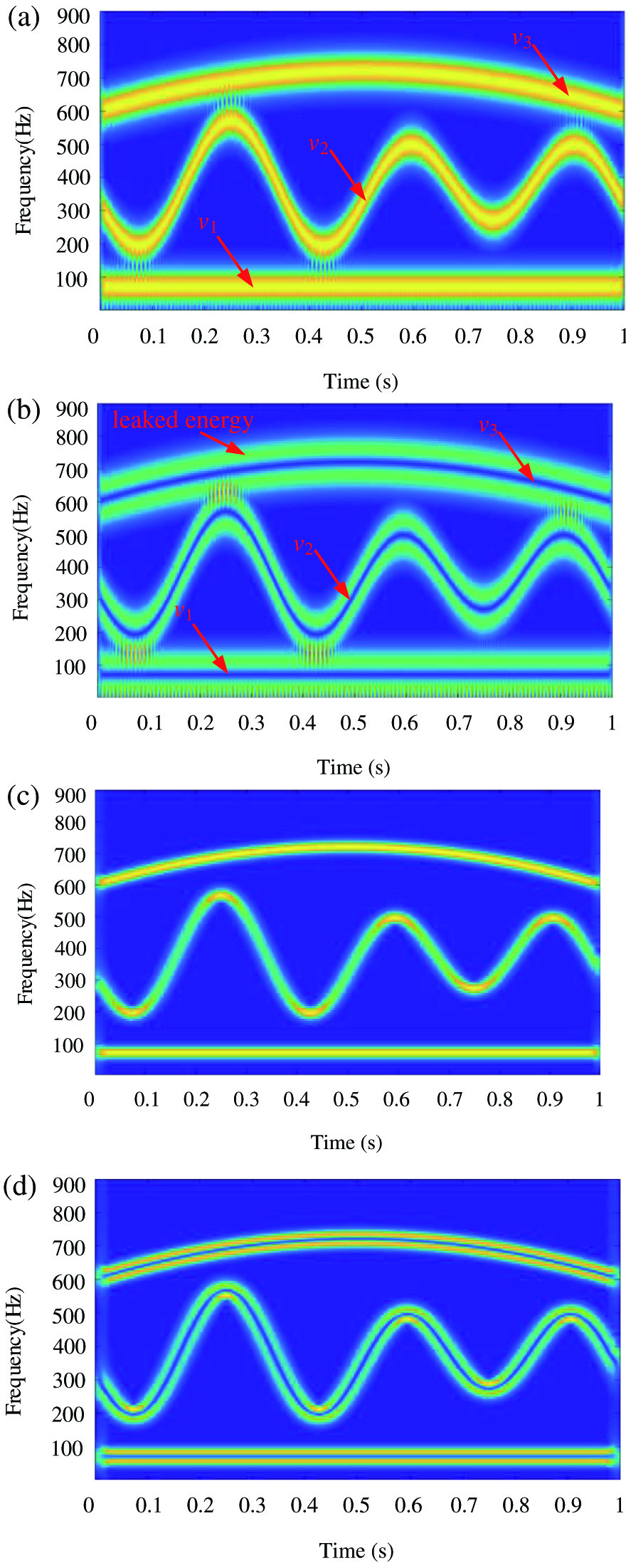Fig. 9. Analyzing results for the first significant point: (a) TFR obtained using STFT with window size 100, (b) TFR obtained using OSTFT with window size 100, (c) TFR obtained using STFT with window size 300, and (d) TFR obtained using OSTFT with window size 300.

Secondly, we discuss the other significant point. According to the analysis shown in Section II-C, the OSTFT inevitably ignores the amplitude information at time and frequency centers, because OSTFT acquires the minimums of 0 at time and frequency centers in the TF plane. Although the OSTFT loses the amplitude information at time and frequency centers, the amplitude changing trend of different frequency components can be obtained according to that of leaked energy. Here, we construct a numerical signal similar with x₂(t) to further explain it by changing the coefficients of different intrinsic modes of x₂(t). And the rest of parameters of x₂(t) remain unchanged. The constructed signal is given as the following expression:

x_{4} (t) = \sum_{i = 1}^{3} A_{i} \cos (2 π \int_{0}^{t} v_{i} (u) d u)

(43)

where A_is are 5, 1, and 10, and when is are 1, 2, and 3, respectively.

In this case, we still take the STFT as the comparison method. The corresponding analyzing results are displayed in Fig. 10. According to the TFR obtained using STFT shown in Fig. 10(a), we can obtain the amplitude changing trend of different IFs based on the color bar, for example, the amplitude of v₃ is high than that of v₁. As for the TFR obtained using OSTFT shown in Fig. 10(b), even though we cannot directly acquire the amplitude changing trend of different IFs at time and frequency centers, we can know their changing trend according to the amplitude changing trend of leaked energy of different IFs.

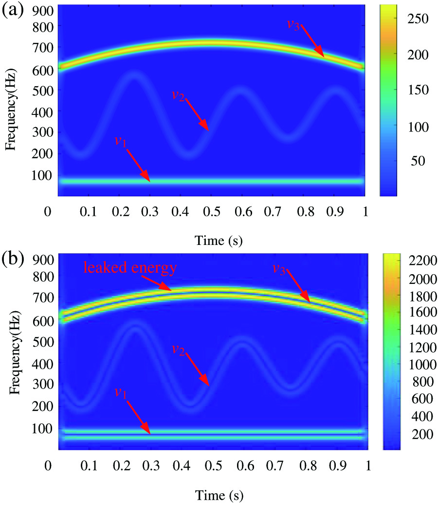Fig. 10. Analyzing results for the second significant point: (a) TFR obtained using STFT and (b) TFR obtained using OSTFT.

V.CONCLUSION

In this paper, we presented a novel TF analysis method called OSTFT by replacing the even symmetric window function with odd symmetric window function. Therefore, OSTFT can obtain a TFR with high TF resolution by acquiring minimum of 0 at time and frequency centers in the TF plane. It is worth to mention that the OSTFT can vitiate the effect of window size that we choose on the TFR obtained. Furthermore, the OSTFT has a satisfying performance on signals with complex IFs, even crossing IFs. The OSTFT has been validated by two numerical signals with complex IFs and two signals collected from a brown bat and from wind turbine vibration in the real life. The proposed OSTFT inevitably has its limitations. Because of the inherent property ignoring the amplitude information at time and frequency center, it is difficult for the OSTFT to reconstruct the signal.

Short-time Fourier Transform Using Odd Symmetric Window Function

I.INTRODUCTION

II.OSTFT

A.LIMITATION OF WINDOWED TRANSFORM

B.REVIEW OF STFT

C.PROPOSED OSTFT APPROACH

III.SIMULATION EVALUTION

A.CASE 1

B.CASE 2

IV.EXPERIMENT

A.EXPERIMENTAL CASE 1

B.EXPERIMENTAL CASE 2

C.DISCUSSION

V.CONCLUSION

References