I.INTRODUCTION
Remaining useful life (RUL) prediction, as the effective tool in reducing unplanned shutdowns caused by mechanical failures, is widely utilized in modernized industries to ensure the safety of machines and improve the production efficiency [1,2]. RUL prediction methods can mainly be divided into two categories [3], i.e., model-based methods and data-driven methods. Model-based methods aim to establish mathematical models to describe the machines degradation process through analyzing the physical failure mechanism. However, in practical cases, failure mechanism-based degradation model is generally difficult to formulate, and the mis-specification of degradation model will seriously impact the accuracy of RUL prediction. Compared with model-based methods, data-driven methods can adaptively model the degradation process without clear physical failure mechanisms through the utilization of machine learning (ML) technologies, such as support vector machine [4], gaussian process regression [5], artificial neural networks [6], etc. Therefore, data-driven methods have gained increasing attention in recent years.
Nevertheless, the above-mentioned data-driven methods merely use traditional ML methods, which results in limited prediction accuracy. Compared with traditional ML methods, deep learning (DL) methods have more powerful learning capabilities and possess the capability of establishing more complex mapping relationships [7] between monitoring data and RUL. Therefore, DL is now widely used in the field of RUL prediction [8–10]. Among various DL technologies, recurrent neural network (RNN) [11,12] and its variant, e.g., long short-term memory (LSTM) network [13–15], are able to effectively capture the time dependence hidden in the degradation process and have become the promising tool in RUL prediction. Although the existing approaches have demonstrated their RUL prediction effectiveness, they still suffering the following two limitations:
- 1)Since RNN lacks consideration of spatial correlation [16], it is difficult for RNN to extract directly degradation features from original monitoring data. Therefore, most of the RNN-based prognostic approaches are combined with hand-crafted features, which affect the accuracy and generalization of the forecast results, resulting in the fact that they are accurate only in some specific scenarios.
- 2)The uncertainty quantification of prognostic result is pivotal in making maintenance decisions, but most of the RNN-based RUL prediction methods only provide a point estimation. In the case of complex working conditions, the stability of RUL prediction results is often compromised, which would reduce the credibility of the method in providing guidance for predictive maintenance scheduling. Furthermore, the existing DL-based uncertain quantification methods mainly include two types: bootstrap [17] and Monte Carlo dropout [18] (MC dropout). Recently, Jason et al. [19] and Liu et al. [20] quantified the uncertainty of predicted RUL with bootstrap method. However, bootstrap-based methods require resampling the original training data and is time-consuming. Peng et al. [21] and Wang et al. [22] combined MC dropout with different neural networks to estimate the uncertainty. But MC-dropout-based methods need to run multiple times during the test stage, which is not efficient enough and requires additional computational burden.
To address the above-mentioned limitations, this paper proposes a new prognostic method named residual convolution long short-term memory (RC-LSTM) network for the RUL predictions of machines. In the proposed method, a ResNet-based convolution long short-term memory (Res-ConvLSTM) layer, which is improved from convolution long short-term memory (ConvLSTM) network [16], is first built to extract directly degradation representations and capture time dependence information from monitoring data. Then, an ordinary ConvLSTM layer is used to extract further degradation information. After that, predicated on the RUL following a normal distribution, an appropriate output layer is constructed to directly quantify the uncertainty of the forecast result without additional computational burden. Finally, the superiority of the proposed Res-ConvLSTM is validated using vibration data from accelerated degradation tests of rolling element bearings.
II.THE PROPOSED METHOD
The framework of RC-LSTM network is shown in Fig. 1. First, Res-ConvLSTM layer and ConvLSTM layer are stacked with batch normalization (BN) layer [23] to extract informative degradation representations. Then, the representations are input into normal distribution output layer to obtain the predicted RUL and to quantify uncertainty.
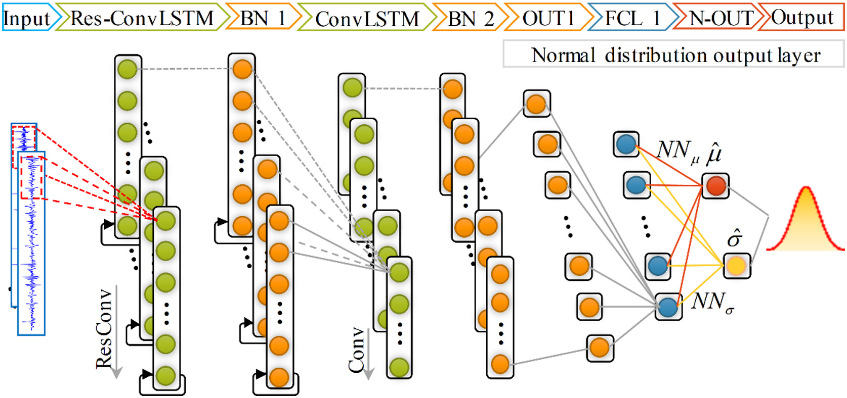 Fig. 1. Architecture of the proposed RC-LSTM.
In this section, we first introduce the ConvLSTM unit. Then, Res-ConvLSTM, where a new core building unit, improved from ConvLSTM, is further detailed. Finally, the normal distribution output layer and its loss function are described in details.
A.ConvLSTM UNIT
It has been justified that LSTM lacks consideration of spatial correlation, while in the meantime, CNN owns the capability of extracting spatial features. Accordingly, it is considered to embed CNN into LSTM to construct ConvLSTM unit to capture time series information and extract degradation representations simultaneously. The structure of ConvLSTM is shown in Fig. 2.
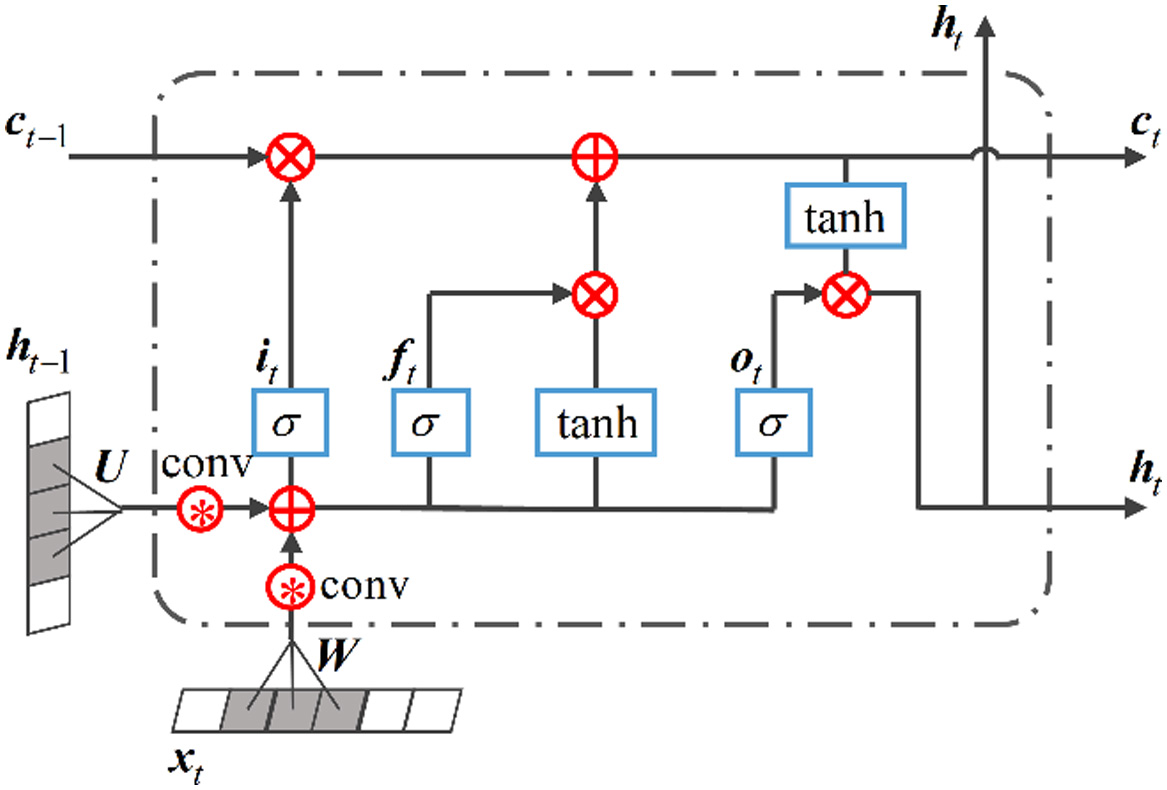 Fig. 2. The structure of ConvLSTM unit.
Given the current input , the hidden state and the cell state at previous moment, the output representation can be calculated as follows:
where , , and are input gate, forget gate, and output gate respectively. represents the convolution operator, is the current input, is the current cell state, and and are convolution kernels of different gates.Compared with the traditionally used LSTM, the main difference of ConvLSTM is that the fully connected structure in LSTM is replaced with the convolutional structure, which comprehensively utilizes the advantages of LSTM and CNN to extract simultaneously the local degradation feature and time dependence.
B.RES-ConvLSTM UNIT
As shown in Fig. 2, ConvLSTM uses single-layer convolution to extract local features from the current input . However, for complex original monitoring data, single-layer convolution is not sufficient to extract sensitive degradation representations. To address the above-mentioned problem, this paper constructs a Res-ConvLSTM unit, which utilizes deep residual convolutional neural network (Resnet) to replace single-layer convolution. The structure of Res-ConvLSTM unit is shown in Fig. 3.
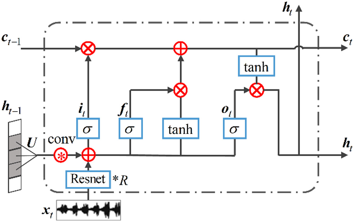 Fig. 3. The structure of Res-ConvLSTM unit.
Compared to ordinary convolutional neural networks, Resnet utilizes an identity mapping to address the problem of vanishing gradient and gradient explosion, which ensures the stability of network training when increasing the depth of network. Moreover, the structure of basic Resnet unit is shown in Fig. 4.
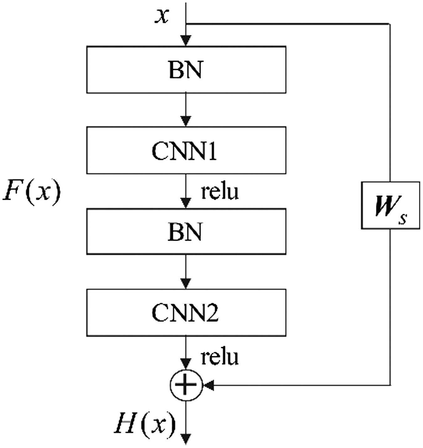 Fig. 4. The structure of basic Resnet unit.
Given the input vector , The output of Resnet unit is calculated as follows:
where is the output that ignores the identity mapping, and is a linear projection weight matrix, which aims to maintain the uniform dimensions of and .
Hence, by stacking R Resnet units to substitute the single-layer convolution, Res-ConvLSTM unit has greatly improved its local feature extraction capabilities, thereby realizing effective processing of massive monitoring data.
C.NORMAL DISTRIBUTION OUTPUT LAYER
Different from the traditional point estimation-based methods, this paper assumes that the predicted RUL follows a normal distribution and correspondingly constructs the normal distribution output layer to quantify uncertainty. The constructed layer is shown in Fig. 1, which exploits two different fully connected layers (FCLs), and , to obtain mean and standard deviation . Among them, the mean denotes the mean value of predicted RUL, and the standard deviation represents the uncertainty of the predicted result. Based on the above results, the conditional probability of RUL is obtained as:
where is the actual RUL and is the input of normal distribution output layer. Consequently, according to the mean and standard deviation , the prediction confidence interval (PI) corresponding to can be obtained as follows:Furthermore, since the standard deviation is an unknown prior, the supervised learning method is incapable of adjusting the parameters in . In view of this, the maximum likelihood estimation method is utilized to optimize the network parameters. Correspondingly, the log-likelihood loss function (LLF) is formulated as:
where n is batch size. During the training process, the goal is to find the optimal and that corresponds to the ascent direction of actual RUL condition probability. However, it is difficult to optimize simultaneously both mean and standard deviation for . Moreover, in some cases when actual RUL is known, another feasible option is to utilize mean square error (MSE) to optimize to ensure the accuracy of the predicted mean, then LLF can be further optimized with respect to both and . The loss function of the above-described optimization process is defined as:where and are the weights corresponding to MSE and LLF, which are adjusted with the training epoch.In addition, it is a commonsense that the more light-tailed the distribution of PI is, the more effective the maintenance scheduling can be. Based on this premise, the prediction interval averaged width [24] (PIAW) indicator is introduced into loss function to further clarify the optimization direction of standard deviation , The loss function is correspondingly defined as follows:
where and are the upper and lower limits of PI, respectively, and , , and are the weights corresponding to MSE, LLF, and PIAW, respectively.III.CASE STUDY: RUL PREDICTION OF ROLLING ELEMENT BEARINGS
To verify the effectiveness of the proposed RC-LSTM, vibration data collected from accelerated degradation tests of rolling element bearings are used, and four state-of-the-art prognostic approaches are compared in this section.
A.DATA DESCRIPTION
The datasets used in this paper are the XJTU-SY Bearing Datasets [3]. And the accelerated degradation tests of rolling element bearings are conducted in the testbed as shown in Fig. 5, which consists of an alternating current (AC) motor, a rotating shaft, a support bearing, a test bearing, a hydraulic loading system, a motor speed controller, etc. By controlling the speed and load, the testbed is capable of conducting degradation tests of bearings under different operating conditions.
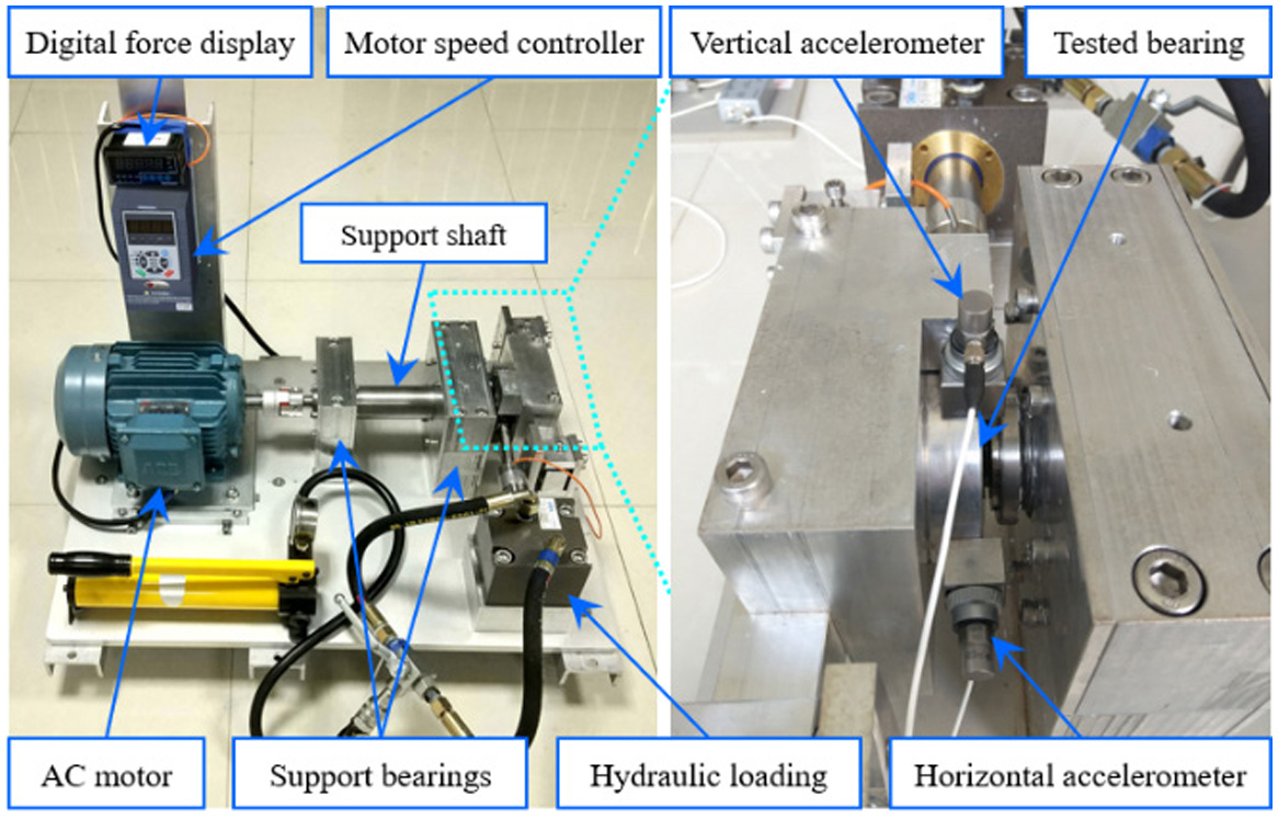 Fig. 5. Testbed of rolling element bearings.
As recorded in Table I, 15 LDK UER204 bearings were tested under 3 different operating conditions. During each test, two PCB 352C33 acceleration sensors were mounted in the horizontal and vertical directions of the test bearing to monitor the degradation process of the rolling bearing. And during the experiments, the sampling frequency was set to be 25·6 kHz, with the sampling time of 1·28 s and the sampling interval of 60 s. Put otherwise, 32768 data points can be obtained per sampling. In this section, Bearing1_4, Bearing2_4, Bearing3_4, Bearing1_5, Bearing2_5, and Bearing3_5 are selected as the testing dataset, respectively. And the remaining bearings are assigned as the training dataset.
| Radial force | Rotating speed/rpm | Bearing datasets |
|---|---|---|
| 12 kN | 2100 rpm | Bearing1_1 Bearing1_2 Bearing1_3 |
| 11 kN | 2250 rpm | Bearing2_1 Bearing2_2 Bearing2_3 |
| 10 kN | 2400 rpm | Bearing3_1 Bearing3_2 Bearing3_3 |
B.PROGNOSTIC METRICS
In this part, apart from the two commonly used prognostic metrics, RMSE and score function [25], two other metrics, i.e., accuracy [26] () and average interval score [27] (AIS), are also utilized to evaluate quantitatively the prediction performance. is a binary metric that evaluates whether the prediction result falls within at time . In this paper, and are set to 0·3 and 0·5, respectively. The AIS is employed to evaluate the comprehensive performance of the prediction interval, which is defined as follows:
where is the confidence level, is the interval length of the i-th PI, and S is the corresponding interval score that will impose punishment if the actual RUL is outside the PI. According to this definition, AIS is always a negative value that shares the positive correlation along with change of the convergence rate.C.CONFIGURATION OF RC-LSTM
Firstly, time window embedding is conducted on the monitoring data. Then, in RC-LSTM, the hyperparameters determined by grid search are summarized in Table II, and Adam optimizer is adopted to minimize the loss function. In addition, the weights in different loss functions are shown in Table III.
Table II. Configuration of RC-LSTM
| Hyperparameter | Size | Hyperparameter | Size |
|---|---|---|---|
| Number of Resnet units | 9 | Number of neurons in and | 100 |
| Number of kernels in Res-ConvLSTM | 256 | Number of kernels in ConvLSTM | 256 |
| Kernels size in Res-ConvLSTM | 3 × 1 | Kernels size in ConvLSTM | 3 × 1 |
| Time step | 7 | epoch | 100 |
| Batch size | 64 | Learning rate | 0·001 |
Table III. Weights in different loss functions
| Epoch | L2 | L3 |
|---|---|---|
| [0, 30] | ||
| (30, 60] | ||
| (60, 80] | ||
| (80, 100] |
D.RUL PREDICTION FOR BEARINGS
In this section, the advantages from the proposed loss function are first investigated and discussed. Then, the proposed RC-LSTM is compared with other state-of-the-art prognostics methods to demonstrate its superiority.
1)DISCUSSION OF LOSS FUNCTION
In addition to the ordinary LLF defined in, this paper proposes two different loss functions, i.e., defined in and defined in. To illustrate the advantages of and , all three loss functions are used to predict the RUL of bearings. Fig. 6 shows the prediction results of Bearing 3_5 under different loss functions. Meanwhile, the performance estimation results under all three scenarios are tabulated in Table IV where the bolded values are the best evaluation results.
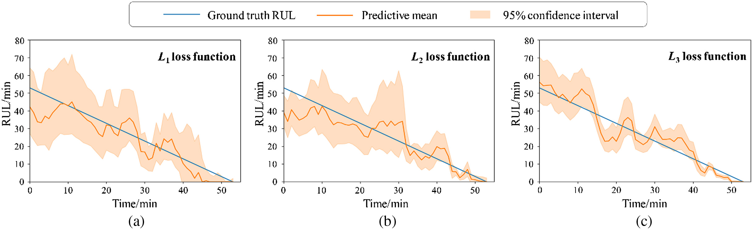 Fig. 6. RUL prediction results of Bearing3_5 under different loss functions. (a) L1 loss function. (b) L2 loss function. (c) L3 loss function.
Table IV. The performance estimation results of these three loss functions
| Metrics | L1 | L2 | L3 | |
|---|---|---|---|---|
| Bearing 1_5 | RMSE | 8.04 | 5.91 | |
| Score | 22.28 | 18.73 | ||
| AIS | −23.21 | −21.83 | − | |
| 53.48% | 69.44% | |||
| Bearing 2_5 | RMSE | 30.21 | 29.40 | |
| Score | 3358.18 | 3165.99 | ||
| AIS | −131.65 | −123.88 | − | |
| 52.69% | 53.30% | |||
| Bearing 3_5 | RMSE | 5.85 | 5.35 | |
| Score | 32.53 | 25.24 | ||
| AIS | −35.97 | −33.42 | − | |
| 59.26% | 64.81% | |||
It can be observed from Table IV and Fig. 6 that in the RUL prediction of bearings, compared with ordinary LLF L1, both L2 and L3 achieve lower RMSE score values and higher values, which indicates that by introducing MSE and prioritizing the optimization of prediction mean , the performance of network can be effectively improved, and the mean value of RUL prediction results can be obtained with higher accuracy. Moreover, it can also be clearly seen that by considering the directional optimization of prediction standard deviation , the PI corresponding to L3 is significantly narrower than that of L1 and L2, which means L3 is able to reduce sufficiently the uncertainty of prediction results and provide a more applicable PI. As a result, benefiting from introducing the MSE and PIAW, the proposed loss function effectively improves the performance of prognostics model.
2)COMPARISON WITH THE STATE-OF-THE-ART PROGNOSTICS METHODS
In this section, three other state-of-the-art point estimation prognostics approaches are firstly implemented to predict RUL for bearings for comparison, which are named as N1, N2, and N3, respectively. Among them, N1 [28] first converts the time domain signal into the frequency domain, then inputs it into one-dimensional CNN and simple recurrent unit network to realize RUL prediction. N2 [29] utilizes LSTM and attention mechanism to learn degradation representations from original monitoring data and predict RUL. N3 [30] is a prognostics method that combines CNN, LSTM, and attention mechanism. Table V summarizes the evaluation metrics of different networks.
Table V. The performance estimation results of different networks
| Bearing dataset | N1 | N2 | N3 | Proposed | ||||
|---|---|---|---|---|---|---|---|---|
| RMSE | Score | RMSE | Score | RMSE | Score | RMSE | Score | |
| Bearing1_4 | 9.76 | 100.84 | 9.35 | 89.79 | 9.21 | 82.91 | ||
| Bearing2_4 | 14.67 | 218.11 | 17.89 | 363.04 | 15.41 | 285.24 | ||
| Bearing3_4 | 36.66 | 6151.82 | 44.75 | 7576.17 | 37.57 | 6503.24 | ||
| Bearing1_5 | 5.98 | 18.70 | 6.52 | 20.77 | 6.04 | 17.64 | ||
| Bearing2_5 | 31.31 | 4036.24 | 32.89 | 2158.24 | 27.39 | 2467.59 | ||
| Bearing3_5 | 5.85 | 32.10 | 6.48 | 37.56 | 5.23 | 25.17 | ||
The result shows that the proposed RC-LSTM gets the lowest RMSE values in all cases and the lowest score values in all cases but one. This signifies the superiority of RC-LSTM, compared to the three state-of-the art methods in RUL prediction accuracy. More importantly, RC-LSTM is capable of providing a probabilistic distribution to quantify uncertainty, which overcomes the limitation of traditional point estimation prognostics approaches. Therefore, the prediction performance of RC-LSTM is more useful in applications than the other three methods.
To further verify the performance of the proposed method, we also compare the proposed method with other DL-based uncertainty quantification methods, including Bayesian multiscale CNN-based method [21] (BMSCNN) and Bayesian recurrent convolutional neural network [22] (BRCNN). Among them, BMSCNN combine Monte Carlo dropout with deep multiscale CNN to achieve uncertainty quantification. BRCNN first constructs a network structure named recurrent convolutional neural network and then utilizes MC dropout to quantify the uncertainty. The comparison results are tabulated in Table VI.
Table VI. The performance estimation results of different DL-based uncertainty quantification methods
| Bearing dataset | BMSCNN | BRCNN | Proposed | |||||||||
|---|---|---|---|---|---|---|---|---|---|---|---|---|
| RMSE | Score | AIS | RMSE | Score | AIS | RMSE | Score | AIS | ||||
| Bearing1_4 | 11.66 | 84.39 | 43.33 | −153.39 | 9.68 | 92.24 | 56.67 | −83.90 | − | |||
| Bearing2_4 | 18.81 | 450.61 | 42.50 | −191.00 | 13.41 | 55.00 | −87.54 | 184.15 | − | |||
| Bearing3_4 | 46.41 | 7437.45 | 31.85 | −345.36 | 40.60 | 6518.99 | 39.49 | −273.61 | − | |||
| Bearing1_5 | 9.15 | 30.76 | 47.83 | −31.38 | 6.28 | 21.82 | 66.09 | −29.99 | − | |||
| Bearing2_5 | 27.30 | 4767.90 | 46.71 | −141.27 | 24.06 | 2204.14 | 58.68 | −127.24 | − | |||
| Bearing3_5 | 6.59 | 35.68 | 55.56 | −37.00 | 5.54 | 26.98 | 64.81 | −34.01 | − | |||
From this table, it can be clearly seen that the proposed method gets lower score RMSE values and higher values, which indicates the proposed RC-LSTM achieves higher prediction accuracy than BMSCNN and BRCNN. Furthermore, the AIS value of the proposed method is significantly higher than other uncertainty quantification methods, and this means that the proposed RC-LSTM achieves a better trade-off between the prediction interval coverage and the interval width. Based on the above analyses, the RC-LSTM has a slightly better performance than other DL-based uncertainty quantification methods in RUL prediction of bearings.
IV.CONCLUSION
This paper proposed a new prognostics method named RC-LSTM to predict machine RUL. In the RC-LSTM, a residual convolution long short-term memory layer was constructed to extract degradation representations from monitoring data. Then, a ConvLSTM layer was stacked to capture subsequent time dependence. After that, through constructing a normal distribution output layer and an improved loss function, the proposed method could effectively quantify the uncertainty of prediction results. Finally, bearing vibration data were employed to evaluate the proposed RC-LSTM, and prediction results were compared with some state-of-the-art prognostics methods. Experimental results indicated the effectiveness and superiority of the proposed method. Moreover, different from traditional point estimation based prognostics approaches, the RC-LSTM can provide probabilistic prediction results, which facilitates making maintenance decisions effective.