I.INTRODUCTION
Dry friction plays an important role in both daily life and engineering. It exists between two contacting surfaces [1,2]. Dry friction can transfer kinetic energy to thermal energy and thus dissipates the energy of a friction system. However, a friction system will vibrate when the input energy is higher than the dissipated energy, and such vibration is called friction-induced stick-slip vibration (FIV) [3,4]. Stick-slip vibration is a kind of FIV and is non-smooth with strong nonlinear properties [5,6]. It contains two kinds of motion: stick motion when the relative speed between two frictional contact surfaces is zero; slip motion when the relative speed is non-zero [7,8].
Stick-slip vibration is very common in nature. In some cases, it is useful, as in string instruments [9,10], or as the friction damper [11]. In other cases, it has to be reduced or suppressed because it can induce noise [12]. The stick-slip vibration of earth plate may case devastating earthquake [13]. Therefore, it is very important to understand and control stick-slip vibration.
Stick-slip vibration has attracted many researchers [14–20]. Popp and Stelter [14] studied bifurcation and chaotic behavior of two discrete and continuous models of stick-slip systems. Wei et al. [15] built a theoretical pad-on-disc model and used the Stribeck model to study nonlinear properties of the friction system, and the results showed that the friction system had Hopf double-bifurcation and chaos phenomenon as the reduction of angular velocity. Oberst and Lai [16] built a pad-on-disc finite element model and found that intermittently chaotic pad motion could excite disc quasi-periodic dynamics; the chaotic motion of the pad could produce a toroidal attractor of the disc’s out-of-plane motion. Massi et al. [17,18] studied the evolution process of steady sliding to macroscopic stick-slip vibration to unstable mode coupling. Wang et al. [19] built a two-degree-freedom model based on experimental study to investigate the characteristics of stick-slip vibration.
Stick-slip vibration seems very sensitive to work conditions, for example, the normal force, the relative velocity, and the contacting materials [21–24]. Leus et al. [21] performed an experimental study and found that tangential vibrations induced by a piezoelectric inductor helped reduce and even eliminate stick-slip vibration in their test structure. Dong et al. [22] discovered that the noise mainly occurred during the slip phase, and the relative speed and external load had a strong influence on main vibrational frequency. Yoon et al. [23] studied stick-slip vibration of a brake system and found that the normal load, disc velocity, and interface topography of the friction pair could influence whether the friction system exhibited stick-slip vibration.
The normal force of a real friction system is often time varying [25–29]. Pasternak et al. [26] investigated stick-slip vibration properties using a one-degree-freedom model and found that the fluctuation of normal force could affect friction properties significantly. Numerical work by Krallis et al. [28] revealed that a harmonic normal force could suppress the stick-slip vibration. Wang et al. [29] found that the normal force showed various degrees of fluctuation with different contacting materials. Actually, studies of the effect of the time-varying normal force on stick-slip vibration are limited. The lack of research into stick-slip vibration under a time-varying normal force is the motivation of this paper.
In this paper, comparative experiments are conducted with a constant normal force of different fixed magnitudes and a harmonic normal force with various frequencies, respectively. Then mathematical tools, such as phase space reconstruction, are used to reveal the science behind the complicated dynamic behavior. In section 2, the test rig, experimental parameters, and mathematical tools are introduced. In section 3, the experimental results under different kinds of normal force are presented. In section 4, the phase space reconstruction analysis is performed to show the intrinsic dynamics of FIV under different normal force. The conclusions are presented in section 5.
II.EXPERIMENTAL SETUP AND ANALYSIS METHOD
A.EXPERIMENTAL SETUP AND PARAMETERS
In this work, the experiments are performed on a pad-on-disc configuration installed on a UMT-3 CETR tribometer. Its schematic can be seen in Fig. 1, and the details and operational process of the setup can be found in reference [29]. This setup has the advantage of a well-defined contact area and a simple friction pair, which creates a rather simple structure and thus helps understanding of the characteristic of stick-slip phenomena under different working conditions. A laser vibrometer (No.: Polytec PDV-100; sensitivity: 100 mV/mm/s; frequency range: 0·5–22 kHz; measuring range: ±50 mm/s) is used to record the tangential velocity of pad during the tests. A triaxial accelerometer (brand: KISTLER 8688A50; sensitivity: 100 mV/g; frequency range: 0·5–5 kHz; measuring range: 50 g) is used to record the normal, tangential, and radial acceleration. An 8-tunnel acquisition and analysis system (No.: DH5922N) is used to collect and analyze signals during the experiments, and the sample frequency is set to be 10 kHz.
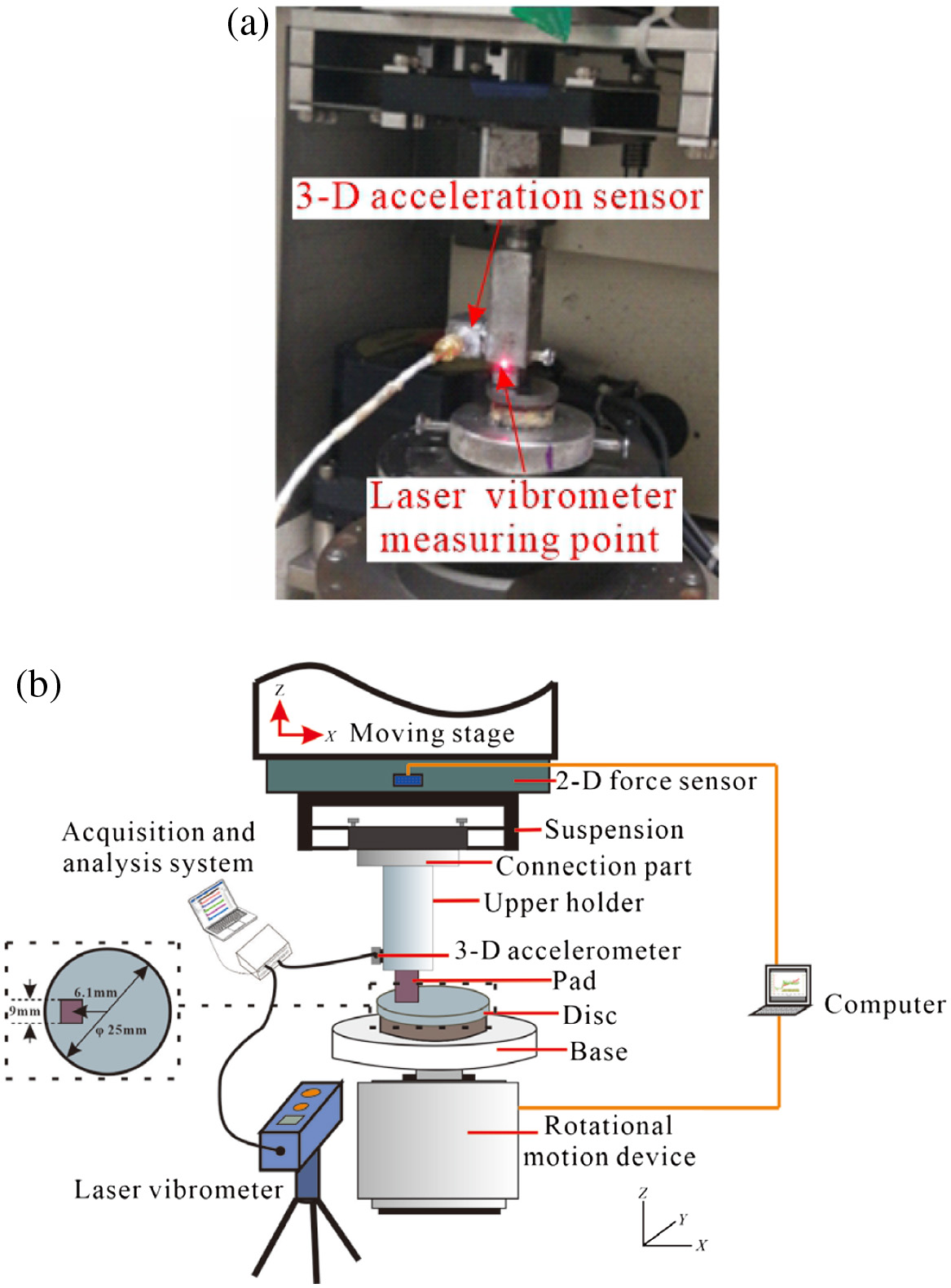 Fig. 1. Photo (a) and schematic diagram of the test setup (b).
The pad is made from composite material of a real brake pad whose thickness is 15 mm and contact interface is 9×9 mm2. Its main material properties are density is 1 ± 0·5 g/cm3; Young’s modulus is E≤1×10³ MPa; hardness is HR 50–90; and interface roughness (Ra) is approximately 0·4 μm which is measured by a profilometer before the tests. The disc is made from forged steel, and its diameter is 25 mm and thickness is 3 mm. The disc is first polished with silicon carbide abrasive paper and then polished with cloth until they achieve the initial average roughness (Ra) (measured by a profilometer) of the surfaces approximately at 0·06 μm.
In this work, the normal force is described by
where F0 is the constant part (mean value) of the normal force, A is its oscillation amplitude, ω is its oscillation frequency, and t is time. F0 and ω will be different in different tests. In this work, a series of pre-tests are performed to examine which parameters can excite visible stick-slip vibration (without severely irregular vibration behavior), under the hardware constraint of the tribometer.For the constant normal force, A and ω are set to be 0 and F0 is set to 160 N, 180 N, and 200 N, respectively, to investigate the influence of magnitude of the normal force on stick-slip vibration. For the harmonic normal force, F0 is set to be 180 N, A is set to be 20 N, and ω is set to be 0·25 Hz, 0·5 Hz, 1 Hz, and 2 Hz (the oscillation frequency selection is limited to 2 Hz due to the hardware restriction of the tribometer), respectively, to study the effect of the oscillation frequency of the normal force on stick-slip vibration. The various cases of the applied normal force used in the tests are summarized in Table I. To make the paper more readable, the various cases are named with “short names,” as shown in Table I.
Table I. Parameters of normal force
| Mean value (N) | Amplitude (N) | Frequency (Hz) | Short name |
|---|---|---|---|
| 160 | 0 | / | Case 1 |
| 180 | 0 | / | Case 2 |
| 200 | 0 | / | Case 3 |
| 180 | 20 | 0·25 | Case I |
| 180 | 20 | 0·5 | Case II |
| 180 | 20 | 1 | Case III |
| 180 | 20 | 2 | Case IV |
During the tests, the velocity of disc is set to be 2·5 rpm and the friction radius is 6·1 mm, which means a linear velocity of 1·597 mm/s. Each test lasts 2 minutes, and at least three repeated tests are performed under each kind of working condition to ensure good repeatability. At first, a desired normal force is applied and then the disc starts to rotate after the normal force achieves the set value. All the tests are conducted under the same atmospheric conditions with strictly controlled relative humidity of 60% ± 10% and ambient temperature of around 25°C.
B.PHASE SPACE RECONSTRUCTION OF TIME SERIES
FIV has strong nonlinearity, which cannot be well handled by the traditional time series analysis method for its limitations to reveal the evolutional regularity and characteristics of the stick-slip vibration. Therefore, a phase space reconstruction method is used to transform the signals from one dimension to high dimension to reveal its dynamic properties, such as the chaotic attractors of a friction system [30,31]. In this work, the method of parameter selection of the phase space reconstruction of time series analysis followed mainly reference [30].
1)DETERMINATION OF RECONSTRUCTION EMBEDDING DIMENSION AND DELAY TIME
The phase space reconstruction method is a key technique for nonlinear time series analysis. A suitable embedded dimension m and time delay τ are two very important parameters for this method.
An original time series can be rearranged into the following matrix in Eq. (2):
where M = N−(m−1)τ is the number of phase points in phase space.A C-C method [32] which combines the advantage of the autocorrelation function and auto-mutual information function, is applied in this work, which can determine the optimal values of m and τ simultaneously [32] by increasing m and decreasing τ while keeping embedded window width τω in Eq. (3) as a constant
For a time series x(i) i=1,2,3,…N, with length N, it can be divided into n disjoint time sub-series with length [N/n] ([] is rounding function), as shown in Eq. (4). The statistical magnitude S(m,N,d,τ) of every time sub-series can be expressed in Eq. (5), where Cl is the correlation integral of the l-th time sub-series shown in Eq. (6), in which θ(·) is the Heaviside unit function and d is the radius of neighborhood.
when N→∞,Based on the Brock-Dechert-Scheinkman (BDS) statics, if the time series is independent and identically distributed, S(m,d,τ) approaches 0 when N→∞. S(m,d,τ)∼τ can well reflect the autocorrelation characteristics of the time series. When S(m,d,τ) passes through the zero point or the differences are minimal for all of d, the points representing the time sub-series in the reconstructed phase space are almost uniformly distributed and the reconstructed attractor trajectory is completely expanded in the phase space.
ΔS(m,τ) (as shown in Eq. (8)–(11)) is defined to measure the maximum deviation of S(m,d,τ)∼τ from all of d. According to the numerical results, the first zero point of S(m,d,τ)∼τ or the first minimum of ΔS∼τ is selected to be the optimal delay time τ in this work.
The parameters of N, m, and d can be reasonably estimated by applying the BDS. In this work, the parameters are set to be: N = 3000; m = 2, 3, 4, 5; dk = kσ/2, k = 1, 2, 3, 4, where σ is the standard deviation of the time series.
In the current C-C method, the first zero point of or the first minimum point of is the optimal τ and the global minimum point of Scor(n) is the τω. Based on the theoretical description above, the optimum embedded dimension m and time delay τ of phase space reconstruction can be obtained in MATLAB.
2)PRINCIPAL COMPONENT ANALYSIS
The phase space reconstruction is applied on time series to transform it from one-dimensional vector to m-dimensional spatial vector. The principal component analysis (PCA) reduces the reconstructed m-dimensional vector to d-dimensional linearly unrelated vectors by dimensionality reduction. In this work, d is set as 3 to allow for a visual representation of the reconstructed attractor. The correlation coefficient matrix is obtained through MATLAB function corrcoef, and the eigenvalues and eigenvectors of the matrix are calculated and sorted. The eigenvectors of larger eigenvalues make higher contributions to whole time series, which are called the principal components. Usually, the first three principal components are sufficient.
3)RECURRENCE PLOT
Recurrence plot (RP) can be used to analyze the periodicity, chaos, and non-stationarity of a time series. The pattern of phase space trajectory evolution with time can be explored from the overall structural characteristics of the plot. With the obtained m, τ, and the original time series data as inputs, the RP of the system can be obtained using the MATLAB Toolbox CRPtool [33].
III.EXPERIMENTAL RESULTS
A.VIBRATION UNDER CONSTANT NORMAL FORCES
Figure 2 shows the friction force of the experimental system and the relative velocity (the difference between the pad tangential velocity and the disc velocity) between the pad and the disc in steady-state stage (50–52 s). It can be found that the friction force shows a regular sawtooth pattern, and the vibration is a stick-slip type from Fig. 2(a). The friction force increases slowly at the stick stage before it reaches the break-away force, then it jumps down to the dynamic friction force immediately afterwards [29], and the relative motion between the pad and the disc changes from stick to slip. Furthermore, with the increasing magnitude of the constant normal force, the break-away force and the dynamic friction force become higher, and the difference between break-away forces also becomes higher.
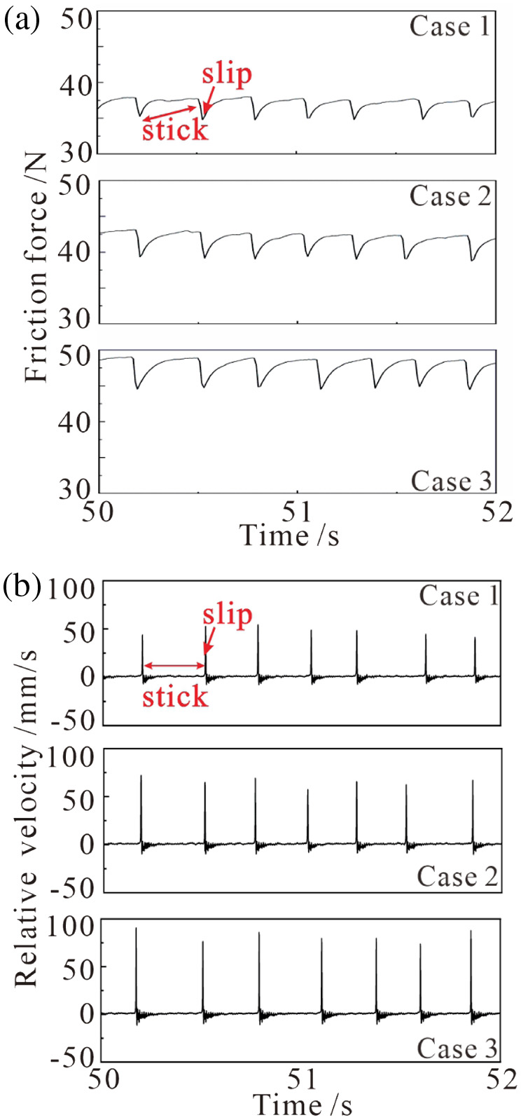 Fig. 2. Friction force (a) and relative velocity (b) under constant normal force.
Figure 2(b) shows the relative velocity in time domain, which is the difference between the disc velocity and the pad velocity. Stick-slip vibration is apparent. A higher constant normal force leads to a bigger relative velocity jump at stick to slip transition, which is consistent with the previous findings [19].
Since the experimental results and RPs under each constant normal force show similar trends, only the phase plane for Case 2 is shown in this work, as given in Fig. 3. The displacement is calculated numerically using MATLAB. Obviously, the displacement-velocity phase plane forms limit cycles.
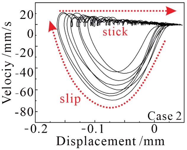 Fig. 3. The velocity-displacement phase plane of the friction system under constant normal force.
Two motion regimes can be found in the limit cycles: stick motion and slip motion as shown in Fig. 3. During the stick stage, the velocity of pad almost keeps the same with the disc with slight oscillation, this is because of the inevitable slight oscillation of the test rig. The displacement of pad and stored tangential elastic potential energy of the friction system increase with pad motion during the stick stage, the elastic potential energy reaches the maximum when the displacement is the maximum. After this moment, the elastic potential energy is released to be kinetic energy and the pad starts to slid on disc, the velocity increases from zero, the relative motion changes from stick motion to slip motion.
Figure 4 shows vibration acceleration of the pad measured by the accelerometer in the tangential direction during a whole test, under constant normal force of 180 N. It can be found that the acceleration shows periodic “Sudden Jump” [29] due to sudden switching from stick regime to slip regime. The jump magnitude increases with the normal force. In contrast, the acceleration is almost zero during the stick regime.
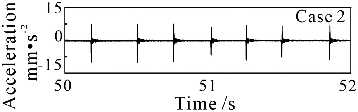 Fig. 4. Tangential acceleration under constant normal forces of 180 N.
The root mean square (RMS) values of the vibration accelerations under different normal force levels are also calculated. These are 0·544 m/s2, 0·768 m/s2, and 1·004 m/s2 for Case 1, Case 2, and Case 3, respectively. The results indicate that the friction system undergoes stronger vibration under a higher constant normal force.
To get a deep insight of the effect of a constant normal force on stick-slip vibration, Table II lists the statistics of the main parameters of stick-slip vibration. In Table II, μmax is the maximum friction ratio (ratio of friction force to normal force), μmin is the average of the minimum friction ratio, Δμ is the difference between μmax and μmin, and X is the tangential displacement of the pad. These very important parameters reflect the intensity of stick-slip vibration. It can be found that Δμ increases from 0·0177 to 0·0198, with the increase of constant normal force from 160 N to 200 N.
Table II. Statistics of main parameters of stick-slip vibration under constant normal force
| Cases | μmax | μmin | X (mm) | Δμ |
|---|---|---|---|---|
| Case 1 | 0·2355 | 0·2178 | 0·155 | 0·0177 |
| Case 2 | 0·2366 | 0·2187 | 0·168 | 0·0179 |
| Case 3 | 0·2436 | 0·2238 | 0·213 | 0·0198 |
The stick-slip vibration is also investigated in frequency domain using the fast Fourier transform (FFT), and the results are shown in Fig. 5. It can be found that there is not a main frequency, but the energy level increases with the higher constant normal force. Furthermore, it decreases as the frequency increases for each kind of constant normal force. The FFT results indicate that the higher constant normal force causes stronger stick-slip vibration.
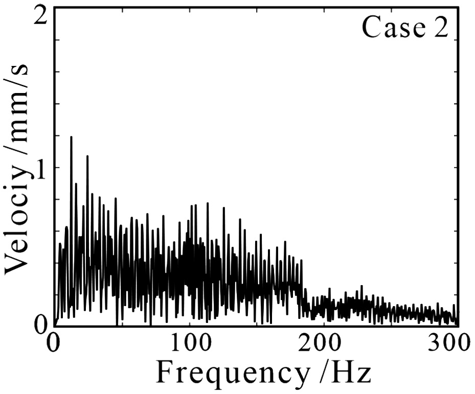 Fig. 5. FFT results of tangential velocity under constant normal force of 180 N.
B.VIBRATION UNDER HARMONIC NORMAL FORCES
In this part, the harmonic normal force with various oscillation frequency is applied, and the friction force and normal force in steady stage (50–55 s) are shown in Fig. 6. Obviously, the friction force and normal force share the same oscillation frequency, which is determined by the normal force. The friction force is very smooth when the harmonic normal force is increasing. In contrast, it exhibits visible oscillation when the normal force is decreasing, and its amplitude is smaller with higher oscillation frequency of the harmonic normal force.
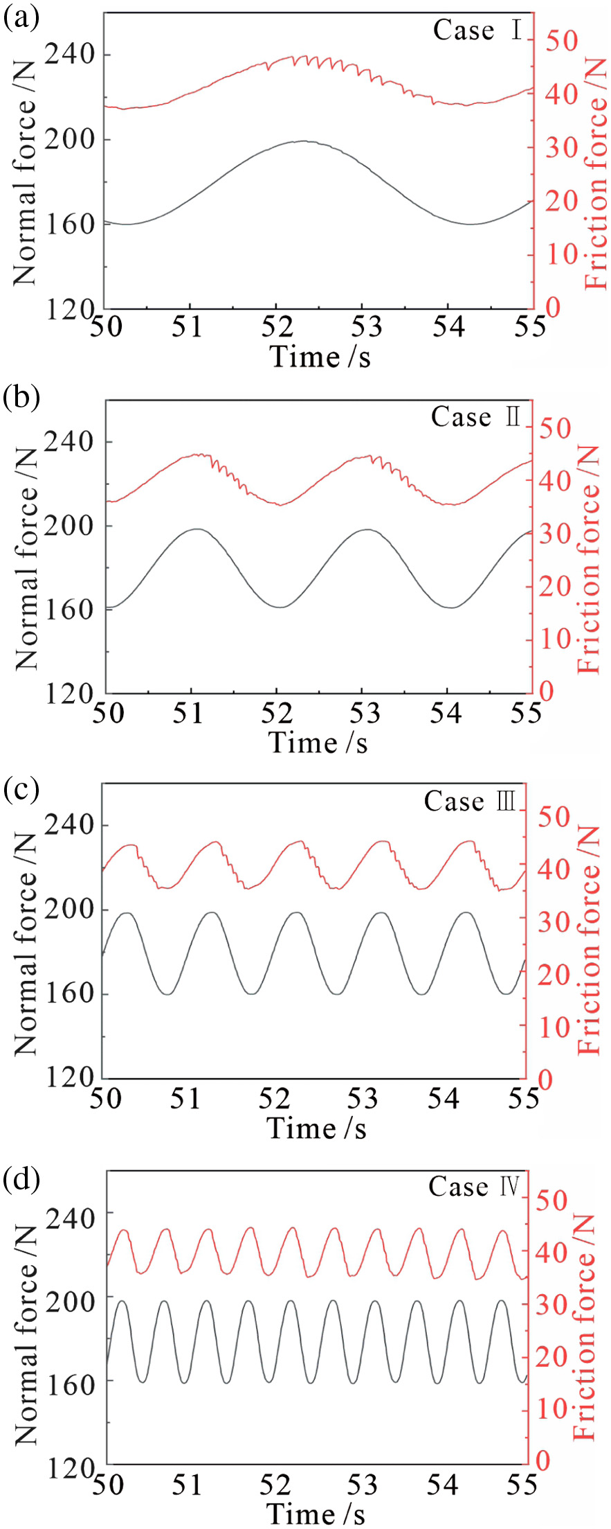 Fig. 6. Friction force and harmonic normal force in steady stage.
Figure 7 shows the relative velocity and the friction ratios under normal forces with various oscillation frequencies. They show fairly regular oscillation, similar to the friction force. They also share the same oscillation period as that of the normal force, which are T1 (4 s), T2 (2 s), T3 (1 s), and T4 (0·5 s) corresponding to Case I, Case II, Case III, and Case IV, respectively.
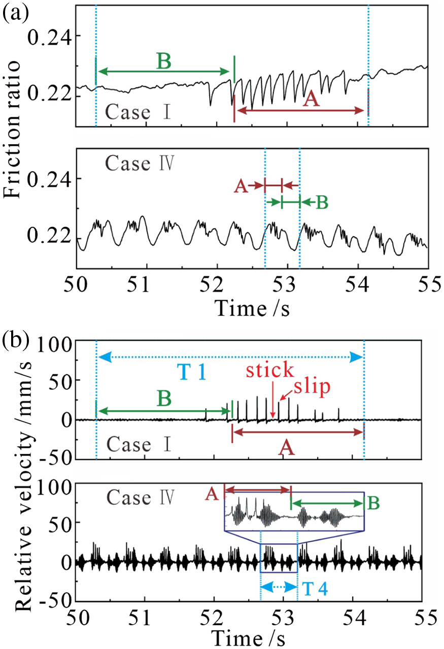 Fig. 7. Friction ratio (a) and relative velocity (b) in time domain under different harmonic normal force.
For clarity, two stages in relative velocity/friction ratio are defined in Fig. 7: A and B stages corresponding to the decreasing and increasing harmonic normal forces, respectively.
The friction system shows stick-slip vibration at A stage for Case I. Visible sudden jumps in the relative velocity and regular sawtooth in the friction ratio can be found at this stage, because the break-away force reduces with decreasing harmonic normal force in this stage, and the external tangential force is higher than the break-away force. For B stage, the relative velocity and the friction ratio are very smooth, no stick-slip vibration can be found, and the relative velocity is zero at this stage. Therefore, the relative motion between the pad and the disc is stick motion, because at B stage the break-away force increases with increasing harmonic normal force, the break-away force is always higher than the elastic restoring force in the tangential direction.
The relative velocity shows sudden jumps and high frequency oscillation at A stage for Case IV, but it only shows high frequency oscillation at B stage, and there is smooth motion between the pad and the disc. The friction ratio shows complicated multi-frequency oscillation.
The tangential acceleration of the pad and its RMS values are shown in Fig. 8. Nearly periodic sudden jumps are present for Case I, due to stick-slip vibration. The jump magnitude reduces with the oscillation frequency of the harmonic normal force. In addition, for these three kinds of harmonic normal forces, the RMS values of accelerations are relatively low, which are 0·220 m/s2, 0·214 m/s2, and 0·242 m/s2, corresponding to Case I, Case II, and Case III, respectively.
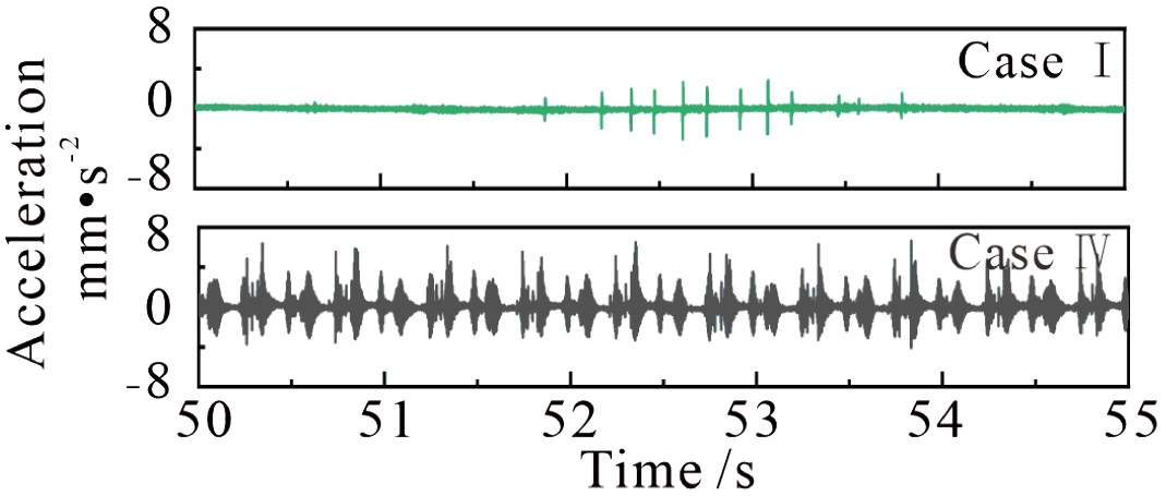 Fig. 8. Tangential vibration acceleration under various harmonic normal force.
The acceleration is significantly different from that for Case IV compared. There is an obvious increase in its magnitude and intermittent chaotic oscillations can also be seen, with stronger vibration (the RMS of acceleration is 1·026 m/s2).
Compared with the tangential acceleration of the pad under the constant normal force in Fig. 4, it can be found that the vibration of the friction system is reduced for Case I. Particularly, the stick-slip vibration is suppressed at the increasing stage of harmonic normal force. In contrast, the friction system shows stronger vibration for Case IV. It can be preliminarily concluded that the oscillation frequency of harmonic normal force has a significant effect on the vibration of the friction system: its intensity and vibration regime.
The phase plane of the pad is plotted in Fig. 9. Compared with the displacement-velocity phase plane in Fig. 3, the limit cycles are much smaller. Two kinds of distinguished motions can be found for Case I: stick and slip motion, which further conforms that stick-slip vibration is possible under harmonic normal forces.
 Fig. 9. The phase plane under harmonic normal forces.
In addition, there is effectively one limit cycle in the phase plane corresponding to the Case I. No clear limit cycle can be found in the phase plane for Case IV, and the cluttered trajectories suggest chaotic motion.
These phase-plane results show that the friction system undergoes nearly periodic stick-slip vibration under a constant normal force, but can exhibit a complicated periodic vibration under a harmonic normal force.
How system frequencies evolve with time can be revealed via a wavelet transform and such results are presented in Fig. 10.
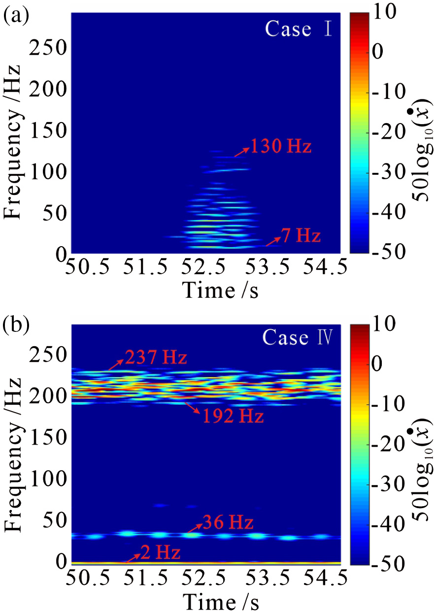 Fig. 10. Time-frequency signal under harmonic normal force.
In Fig. 10(a), a broadband frequency range of 7∼130 Hz is visible with several concentrated energy distribution occurring at 52·5∼53·5 s for Case I. This phenomenon is due to the stick-slip vibration in this time range (as shown in Figs. 7–9). There is no strong frequency component in the other time duration due to the absence of stick-slip vibration.
The frequency components in Fig. 10(b) are much complex compared with those of the other three cases. There is one main frequency at 34·4 Hz and one time-continuous narrow frequency band (in 192∼237 Hz) with higher energy than the former. The frequency of 2 Hz of the harmonic normal force can also be detected.
The frequency domain results show that the frequency of the harmonic normal force has a significant influence on the system vibration behavior; it can modify the main frequency of the system vibration. Stick-slip vibration is excited when the forcing frequency is relatively low (0·25 Hz in this work). A high forcing frequency (2 Hz in this work) tends to excite a high-frequency FIV in this work.
IV.PHASE SPACE RECONSTRUCTION ANALYSIS
The experimental results show that the oscillation frequency of harmonic normal force can modify not only the vibration intensity but also the distribution of vibration main frequency of friction system. Especially, the vibration mode of the friction system can even be modified when the oscillation frequency is high enough.
In this section, the nonlinear time series analysis is performed to study the dynamic property of the friction system with various normal force. Firstly, the C-C method is adopted to reconstruct the phase space of time series using the correlation integral to obtain the embedding dimension m and the optimal delay time τ. Then, the m-dimensional phase space vector is mapped in the three-dimensional visual phase space diagram through PCA. And map the RP through the RP algorithm using MATLAB CRPtool toolbox according to the determined τ and m.
In this work, the tested pad velocity is set as the input for phase space analysis. Compared with other signals as the inputs, the results of phase space reconstruction analysis with this kind of input can well display the dynamic characteristics of friction system under different normal force. Firstly, the velocity is normalized to the range of 0–1, and then the three-dimensional visual phase space diagram and RP are mapped with the determined τ and m.
A.PHASE SPACE RECONSTRUCTION ANALYSIS RESULTS CONSTANT NORMAL FORCE
Firstly, the phase space analysis is performed to study the dynamic property of friction system. Similar to Section 3·1, the phase space analysis results of Case 2 are presented. The velocity time series of 1 s is reconstructed and m = 6 and τ = 4 are obtained. The phase space analysis results are shown in Fig. 11. Firstly, the velocity is normalized to the range of 0–1, as shown in Fig. 11(a). Four cycles of stick-slip vibration can be found.
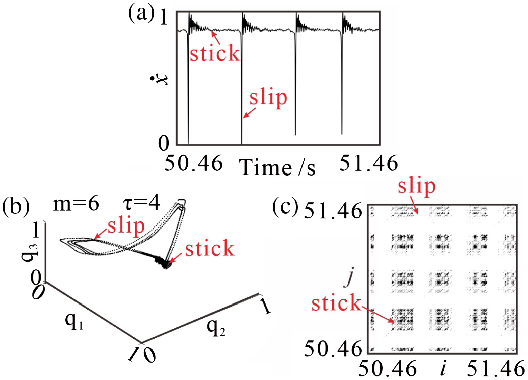 Fig. 11. Normalized velocity of pad (a), orbital diagram of velocity in the three-dimensional phase space (b) and RP of velocity (c) under constant normal force (Case 2).
The reconstructed velocity in the three-dimensional phase space is shown in Fig. 11(b). The reconstructed orbit at the slip stage spreads in the phase space, but the reconstructed orbit at the stick stage is localized and curled up into a small black area. It should be noted that the velocity should be the same constant value as the disc velocity, but the pad velocity shows some oscillation due to vibration of the test rig. Therefore, the reconstructed orbit at the stick stage is a small area instead of a single spot.
The RP of velocity is shown in Fig. 11(c). Large alternating white and black areas appears in the RP, due to sudden sharp motion state changes in the friction system, which indicates that the different cycles of stick-slip vibration share the same frequency. The black block area, corresponding to the stick stage, is uniformly composed of some isolated points, short diagonal lines (the whole RP is symmetric about the diagonal line, the diagonal lines in RP are parallel or coincident with the short diagonal line), and vertical lines, and indicates that the vibration of the friction system shows the uncertainty.
B.PHASE SPACE RECONSTRUCTION ANALYSIS RESULTS UNDER HARMONIC NORMAL FORCE
The experimental results in Fig. 7 show that the decreasing stage A and increasing stage B of harmonic normal force have very different effects on vibration behavior of the friction system. Therefore, the velocity time series is divided into different segments of the same length for phase space reconstruction analysis. The sampling frequency is set to be 10 kHz in the experimental study, and samples in at least 0·5 s are taken for the four kinds of harmonic normal force (as shown in Fig. 6); therefore, 5000 sampling points are used (2500 sampling points in A and B stages, respectively.) The phase space analysis results are shown in Figs. 12–16, with figures in red and green frames for A and B stages, respectively.
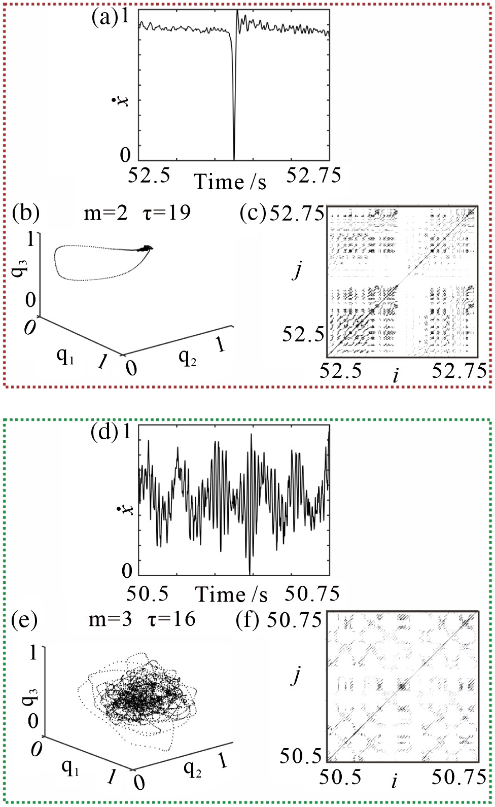 Fig. 12. Phase space reconstruction results of A and B stages of Case I.
 Fig. 13. Phase space reconstruction results of A and B stages of Case II.
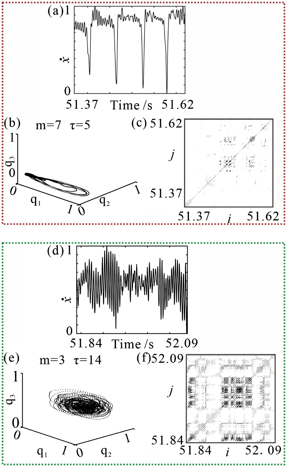 Fig. 14. Phase space reconstruction results of A and B stages of Case III.
 Fig. 15. Phase space reconstruction results of A stage of Case IV.
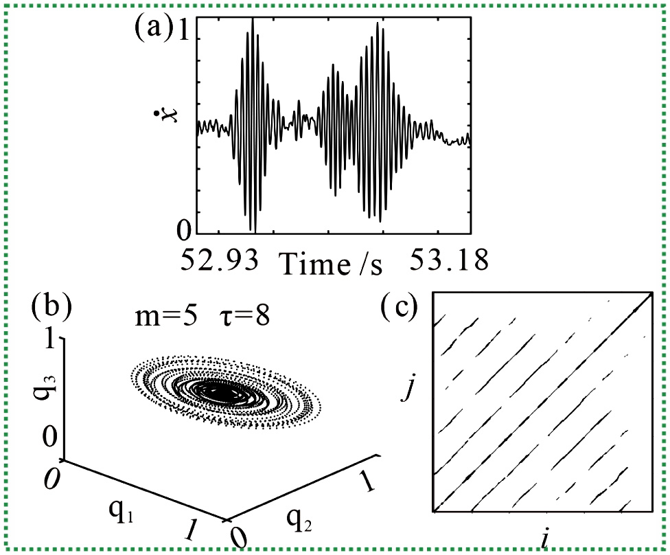 Fig. 16. Phase space analysis reconstruction results of B stage of Case IV.
1)PHASE SPACE RECONSTRUCTION ANALYSIS RESULTS OF CASE I
The results of A stage of Case I (52·5 s∼52·75-s velocity time series in Fig. 7) are shown in Fig. 12(a)–(c). The obtained parameters are m = 2 and τ = 19 for this part. As shown in Fig. 12(a), the velocity in time domain shows sudden jumps, which indicates that the relative motion is slip motion at this time, but stick motion in other time. In the reconstructed orbital diagram in Fig. 12(b), the orbit is evenly expanded in the slip stage but is curled up into small black area in the stick stage.
In the RP in Fig. 12(c), separate alternating white and black areas can be found, the white area corresponding to the slip motion, and the black area formed by isolated points, short diagonal lines, and a large number of vertical lines corresponding to the stick motion. Compared with the RP in Figs. 11(c) and 12(c), the black and white areas without a specific shape appear randomly scattered in the RP. However, it should be noted that although the vibration is very complex, its intensity is very low at this stage.
Fig. 12(d)–(f) shows the reconstruction results of B stage of Case I (50·5 s∼50·75-s velocity time series in Fig. 7). The obtained parameters are m = 3 and τ = 16 for this part. The velocity shows high irregularity in Fig. 12(d); the orbit of space phase in Fig. 12(e) is also in a very chaotic state and unpredictable. The RP in Fig. 12(f) shows that the length of diagonal line in the RP is variable, and the shorter the length of diagonal line, the more irregular the vibration of the system.
The results of Case I further indicate that the friction system exhibit stick-slip vibration in A (decreasing) stage, and low-intensity random vibration in B (increasing) stage. The relative motion between the pad and the disc alternatively switches between stick-slip motion in the decreasing stage of the normal force and stick motion in the increasing stage of the normal force.
2)PHASE SPACE RECONSTRUCTION ANALYSIS RESULTS OF CASE II
The phase space reconstruction results of A stage of Case II (51·8 s∼51·43 s velocity time series in Fig. 7) are shown in Fig. 13(a)–(c). The obtained parameters are m = 3 and τ = 14 for this stage. Three cycles of stick-slip vibration can be seen in Fig. 13(a). The orbital diagram in the three-dimensional phase space also shows two phenomena: uniform expansion and aggregation in Fig. 13(b). The black and white areas in the RP in Fig. 13(c) are no longer blocky areas, but banded areas parallel to the diagonal line. The black area is composed of many short diagonal lines which are parallel to the diagonal line; this phenomenon indicates that the speed signal has certain determinism as time changes.
The phase space reconstruction results of B stage of Case II (52·22 s∼52·47 s velocity time series in Fig. 7) are shown in Fig. 13(d)–(f). The calculated parameters are m = 3 and τ = 15 for this stage. Compared with the velocity in Fig. 12(d), the velocity amplitude is slightly higher in Fig. 13(d). The orbital diagram in the three-dimensional phase space in Fig. 13(e) evolves into a twisted ring shape with many trajectory points clustered in the center of the ring. The RP in Fig. 13(f) shows that length of the short diagonal lines paralleling to the diagonal line is slightly longer compared with that in Fig. 12(f), which indicates that the vibration of the friction system in the stick stage shows higher regularity.
The phase space reconstruction results of Case II show that the stick-slip vibration and stick motion can be found at the A (decreasing) and B (increasing) stages of harmonic normal force, respectively.
3)PHASE SPACE RECONSTRUCTION ANALYSIS RESULTS OF CASE III
For Case III, the phase space reconstruction analysis is performed on the velocity time series of A stage at 51·37 ∼ 51·62 s. The results are shown in Fig. 14(a)–(c). The calculated parameters are m = 7 and τ = 5 for this stage. It can be found that the velocity undergoes four sudden jumps in 0·25 s. The orbital diagram in the three-dimensional phase space also shows similar trend with that of Case I and Case II: uniform expansion and aggregation. The white area in the RP is further enlarged and the black area representing the irregular vibration becomes smaller.
The results of phase space reconstruction analysis of B stage at 51·84 ∼ 52·09 s are presented in Fig. 14(d)–(f). The obtained parameters are m = 3 and τ = 14 for this stage. The amplitude of velocity further increases. The ring shape formed with locus of points in phase space becomes more obvious in the three-dimensional phase space. There are still many single isolated points in the RP, indicating that the friction system has strong oscillation. The single recursive point appears beside the long diagonal line, indicating that there are also unstable periodic trajectories in the friction system. The stick-slip vibration still exists for Case III, but the vibration amplitude in the stick stage increases further.
4)PHASE SPACE RECONSTRUCTION ANALYSIS RESULTS OF CASE IV
The phase space reconstruction results of A stage of Case IV (52·68 ∼52·93 s velocity time series in Fig. 7) are shown in Fig. 15. The calculated parameters are m = 9 and τ = 4 for this stage. The velocity in Fig. 15(a) is much more complex, compared with those of Case I, Case II, and Case III. There are now strong oscillation and sudden jumps of high magnitude in the velocity. The orbital diagram in the three-dimensional phase space shows two different trajectories: high frequency for the red rings marked as H-F FIV and low frequency for the blue droplets marked as L-F FIV, as shown in Fig. 15(b).
An FFT analysis performed for A stage reveals that the main low and high frequencies are respectively 36 Hz and 216 Hz. Considering the fact that the vibration in this stage is quite complex, the velocity in a short time (in the red rectangle in Fig. 15(a)) is used for the RP, and the result is shown in Fig. 15(d). It shows the black area which is similar to that in Fig. 11(c), and some short lines that are parallel to the diagonal line, which further indicates that there is mixed vibration in this stage.
The phase space reconstruction results of the velocity in B stage of Case IV (52·93 ∼53·18 s velocity time series in Fig. 7) are shown in Fig. 16. The calculated parameters are m = 5 and τ = 8 for this stage. It can be found that the velocity shows obvious oscillation with time. The orbit in the three-dimensional phase space (in Fig. 16(b)) is unfolded as concentric ellipses.
To further investigate the dynamic behavior of the friction system in this stage, the velocity with high amplitude in the red rectangle in Fig. 16(a) is selected for phase space reconstruction analysis. The RP in Fig. 16(c) shows only some discontinuous lines parallel to the diagonal line and the distance between each pair of adjacent lines looks same, but no vertical line can be found, which indicates considerable amplitude modulation in the FIV [30]. The phase space reconstruction results of B stage show that the vibration is very stable in this stage; the relative motion between the pad and the disc is slip motion.
V.CONCLUSIONS
In this work, the effects of constant and harmonic normal forces on FIV are investigated. The magnitudes of the constant normal forces are 160 N, 180 N, and 200 N, respectively. For the harmonic normal forces, forcing frequencies of 0·25 Hz, 0·5 Hz, 1 Hz, and 2 Hz are applied, respectively. Phase space reconstruction analysis, PCA, and recurrence analysis are conducted to discover the science behind the complicated dynamic behavior. The main conclusions are as follows:
- (1)Steady stick-slip vibration can be found when the friction system is subjected to a constant normal force. Its intensity increases with the increasing magnitude of the normal force, while its frequency is also affected by the normal force magnitude, in a limited way.
- (2)The harmonic normal force with a different forcing frequency exerts various influences on FIV. The experimental results show that stick-slip vibration occurs in the decreasing stage of the normal force, and stick motion occurs in the increasing stage of the normal force when the normal force oscillation frequencies are 0·25 Hz, 0·5 Hz, and 1 Hz. The intensity of FIV does not show a significant difference under these frequencies, but the frequency components of the resulting FIV differ considerably from each other. The frequency components of the resulting FIV differ considerably from each other, and new and high frequency components emerge with the increase of the oscillation frequency of the harmonic normal force, reflected by the frequent and irregular fluctuation events in the FIV. The theoretical results also show the stick-slip vibration in the decreasing force stage and stick motion in the increasing stage. Furthermore, the FIV is more regular with higher normal force oscillation frequency in its increasing stage.
- (3)At the forcing frequency of 2 Hz, the FIV is fairly complex, as experimental results and the three-dimensional phase space plots and RPs all show that the friction system undergoes wide-frequency vibration in the decreasing stage of the normal force and pure slip motion in the increasing stage of the normal force.
- (4)These results suggest new ways of controlling FIV in engineering, like introducing an appropriate harmonic normal force into an oil well-drilling system and a noisy automobile brake system in order to impede and suppress unwanted stick-slip oscillation. A main challenge of doing this is the actual implementation of this control device in a real machine, such as space restriction and cost.