I.INTRODUCTION
Grinding is the last manufacturing process which is used in situations where sufficient measurement precision and surface quality cannot be produced with other machining methods such as turning, milling, reaming, etc. During grinding, material removal is achieved by the cutting edges of grains of hard material during which are randomly shaped and arranged. These cutting edges penetrate only a few micrometers into the material and cause the formation of large cutting forces which lead to elastic and plastic deformations in the workpiece [1]. In addition, a number of physical phenomena occur including shearing, material removal, friction, heat generation, deformation, fluid flow, etc. The main concern in the grinding process is the harmful effects of high temperatures on the workpiece and tool. Grinding temperatures are the consequences of many factors including the type of workpiece material, the nature of abrasive employed in the grinding wheel, application of grinding fluid, grinding speeds and feeds, and wheel dressing conditions [2]. Since grinding is a finishing process and is usually the last stage of the manufacturing, any damage induced to the workpiece could be very costly and have a major impact on the service life of the product.
A large number of research studies on tool condition monitoring have been reported in the literature for a variety of machining processes by measuring parameters such as force and torque, feed and spindle motor currents, acoustic emissions (AEs), vibration, cutting temperature, etc [3–8]. Of these parameters, AE has been widely used and recognized as one of the most suitable choices for grinding process monitoring. The use of AE is highly desirable due to its superior signal-to-noise ratio and sensitivity which lead to the detection of different levels of AE activities occurring even at very low depths of cut. Another advantage is that the AE sensors generally operate within a frequency range of 50 kHz–1000 kHz that is well above the characteristic frequencies attributed to the machining or natural frequencies of the structure, which minimizes noise in the resulting AE signal [3].
Han et al. [5] studied characteristics of AE in precision grinding under different working conditions and justifications were made by considering root mean square (RMS) and frequency spectrum of AE signal. Karpuschewsk et al. [6] investigated the influence of different dressing parameters on the AE signal, and wheel life estimation was achieved using power spectra of the enveloped AE signal. Plaza et al. [7] carried out an experimental study on AE features in abrasive grinding. The AE signals were analyzed in both the time and frequency domains. It was found that the AE features in the frequency up to 200 kHz could be an ideal data source for the online monitoring of surface creation in grinding processes.
Lezanski [8] monitored grinding wheel wear by measuring vibration, AE, and grinding forces, and the condition of the grinding wheel was assessed using a neural network-based fuzzy logic decision system. Susic et al. [9] investigated the properties of a ground surface using AE signals and the condition of the grinding wheel was estimated using neural network application.
Liu et al. [10] investigated the AE features of the thermal expansion in grinding using wavelet packet transform. Their findings revealed that signal energy at high temperatures was concentrated in the high-frequency bands, whereas it shifted to the low-frequency bands with the reduction of temperature. Kwak et al. [11] carried out a work in which wavelet transform was used for both feature extraction and de-noising of force signal obtained from the grinding process. Liao [12] investigated feature extraction and future selection issues in AE sensor-based condition monitoring of a grinding wheel in which both time series modeling and discrete wavelet decomposition were employed for feature extraction. Yang et al. [13] examined the AE activities from a grinding wheel using both the discrete wavelet transform and support vector machine. RMS and variance from each decomposition level were considered as the feature vector for the classification of sharp and worn wheels. Viera et al. [14] monitored the surface quality of ceramic components during the surface grinding process using the piezoelectric diaphragm and AE sensors. A time domain metric, based on short-time Fourier transform, was employed to assess surface roughness. Hübner et al. [15] investigated the surface integrity of steel during grinding using the AE and electromechanical impedance signals. The resulting AE signals were analyzed using both the short-time Fourier transform and continuous wavelet transform (CWT).
Barkhausen noise (BN) and AE are frequently used approaches to detect thermally induced changes on the surface of a workpiece in grinding. BN analysis is a nondestructive method that involves measuring a noise-like signal induced in a ferromagnetic material by an applied magnetic field and is mostly affected by hardness and stress. Since the grinding burn causes local dislocations on the surface and can soften or harden the surface layer, any thermally induced damage can be detected by the BN analysis [16]. Sorsa et al. [17] used the BN signal to detect residual stress and hardness change due to surface burning in hardened steel. Aguiar et al. [18] investigated the efficiency of some statistical analysis methods in the detection of thermal damages in the grinding process using AE signals. Kwak et al. [19] investigated the chatter vibration and grinding burn in a cylindrical plunge grinding process, and various parameters of raw AE signal were used as burn features for the neural network. Inasaki [20] conducted an experimental study in which the grinding power was monitored to detect grinding burn and found that grinding power increases rapidly when a grinding burn occurs. Yang et al. [21] conducted a work in order to detect surface burn in grinding and used the ensemble empirical mode decomposition (EEMD) method to the resulting AE signal.
Although there are several methods available for feature extraction and prediction in the grinding burn detection, researchers have not reached a consensus on which feature (or features) reflects the nature of grinding burn, and conflicts still arise among the researchers [21]. The main reason for the conflicts is either due to the complex nature of the abrasive process or features extracted using different methods may be effective in their circumstances. It is for these reasons, this study aims to give a new perspective on grinding burn detection using the instantaneous features (i.e., in stantaneous energy and signal phase) of AE derived from the scalogram which is the absolute value of the CWT. Feature extraction using the CWT can be performed with ridge detection [22,23] or low-order conditional moments [24,25]. Because the CWT decomposes the signal into its components, the ridge subtraction method is useful for characterizing the signal components. On the other hand, low-order frequency moments of an energy density function are effective tools for reducing dimensionality and enable the capture of changes in a signal with relatively few parameters, and facilitating the distinction of different fault conditions.
This paper presents the use of low-order frequency moments (i.e., instantaneous energy and mean frequency) of a spectrogram in the detection of thermal damage to the workpiece under different operating conditions in grinding. Firstly, a brief theoretical background is given for the scalogram and its frequency moments. Secondly, the state of the grinding process is monitored for a variety of operating conditions, including the regular grinding, grinding at a higher cutting speed, larger infeed, and smaller dressing depth of cut using AE. Instantaneous features of the AE signal are obtained using the scalogram. In addition, the Hilbert–Huang transform (HHT) and empirical mode decomposition (EMD), whose theoretical bases are detailed in [21,26], are used to demonstrate the effectiveness and efficiency. It has been found that the AE is very sensitive to any change in operating conditions, and the AE power is effective in the frequency range up to 180 kHz for all grindings conditions. Moreover, when the workpiece is burn-damaged, the strength of the resulting AE generally tends to be reduced compared to undamaged conditions for all grinding conditions. Furthermore, both the instantaneous energy and phase deviation serve as robust and reliable indicators by always yielding lower values than those of the undamaged conditions, providing a basis for detecting the burn damage in grinding.
II.METHODS
A.CONTINUOUS WAVELET TRANSFORM (CWT)
CWT is a method that converts a one-dimensional function into a two-dimensional function represented by scale and expansion parameters and is used to measure the similarity between the processed signal and the analysis function. In contrast to Fourier analysis, the wavelet transform performs a decomposition of into a set of waves (or wavelets) which are derived from a single wavelet, termed the analyzing wavelet h(t). The expansion of the signal into wavelets is called the CWT and is defined as follows [27]:
where h(t) is the wavelet kernel function (or mother wavelet) along with the continuous scaling parameter a and the time-shifting parameter b. The interpretation of equation (1) is that the size of the wavelet functions varies with dilation (or scaling) a. When large scales are selected, the resulting wavelet becomes low-frequency wavelet functions and spread out in time, and vice versa.The wavelet transform can be implemented either in the time domain or in the frequency domain. Since the time domain calculation is a convolution operation, it brings a higher computational load. In contrast, a fast calculation of the wavelet transform can be achieved via simple multiplication operations if the frequency domain expression is considered [28]. That is,
where and denote the Fourier transforms of and , respectively, represents the inverse Fourier transform and * indicates the complex conjugation. The fast calculation of the CWT is based on octave band analysis in which each octave is equally subdivided into voices [29]. Although the number of octaves used in the wavelet calculation is dictated by the length of the data time record, the selection of the number of voices depends on the desired frequency resolution of the transform, and the larger the number of voices the better the frequency resolution.Mathematically, the wavelet transform offers flexibility in the selection of the analzsing wavelet. The Morlet wavelet is used in this study because it is closely related to Fourier analysis and is therefore easier to understand. The Morlet wavelet in the time and frequency domains is defined as follows:
where f0 is the wavelet center (or oscillation) frequency and t∈ℜ. The Morlet wavelet itself is not admissible, but appropriate selection of the wavelet center frequency (e.g., ) makes the Morlet wavelet admissible in practice [30].B.SCALOGRAM AND ITS MEAN FREQUENCY
Frequency moments of a distribution are the average spectral properties of a signal and are used to characterize the distribution with few parameters. Using the CWT, an energy density function, which yields time-dependent energy content of a signal over a range of frequencies, can be obtained by computing the scalogram (i.e., the square of the absolute value of the CWT). Signal energy is preserved by the scalogram and can be obtained by integrating scalogram over the whole (b-a) plane. That is,
where denotes the admissibility condition expressed as follows:where is the Fourier transform of h(t). Once the scalogram of a signal is defined, its frequency moments at a particular time t can be expressed as follows:where n () denotes the order of frequency moment. It can be seen that the 0th order moment gives the instantaneous signal energy . That is,The first-order frequency moment of an energy density normalized by at a given time gives the instantaneous (or mean/average) frequency (IF) at which the instantaneous spectra concentrate. The IF, which physically represents the energy center of gravity at a certain time b, can be expressed as follows (see Appendix for its derivation):
where denotes the wavelet center frequency in rad/sec. It can be seen from equation (8) that the IF is meaningful only for those b for which , which is always satisfied by the scalogram. Although the signal phase can be calculated simply by integrating the IF without the need to unwrap, errors in the mean frequency can propagate and affect the accuracy of the phase estimation [31]. In order to precisely estimate the IF features, the important aspect to be considered is that the time-frequency method used can achieve a high time-frequency resolution. The CWT is a linear transform which process the signal through the inner product with a base and which possesses the capability to locate time and frequency. However, the CWT fails to achieve an arbitrarily high time-frequency resolution simultaneously. The bandwidth of the wavelets varies proportionally to their center frequencies, which are adversely affected with the dilation and results in a better localization. As the scale reduces, the wavelets become more compact in time, improving the time resolution of the transform, but frequency resolution deteriorates according to the uncertainty principle [27].III.NUMERICAL VALIDATION AND PERFORMANCE ASSESSMENT
A linear chirp signal was used to demonstrate the effectiveness of the scalogram’s phase recovery and feature extraction capabilities, and the results were compared with those of the EMD for performance evaluation. Simulated signal sampled at 128 Hz and produced for 2 seconds is given by:
The simulated signal was also assumed to be contaminated by a zero-mean random component with a signal to noise ratio of 10 dB. For the scalogram calculation, the Morlet wavelet with a center frequency of was selected, and to avoid a high calculation load, the octave band-based fast calculation procedure was performed using 10 voices per octave.
Fig. 1 shows the test signal together with its scalogram, HHT, and phase information. In the scalogram representation, a path that follows the maximum energy density is termed as a wavelet ridge and the values of along this path give the IF. Since the IF of the noiseless test signal is , the wavelet ridge varies linearly with time. The IF estimated by the first-order frequency moment of the scalogram is also superimposed on the scalogram as a thick red line, which is located exactly on the ridge, indicating a precise estimation of the mean frequency. Figure 1(d) shows the HHT of the noisy chirps (the estimated IF is also superimposed on the HHT) and Fig. 1(e) depicts errors in the estimated instantaneous frequencies compared to the noiseless chirp. It can be seen that the EMD-based IF is heavily affected by noise and yields a choppy appearance. Fig. 1(f) shows the recovered and analytically calculated (or exact) signal phase variations, and a good agreement among them is observed. It can be concluded that the mean frequency of a scalogram can be used to precisely recover the signal phase even when the noise is present.
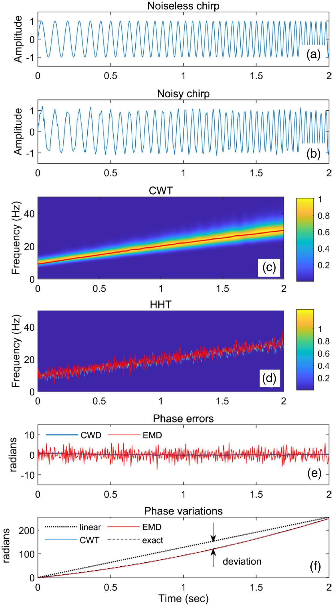 Fig.1. Simulated signal and its scalogram, HHT, and phase information.
IV.EXPERIMENTAL RESULTS
A.EXPERIMENTAL SETUP AND PROCESS PARAMETERS
All the experiments were carried out on a plunge-type CNC cylindrical grinding machine shown in Fig. 2. The workpiece used for the experiments was the outer ring of the 6806 ball bearing and its raceway was ground. It was made of DIN 100Cr6 steel and case-hardened to a depth of 0·15 mm at 60HRc. A vitrified-bond aluminum oxide grinding wheel of diameter 30 mm was used together with a 4% water-soluble coolant.
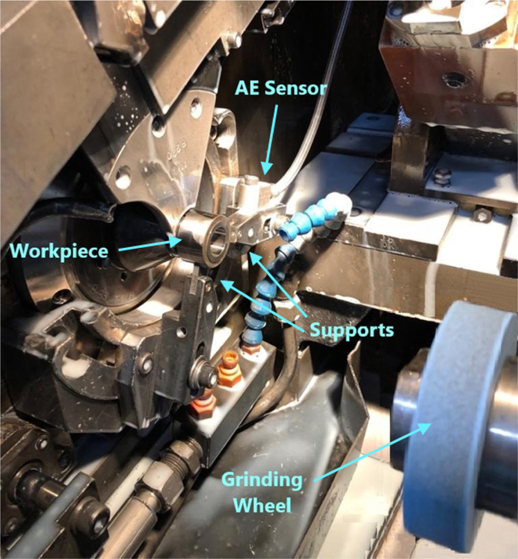 Fig. 2. Plunge-type CNC cylindrical grinding machine.
The condition of the grinding process was monitored for four different cases: normal grinding, grinding with higher cutting speed and larger infeed, and small dressing depth of cut. During the experiments, the workpiece speed was set to 900 rpm for all cutting conditions. For normal grinding test, the circumferential speeds of the grinding wheel and infeed rate were selected as 57 m/sec at 36300 rpm and 0·16 mm/sec, respectively. When a higher cutting speed is applied, the peripheral speed of grinding wheel was increased to 62 m/sec without changing the infeed rate. For the larger infeed case, the infeed rate was raised to 0·3 mm/sec without altering the cutting speed. For all the cases mentioned, the grinding wheel was subjected to a redressing with a depth of 0·03 mm after every six workpieces were ground. In the last experiment, the dressing depth of cut was reduced to 0·010 mm without changing both the cutting speed and infeed rate. The process parameters used for the tests are given in Table I.
Table I. Process parameters used for the grinding tests
| Regular | High cutting speed | Large infeed | Small dressing depth of cut | |
|---|---|---|---|---|
| Peripheral speed (m/sec) | 57 | 62 | 57 | 57 |
| Workpiece speed (rev/min) | 900 | 900 | 900 | 900 |
| Infeed rate (mm/sec) | 0·16 | 0·16 | 0·30 | 0·16 |
| Redressing depth (mm) | 0·03 | 0·03 | 0·03 | 0·01 |
An AE sensor, Kistler type 8152C, was used to capture the resulting AE activities. During the experiments, the obtained AE signals were sampled at 2 MHz and captured for a complete grinding process, including idles before and after the grinding period. A built-in anti-aliasing filter on data acquisition board was used to avoid aliasing effect. For each grinding operation, three AE data were selected for each of the healthy and burned states, and the instantaneous frequencies from these data were averaged to increase the reliability. For the scalogram analysis, the wavelet center frequency was selected, and to avoid a high calculation load, the octave band-based fast calculation procedure was performed using 10 voices per octave.
B.REGULAR GRINDING
Figure 3 shows the AE signal obtained during normal grinding and its spectra for idle and cutting periods. It can be seen that the amplitude of AE signal exhibits a regular increase in the early phase of the grinding and then remains almost unchanged until the end of the roughing period. This is because that the actual depth of cut gradually increases until the specified depth is approached. This hence causes a continuous increase in undeformed chip thickness (and consequently in cutting force) which leads to larger deformation and raises the strength of AE.
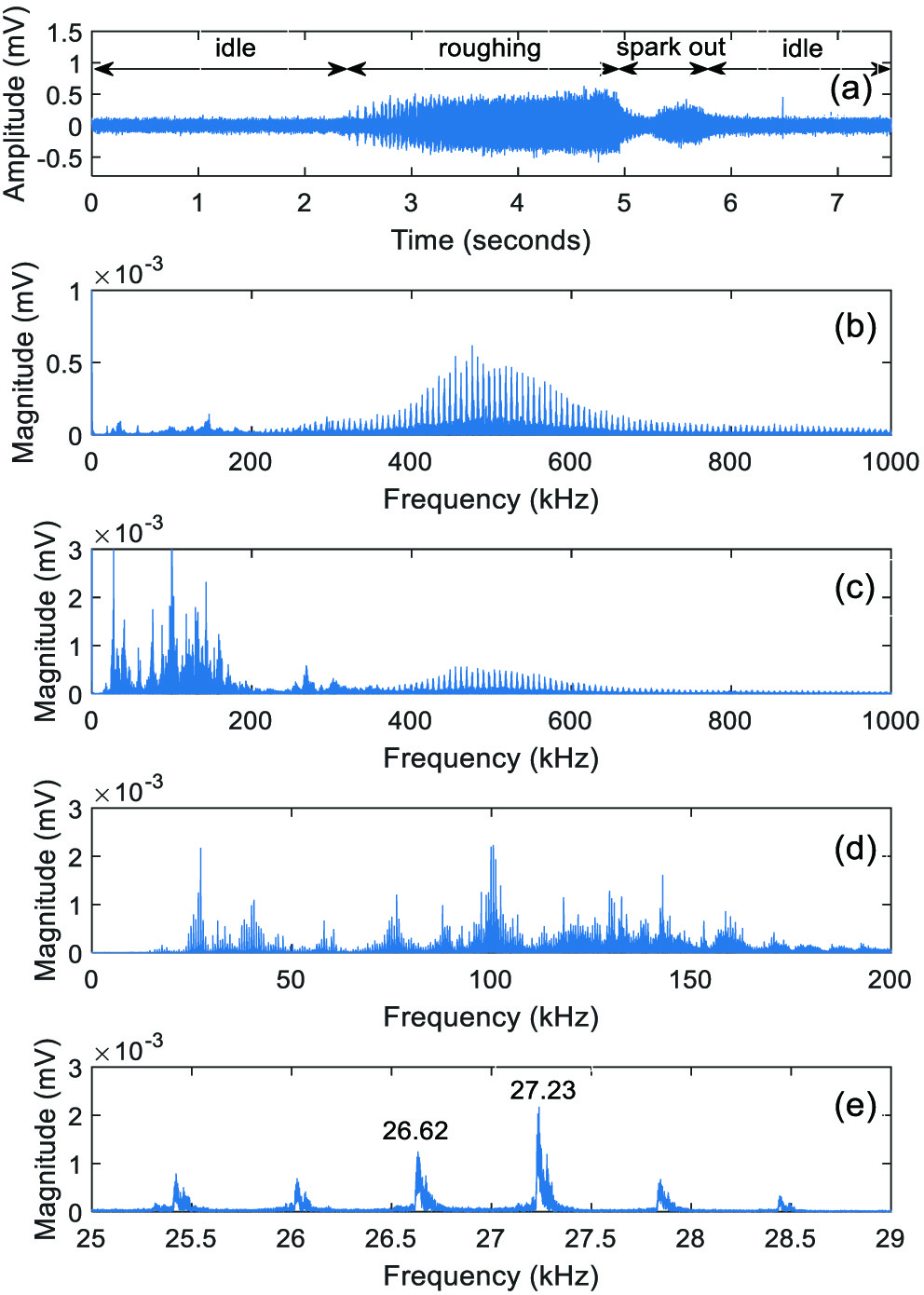 Fig. 3. (a) Raw AE signal for the regular grinding, (b) magnified spectrum of AE signal for the idle period, (c) spectrum of AE signal for the cutting period, (d) spectrum of the filtered AE signal, and (e) zoomed spectrum of the filtered AE signal around 27 kHz.
The idle period spectrum exhibits a periodic frequency activity centered around 500 kHz and its extensions can be seen in the region from 200 kHz to 1 MHz, and this can be considered as the reflection of machine-related events on the AE signal. In contrast, the cutting period spectrum reveals that most of the condition indicating information for the grinding process is seen in the low-frequency region up to 200 kHz. This is because small cutting grains are randomly shaped and distributed in the grinding wheel, and after resurfacing or dressing, hundreds or thousands of grains likewise appear on the cutting surface of the grinding wheel. Since the grinding process requires a very high cutting speed, high-frequency events occur due to the frictional interaction of these grains with the workpiece. Therefore, all the AE signals obtained during the experiments were band-pass filtered on computer by a 10th-order elliptic filter whose cutoff frequencies are set at 3 kHz and 200 kHz to avoid machine-related frequency activities and noise.
The spectrum of the filtered AE signal exhibits nonperiodic frequency activities up to 200 kHz, with the most pronounced peaks seen at 27·2 kHz and 99·8 kHz, and a large number of sidebands also become apparent around these frequency peaks. When the spectrum is zoomed around its peak at 27 kHz, sidebands appear 605 Hz (i.e. 36300 rpm) apart from each other. These sideband peaks are caused by errors such as imbalance or eccentricity of the grinding wheel and occur at all frequencies.
Figure 4 comparatively shows the CWT and HHT of the AE signal for the regular grinding with its instantaneous properties. Since the frequency resolution of the CWT deteriorates with increasing frequency, the high-frequency components cannot be discernible on the scalogram. However, the energy and frequency features of the AE signal can be extracted by the zero- and first-order frequency moments of the scalogram as shown in Fig. 4(c) and (d). It is seen that both the scalogram and EMD give the same IE values and the mean frequencies obtained are almost the same. Although the resulting phase changes appear reasonably linear, the phase extracted from the scalogram exhibits a peak-to-peak deviation of 12818 radians, while EMD analysis yields a larger phase deviation of 18896 radians. The scalogram and EMD-based phase deviations of the AE signals for different grinding conditions are given in Table II.
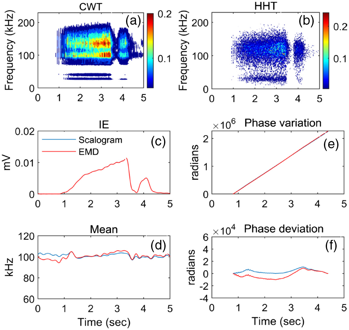 Fig. 4. (a) CWT and (b) HHT of the AE signal for the regular grinding, (c) estimated instantaneous energy and (d) mean frequency variations, (e) signal phases, and (f) phase deviations for the cutting period.
Table II. RMS and phase deviation values of the AE signals obtained in the healthy and burnt conditions for different grinding conditions
| Regular | High cutting speed | Large infeed | Small dressing depth of cut | |||||
|---|---|---|---|---|---|---|---|---|
| Intact | Intact | Burn | Intact | Burn | Intact | Burn | ||
| RMS | 0·074 | 0·048 | 0·040 | 0·077 | 0·076 | 0·107 | 0·102 | |
| Phase deviation (radians) | Scalogram | 10778 | 57647 | 31006 | 43723 | 28343 | 30234 | 14054 |
| EMD | 18896 | 65137 | 26087 | 55744 | 27872 | 41717 | 16388 |
C.GRINDING AT A HIGHER CUTTING SPEED
Figure 5 shows the time, frequency, CWT, and HHT representations of the AE signals for the healthy and burnt conditions when the cutting speed is set to 62 m/s. Although the time trace of the AE signal obtained in the healthy state is very similar to that of the regular grinding, it exhibits a lesser amplitude variation and yields a smaller RMS value as given in Table II (only the grinding period has been considered for the calculations of RMS). This is mainly because that the undeformed chip thickness (and hence the cutting force) decreases with increasing wheel speed, resulting in smaller deformation and decreasing the strength of AE [5]. Increasing the cutting speed is also very effective on the frequency content of the AE signal. Compared to normal grinding, the frequency positions of the peaks are not changed, but their amplitudes are significantly reduced. When the workpiece is burn damaged, the amplitude of the resulting AE signal is further diminished.
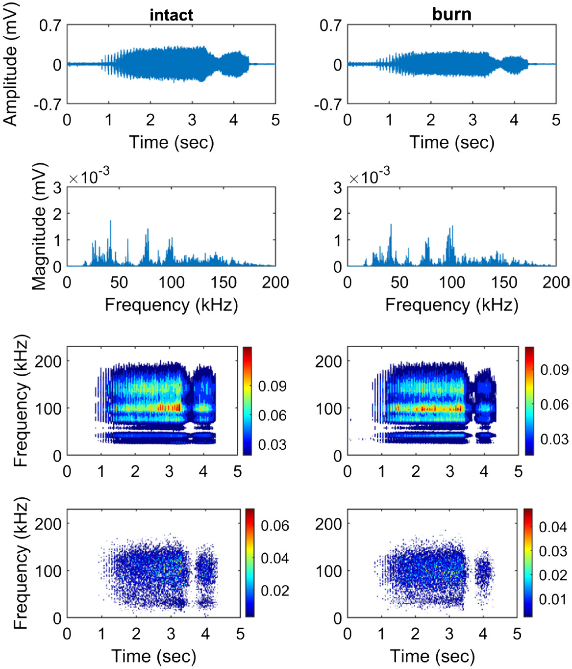 Fig. 5. Time, frequency, CWT, and HHT representations of the AE signals for the healthy and burn conditions when a higher cutting speed is applied.
Figure 6 illustrates the scalogram and EMD-based instantaneous features of the AE signals for the intact and burnt conditions. As with regular grinding, both the scalogram and the EMD give the same IE values and provide very similar mean frequency variations. Although the IE for the burnt case diminishes noticeably, the mean frequency exhibits a slight reduction during the roughing period compared to the intact condition. In addition, the signal phase for the burnt case exhibits a lesser deviation than that of the undamaged condition. Figure 7 shows the raceway surfaces of healthy and burnt bearing parts after grinding, where burn damage manifests itself in the form of localized black spots on the raceway.
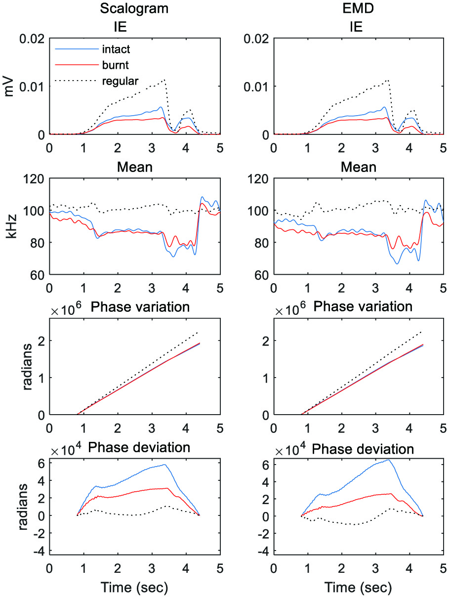 Fig. 6. Scalogram (first column) and EMD (second column)-based instantaneous characteristics of the AE signals for health and burnt conditions when a higher wheel speed is applied.
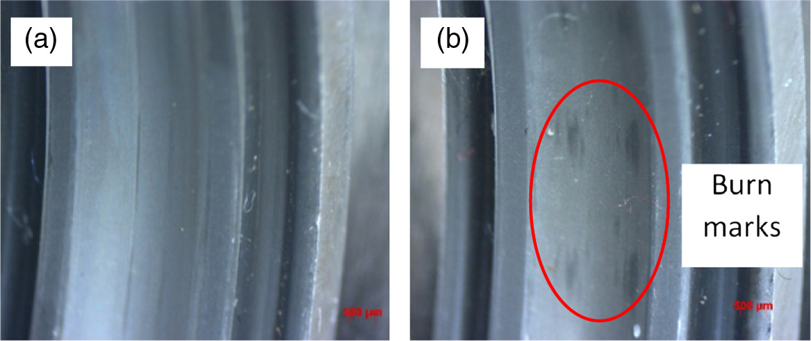 Fig. 7. Raceway surfaces of the healthy and burnt bearing parts after grinding (a) intact and (b) burnt.
D.GRINDING AT A LARGER INFEED RATE
Figure 8 illustrates the time and frequency, CWT, and HHT representations of the AE signals for the healthy and burnt conditions when the infeed rate is raised from 0·16 mm/sec to 0·3 mm/sec. Compared to regular grinding, increasing the feed rate reduces the roughing time but increases the amplitude of the AE. The main reason for this is that as the feed rate increases, the undeformed chip thickness increases and accordingly, more cutting force and large deformations occur. This ultimately leads to an increase in both the number of active particles in contact with the workpiece and the strength of AE activities. When the workpiece is thermally damaged, the signal energy is slightly reduced compared to the undamaged condition, as given in Table II. As with higher wheel speed, the application of a larger infeed in intact or burnt states does not affect the positions of the resulting frequency activities, but their strength is significantly affected.
 Fig. 8. Time, frequency, CWT, and HHT representations of the AE signals for the healthy and burn conditions when a larger infeed is applied.
Figure 9 shows the instantaneous features derived from the scalogram and EMD of AE signals for healthy and burnt conditions when the infeed rate is increased. As in the case of higher wheel speed, the scalogram and EMD provide almost the same instantaneous characteristics, and the presence of burn damage often causes reductions in both the IE and IF values during the roughing period. Also, in the burnt condition, the phase of the AE signal deviates less than in the undamaged condition.
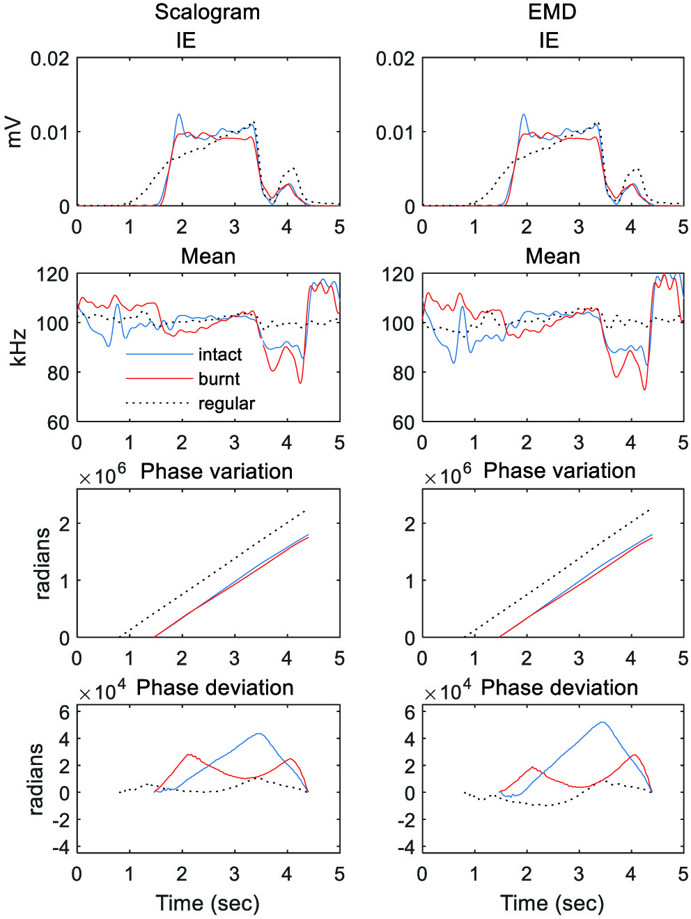 Fig. 9. Scalogram (first column) and EMD (second column)-based instantaneous characteristics of the AE signals for health and burnt conditions when a larger infeed is applied.
E.GRINDING AT A SMALLER DRESSING DEPTH OF CUT
During the experiments, the grinding wheel was resurfaced using a single-point sharpening tool after every six workpieces were ground, and the dressing depth of cut and dressing feed per revolution were selected as 0·03 mm and 0·22 mm/rev, respectively. However, the dressing depth of cut was reduced to 0·01 mm without changing the dressing feed to examine whether a finer dressing condition has an effect on burn formation. Figure 10 shows the time and frequency, CWT, and HHT representations of the AE activities for the healthy and burn conditions when the dressing depth of cut is reduced to 0·01 mm. It can be seen that the AE in the healthy state shows larger amplitude variations than in regular grinding. That is because more cutting edges on the wheel surface emerge when a fine dressing condition is applied. However, the presence of more cutting edges does not necessarily provide an effective cutting action in terms of lower cutting force and finer surface [32]. In addition, fine dressing tends to produce a matte wheel and causes cracks in grains on the cutting surface [2]. As a result, the grinding process, taking place immediately after a fine dressing operation, causes an increase in grinding power and cutting forces and consequently strengthens the resulting AE activity. When the workpiece is burnt, there is no readily discernible difference between the time traces of the AE signals obtained for the healthy and burn conditions and this is likewise indicated by the RMS values. In the frequency domain, the application of a smaller dressing depth of cut does not change the positions of the frequency peaks again, but their strength is significantly affected in both grinding conditions.
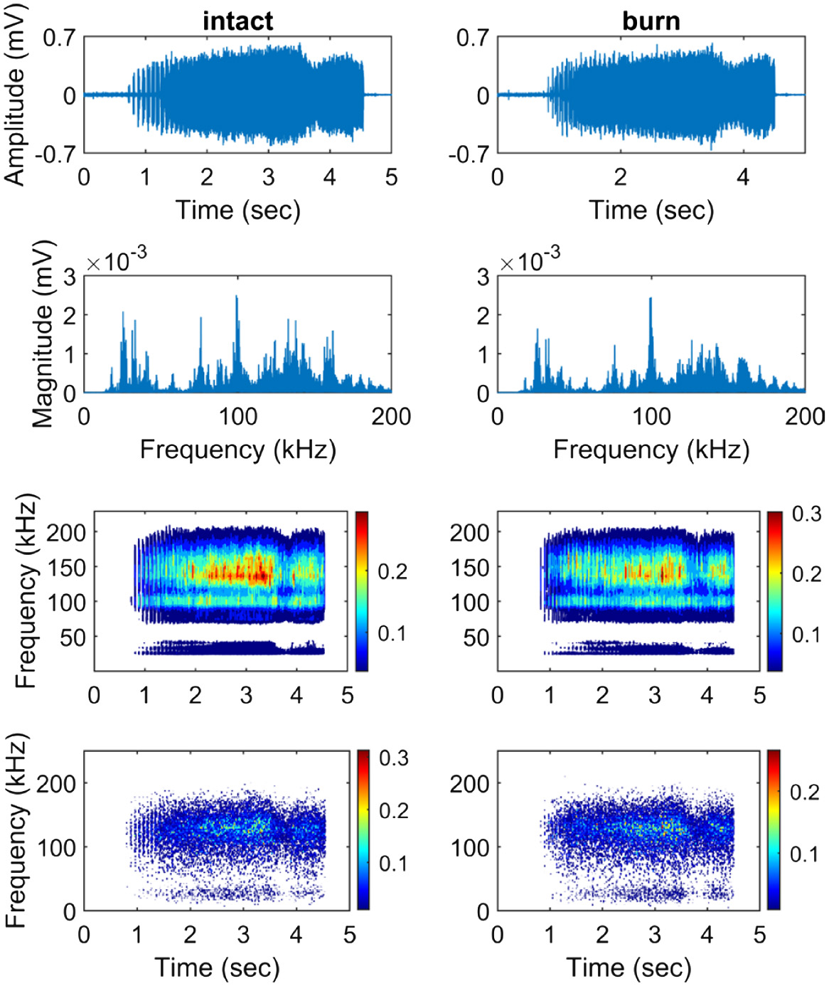 Fig. 10. Time, frequency, CWT, and HHT representations of the AE signals for the healthy and burn conditions when a smaller dressing depth of cut is applied.
Figure 11 shows the scalogram and EMD-based instantaneous features of the AE signals for the intact and burnt conditions when the dressing depth of cut is reduced to 0·01 mm. Applying a smaller depth of cut makes the values of both the IE and mean frequency larger than those of the regular grinding. As with the higher wheel speed and greater infeed cases, the presence of burn damage causes a reduction in the IE values and yields a lesser deviation in phase than those of the intact condition during the grinding period.
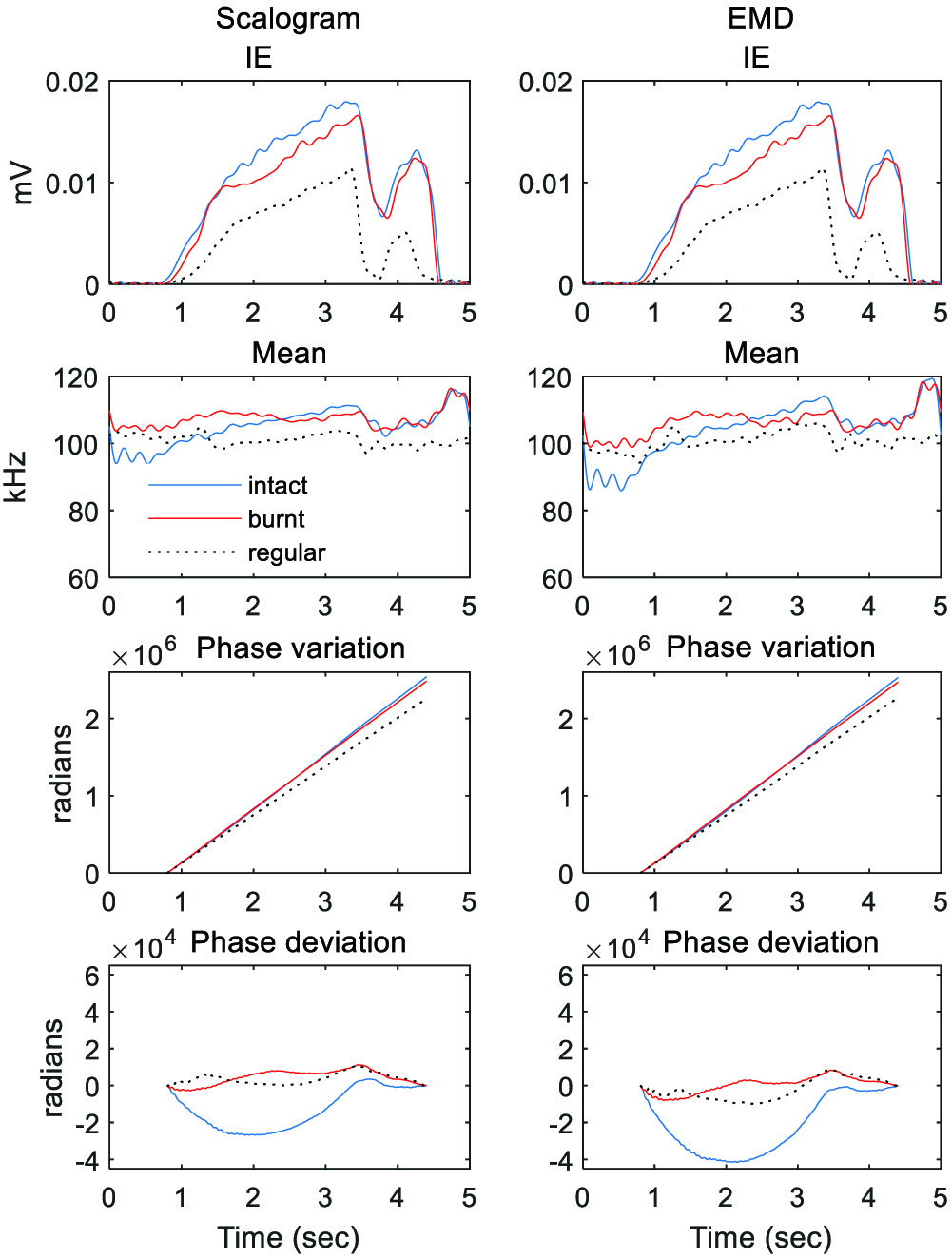 Fig. 11. Scalogram (first column) and EMD (second column)-based instantaneous characteristics of the AE signals for health and burnt conditions when a smaller dressing depth of cut is applied.
V.SUMMARY AND CONCLUSIONS
In this article, scalogram-based instantaneous signal features are used for the detection of burn damage under different grinding operations, and performance assessment is achieved using the EMD. It has been found that AE is very sensitive to any change in operating conditions, and any possible change is evident in the RMS value. The strength of the resulting AE increases as the infeed rate rises or the depth of cut decreases but diminishes when a higher cutting speed is applied. In the frequency domain, the AE energy is seen to be effective in the frequency range up to 180 kHz for all grinding conditions. When the cutting condition changes, the positions of the frequency components remain unchanged, but their power is significantly affected. When the workpiece is thermally damaged, the strength of the AE diminishes compared to the undamaged condition and causes a decrease in RMS values for all grinding operations.
The instantaneous properties of the AE signals are extracted using both the scalogram and the EMD and found that the IE values obtained by both methods are exactly the same, and the recovered mean frequency variations are quite close to each other. It has been found that both the instantaneous energy and phase deviation are found to be quite sensitive to the presence of burn damage. In all grinding operations, the IE values tend to decrease and the signal phase deviates less than in the healthy state when the part is damaged.