JAIT

I.INTRODUCTION

Image denoising methods usually obtain degradation models via $y = x + v$ to recover a clean image $x$ , where $y$ denotes a given noisy image and $v$ is an additive white Gaussian noise of standard deviation $σ$ [1]. According to that, traditional image denoising methods can be divided into spatial pixel feature methods based on filters [2] and transforming domain methods [3] in image denoising. Specifically, the mentioned spatial pixel feature methods based on filters usually use filters (i.e., linear filter [4] and nonlinear filter [5]) to suppress noise for obtaining a latent clean image. Besides, the transforming domain methods [6], priori knowledge [7] and Markov methods [8] were also effective for image denoising. Although these methods have obtained good denoising effects, they are limited by the following aspects. First, they need manual selecting parameters to improve denoising performance. Second, they depended on complex optimization algorithms to improve effects on image denoising.

Deep networks, especially convolutional neural networks (CNNs), are black boxes, which can automatically learn useful information for image denoising [9]. For instance, a denoising CNN (DnCNN) [10] embedded batch normalization (BN) [11] and activation function of ReLU [12] to address the image denoising problem. To reduce the computational cost, noisy mapping and noisy images are cut to patches as inputs of deep network to train a denoiser [13]. To improve the denoising effect, two subnetworks extract complementary features to train a robust denoiser [14]. These CNNs have performed well in image denoising. Also, they show that different components may be useful for image denoising. Inspired by that, we propose a hybrid denoising CNN (HDCNN). HDCNN is composed of a dilated block (DB), RepVGG block (RVB), feature refinement block (FB), and a single convolution. DB combines a dilated convolution, BN, common convolutions, and activation function of ReLU to obtain more context information. RVB uses parallel combination of convolution, BN, and ReLU to extract complementary width features. FB is used to obtain more accurate information via refining obtained feature from the RVB. A single convolution collaborates a residual learning operation to construct a clean image.

This paper has the following contributions:

(1)We use simple components to implement an efficient denoising network.
(2)RVB in a CNN can extract complementary width features in image denoising.
(3)The simultaneous use of serial and parallel architecture to improve denoising performance.
(4)This paper can be used for blind denoising.

The remaining parts of this paper have the following originations.

Section II illustrates related work. Section III gives the proposed method. Section IV shows experiments. Section IV summaries and concludes the whole paper.

II.RELATED WORK

A.DEEP CONVOLUTIONAL NEURAL NETWORKS FOR IMAGE DENOISING

Due to strong expressive abilities, CNNs have been widely used for image restoration [15], such as image denoising [16]. Designing network architecture is effective for image denoising [5]. For instance, Lan et al. [17] fused residual block into a CNN to suppress noise for obtaining clean images. Shi et al. [18] integrated hierarchical features to obtain richer information to improve denoising results. Gai et al. combined a residual CNN, leaky rectified linear units (Leaky ReLU), perceptive loss, and edge information to enhance learning ability of designed denoising network [19]. Mao et al. used an encoder–decoder architecture with skip connections to obtain a symmetric network for mining detailed information in image restoration [20]. Liu et al. [21] used single processing techniques, i.e., wavelet idea and CNN to implement a good performance in image denoising. Inspired by that, we also use deep CNNs for image denoising in this paper.

B.REPVGG

According to VGG, it is known that enlarging the depth of CNN can improve performance in image processing [22]. Alternatively, enlarging the width of CNN (GoogLeNet) can extract more features in image applications [23]. However, deeper CNN may suffer from gradient vanishing or gradient exploding [24]. Also, wider CNN is easier to overfitting [24]. To overcome the phenomenon, He et al. [24] added output of previous layer and output of current layer as output of current layer to implement an efficient CNN (residual CNN) for image recognition. According to mentioned illustrations, Ding et al. used the merits of VGG, GoogLeNet, and residual CNN to obtain a CNN (RepVGG) for making a tradeoff between performance and speed in image recognition [25]. Based on the analysis to the existing work, this paper presents the parallel combination of convolution of $3 \times 3$ , convolution of $1 \times 1$ , and BN to obtain excellent performance in image classification [25], which consumes less memory for real devices. For pursuing better performance, we introduce RepVGG into a CNN for image denoising in this paper.

C.DILATED CONVOLUTION

Although CNNs rely on their layers to extract rich features, interactions of different layers are important for image applications, according to Ref. [24]. Thus, capturing more context information is key to design an efficient CNN. There are two ways to obtain more context information. First, enlarging the depth or width of CNNs can enlarge the receptive field to mine more context features. However, they will increase difficulties of training CNNs, according to the introduction of Section II.B. Furthermore, they may take more memory, which is not suitable to real devices. Thus, the second way is developed. That is, dilated convolution uses dilated factor to obtain more accurate context information for making a tradeoff between performance and computational costs [26,27]. Based on its strong performance, it has been used for image denoising [28].

Tian et al. used dilated convolution into a CNN to train a fast denoiser [29]. Trung et al. combined dilated convolution, BN, perceptual loss, and CNN to obtain clean CT images, which can provide the help for doctors [30]. According to these explanations, we can see that dilated convolution is very suitable in image denoising. Thus, we can use dilated convolution in a CNN to suppress noise in this paper.

III.THE PROPOSED METHOD

A.NETWORK ARCHITECTURE

We propose a 34-layer hybrid DnCNN containing DB, RVB, FB, and a single convolution. DB combines dilated convolutions, BN, common convolution, and activation function of ReLU to obtain more context information. RVB uses parallel combination of convolution, BN and ReLU, to extract complementary width features. FB is used to obtain more accurate information via refining obtained feature from the RVB. A single convolution collaborates a residual learning operation to construct a clean image. To clearly show the process of the designed HDCNN in Fig. 1, we use an equation to present mentioned illustrations as follows:

I_{c} = H D C N N (I_{n}) = I_{n} - C (F B (R V B (D B (I_{n})))),

(1)

where HDCNN denotes the function of HDCNN,

I_{c}

and

I_{n}

are a precited clean image and given noisy image, respectively. DB, RVB, FB, and C express functions of DB, RVB, FB, and a single convolution, respectively. Additionally, “-” is a residual operation, which is equal to

\oplus

in Fig. 1. Parameters of HDCNN can obtained by Section III.B.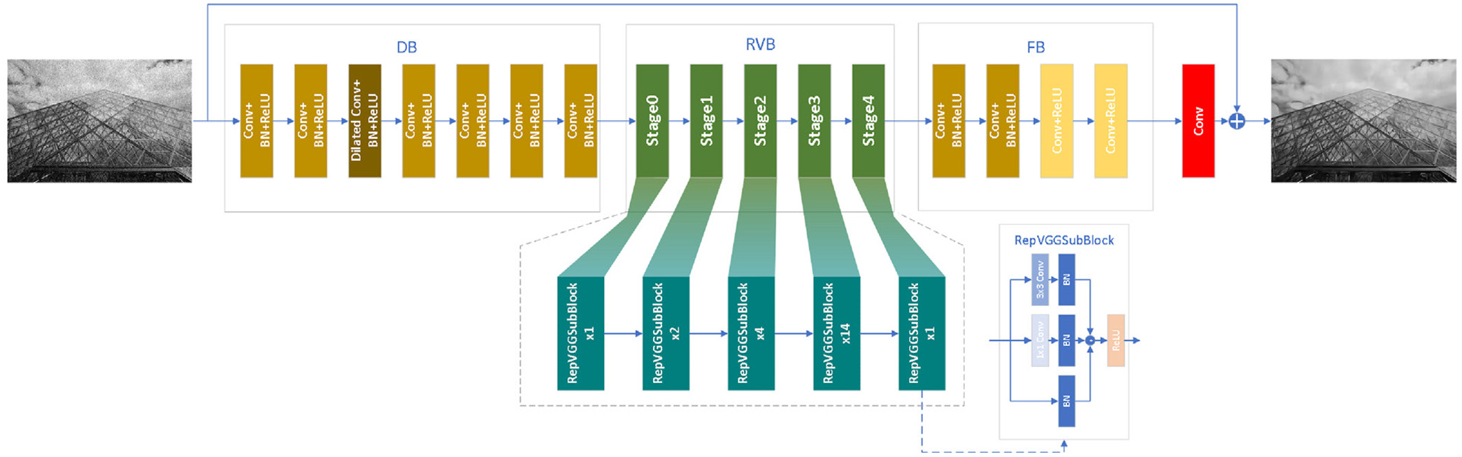

Fig. 1. Network architecture of the proposed HDCNN.

B.LOSS FUNCTION

The HDCNN is trained by the loss function of mean square error (MSE) [31] and training pairs ${I_{n}^{i}, I_{C}^{i}}$ , where $I_{n}^{i}$ and $I_{C}^{i}$ denote the $i th$ noisy image and reference clean image, $i = 1, 2, 3, 4, \dots N$ and N stands for the number of noisy images. This process can be formulated as Eq. (2).

l (θ) = \frac{1}{2 N} \sum_{i = 1}^{N} ‖ H D C N N (I_{n}^{i}) - I_{C}^{i} ‖^{2},

(2)

where

θ

is the parameter set and

l

is the loss function. Besides, parameters of training process can be optimized via Adam [32].

C.DILATED BLOCK

The DB consists of 7 layers, which are used to obtain more context information. The 1st, 2nd, 4th, 5th, 6th, and 7th layers are composed of Conv+BN + ReLU, which is equal to the combination of a convolutional layer, BN, and ReLU. The 3rd layer includes a dilated convolution, BN, and ReLU, which is also represented as dilated Conv+BN + ReLU. The dilated convolution is used to obtain more context information [26]. BN can accelerate the training speed [11]. ReLU is used to transform linear features to nonlinearity [12]. And input and channel number of the 1st layer are 3 and 64, respectively. Input and channel numbers besides the 1st layer in the DB are 64. Sizes of all the kernels are $3 \times 3$ . The mentioned procedure can be shown as Eq. (3).

O_{D B} = D B (I_{n}) = R B C (R B C (R B C (R B C (R B D C (R B C (R B C (I_{n}))))))),

(3)

where RBC denotes the Conv+BN + ReLU and RBDC is dilated Conv+BN + ReLU.

O_{D B}

is the output of DB, which acts RVB.

D.REPVGG BLOCK

The 22-layer RVB uses a parallel mechanism to obtain complementary features. The parallel mechanism contains 22 RepVGG subblocks, and each RepVGG subblock contains three paths of BN, $3 \times 3$ Conv+BN, and $1 \times 1$ Conv+BN. It outputs three paths, and they can be fused via a residual operation. Subsequently, it acts as a ReLU. Specifically, $3 \times 3$ Conv+BN denotes a combination of a convolution layer with $3 \times 3$ and BN. $1 \times 1$ Conv+BN is a combination of a convolution layer with $1 \times 1$ . Input and output channel numbers of all the layers are 64. The introduction above can be explained as follows:

O_{R V B} = R V B (O_{D B}) = 22 R e p V G G S u b B l o c k (O_{D B}),

(4)

R e p V G G S u b B l o c k (x) = R (B (x) + B C (x) + B C_{1} (x)),

(5)

where 22RepVGGSubBlock denotes 22 stacked RepVGG subblocks. We assume that

x

is the input of RepVGGSubBlock.

E.FEATURE REFINEMENT BLOCK

The 4-layer FB uses two types to obtain more accurate information. The first type is Conv+BN + ReLU, which is used as the first and second layers in the feature refinement block. The second type is Conv+ReLU, which is used as the third and fourth layers in the feature refinement block. Conv+ReLU denotes the combination of a convolution layer and ReLU. And its channel number of their inputs and outputs is 64. Sizes of their kernels are $3 \times 3$ . The description can be shown in Eq. (6).

O_{F B} = F B (O_{R V B}) = R B (R B (R C B (R C B (O_{R V B})))),

(6)

F.CONSTRUCTION CLEAN IMAGES

A single convolution layer and a residual operation are used to construct clean images. Input and output channel numbers are 64 and 3. The mentioned illustrations are as follows Eq. (7).

I_{c} = I_{n} - C (O_{F B}),

(7)

IV.EXPERIMENTS

A.DATA SETS

1)TRAINING DATA SET AND TEST DATA SETS

We use 432 images with size of 481 × 321 from Berkeley Segmentation Data set (BSD) [33] to train a Gaussian synthetic gray image denoising model. To improve training speed, we randomly divide a training image into patches of size $48 \times 48$ . Additionally, each training image is operated via one of eight ways: original image, 90°, 180°, 270°, original image with flopped itself horizontally, 90° with flopped itself horizontally, 180° with flopped itself horizontally, and 270° with flopped itself horizontally.

For test data sets, we use three public data sets, i.e., BSD68 [33] and Set12 [33] to conduct comparative experiments.

B.IMPLEMENTATION DETAILS

The initial parameters are learning rate of 1e-4, batch size of 64, patch size of 48, and the number of epochs is 50. The learning rates vary from 1e-4 to 1e-7 for 50 epochs. That is, learning rates from the 1st to the 20th epochs are 1e-4. Learning rates from the 21th to the 35th epochs are 1e-5. Learning rates from the 36th to the 45th epochs are 1e-6. Learning rates from the 46th to the 50th epochs are 1e-7. And other parameters can refer to Ref. [34].

We apply Pytorch 1.10.2 [35] and Python 3.8.12 to implement codes of HDCNN. Specifically, all the experiments are conducted on the Ubuntu 20.04.2 with two Intel(R) Xeon(R) Silver 4210 CPU @ 2.20GHz, RAM 128G, and four Nvidia GeForce GTX 3090 GPU. Finally, the Nvidia CUDA of 11.1 and cuDNN of 8.0.4 are used to accelerate the training speed of GPU.

C.NETWORK ANALYSIS

To test the validity of key techniques in the proposed method, we designed the following experiments. As shown in Table I, we can see that HDCNN outperforms HDCNN without DB on BSD68 for $σ = 15$ , which shows that DB is effective for image denoising. HDCNN has obtained higher PSNR value than that of HDCNN without RVB, which tests the effectiveness of RVB in image denoising. HDCNN is superior to HDCNN without FB, which verifies the effectiveness of FB in image denoising. HDCNN exceeds HDCNN without BN, which shows the effectiveness of BN for image denoising. HDCNN has obtained better performance than that of HDCNN without dilated convolution, which tests the effectiveness of dilated convolution for image denoising.

Table I PSNR (dB) results of several networks from BSD68 with σ=15

Methods	PSNR (dB)
HDCNN	31.74
HDCNN without FB	31.61
HDCNN without RVB	31.62
HDCNN without dilated convolution	31.74
HDCNN without BN	31.69
HDCNN without DB	31.73

According to mentioned illustrations, we can see the effectiveness of key components in the HDCNN for image denoising.

D.COMPARISONS WITH STATE-OF-THE-ART DENOISING METHODS

We use qualitative and quantitative analysis to test the performance of HDCNN for image denoising. In terms of qualitative analysis, we use popular denoising methods, i.e., block-matching and 3-D filtering (BM3D) [36], weighted nuclear norm minimization (WNNM) [37], expected patch loglikelihood (EPLL) [38], trainable nonlinear reaction diffusion (TNRD) [39], DnCNN [10], image restoration CNN (IRCNN) [40], fast and flexible denoising convolutional neural network (FFDNet) [13], and enhanced CNN denoising network (ECNDNet) [29] as comparative methods on BSD68 and Set12 to conduct experiments. Specifically, we use noise levels from 0 to 55 on BSD68 and Set12 to train a blind denoising.

In terms of quantitative analysis, we use predicted clean images of different methods on Set12 for $σ = 15$ and $σ = 25$ to enlarge an area as observation area, where observation areas are clearer, their corresponding methods have better denoising performance. Detailed analysis of mentioned illustrations is shown as follows.

As shown in Table II, we can see that the proposed method has obtained the best denoising results on BSD68 for $σ = 15$ and $σ = 25$ . Also, it has obtained the second best denoising results on BSD68 for $σ = 50$ . Blind denoising network as well as HDCNN-B is competitive to other poplar denoising method, i.e., TNRD. Besides, HDCNN and HDCNN-B are effective for single noisy image denoising, as shown in Table III. For instance, our HDCNN has obtained the best result for image denoising in Table III. The best and second denoising are marked by red and blue lines, respectively. As mentioned in Introduction section, our HDCNN is effective for image denoising and blind denoising in terms of qualitative analysis.

Table II Average PSNR (dB) of different methods on BSD68 with different noise levels of 15, 25, wand 50

Methods	BM3D[36]	WNNM[37]	EPLL[38]	TNRD[39]	DnCNN[10]	IRCNN[40]	FFDNet[13]	ECNDNet[29]	HDCNN	HDCNN-B
σ = 15	31.07	31.37	31.21	31.42	31.72	31.63	31.62	31.71	31.74	31.43
σ = 25	28.57	28.83	28.68	28.92	29.23	29.15	29.19	29.22	29.25	28.96
σ = 50	25.62	25.87	25.67	25.97	26.23	26.19	26.30	26.23	26.23	25.98

Table III Average PSNR (dB) results of different methods on Set12 with noise levels of 15, 25, and 50

Images	C.man	House	Peppers	Starfish	Monarch	Airplane	Parrot	Lena	Barbara	Boat	Man	Couple	Average
Noise Level	σ = 15
BM3D[36]	31.91	34.93	32.69	31.14	31.85	31.07	31.37	34.26	33.10	32.13	31.92	32.10	32.37
WNNM[37]	32.17	35.13	32.99	31.82	32.71	31.39	31.62	34.27	33.60	32.27	32.11	32.17	32.70
EPLL[38]	31.85	34.17	32.64	31.13	32.10	31.19	31.42	33.92	31.38	31.93	32.00	31.93	32.14
TNRD[39]	32.19	34.53	33.04	31.75	32.56	31.46	31.63	34.24	32.13	32.14	32.23	32.11	32.50
DnCNN[10]	32.61	34.97	33.30	32.20	33.09	31.70	31.83	34.62	32.64	32.42	32.46	32.47	32.86
IRCNN[40]	32.55	34.89	33.31	32.02	32.82	31.70	31.84	34.53	32.43	32.34	32.40	32.40	32.77
ECNDNet[13]	32.56	34.97	33.25	32.17	33.11	31.70	31.82	34.52	32.41	32.37	32.39	32.39	32.81
HDCNN	32.51	35.17	33.22	32.23	33.20	31.69	31.86	34.57	32.60	32.39	32.36	32.46	32.86
HDCNN-B	31.87	34.67	32.79	31.87	32.62	31.38	31.56	34.27	31.80	32.11	32.20	32.12	32.44
Noise Level	σ = 25
BM3D[36]	29.45	32.85	30.16	28.56	29.25	28.42	28.93	32.07	30.71	29.90	29.61	29.71	29.97
WNNM[37]	29.64	33.22	30.42	29.03	29.84	28.69	29.15	32.24	31.24	30.03	29.76	29.82	30.26
EPLL[38]	29.26	32.17	30.17	28.51	29.39	28.61	28.95	31.73	28.61	29.74	29.66	29.53	29.69
TNRD[39]	29.72	32.53	30.57	29.02	29.85	28.88	29.18	32.00	29.41	29.91	29.87	29.71	30.06
DnCNN[10]	30.18	33.06	30.87	29.41	30.28	29.13	29.43	32.44	30.00	30.32	30.10	30.12	30.43
IRCNN[40]	30.08	33.06	30.88	29.27	30.09	29.12	29.47	32.43	29.92	30.17	30.04	30.08	30.38
ECNDNet[13]	30.11	33.08	30.85	29.43	30.30	29.07	29.38	32.38	29.84	30.14	30.03	30.03	30.39
HDCNN	30.03	33.28	30.75	29.42	30.37	29.11	29.43	32.53	30.03	30.23	30.01	30.14	30.44
HDCNN-B	29.59	32.75	30.55	29.06	30.13	28.88	29.13	32.12	29.17	29.88	29.85	29.77	30.06
Noise Level	σ = 50
BM3D[36]	26.13	29.69	26.68	25.04	25.82	25.10	25.90	29.05	27.22	26.78	26.81	26.46	26.72
WNNM[37]	26.45	30.33	26.95	25.44	26.32	25.42	26.14	29.25	27.79	26.97	26.94	26.64	27.05
EPLL[38]	26.10	29.12	26.80	25.12	25.94	25.31	25.95	28.68	24.83	26.74	26.79	26.30	26.47
TNRD[39]	26.62	29.48	27.10	25.42	26.31	25.59	26.16	28.93	25.70	26.94	26.98	26.50	26.81
DnCNN[10]	27.03	30.00	27.33	25.70	26.78	25.87	26.48	29.39	26.22	27.20	27.24	26.90	27.18
IRCNN[40]	26.88	29.96	27.33	25.57	26.61	25.89	26.55	29.40	26.24	27.17	27.17	26.88	27.14
ECNDNet[13]	27.07	30.12	27.30	25.72	26.82	25.79	26.32	29.29	26.26	27.16	27.11	26.84	27.15
HDCNN	27.20	30.04	27.47	25.73	26.89	25.82	26.29	29.50	26.14	27.16	27.23	26.93	27.20
HDCNN-B	26.55	29.31	26.81	25.32	26.33	25.55	26.18	29.07	25.51	26.87	26.97	26.47	26.75

As shown in Figs. 2 and 3, we can see that the proposed method has obtained clearer images than that of other methods. This shows that our method is competitive with these popular methods for image denoising in terms of quantitative analysis. Besides, we can see that the proposed HDCNN outperforms other denoising methods in Figs. 4 and 5. According to the above descriptions, our method is effective for image denoising and blind denoising.

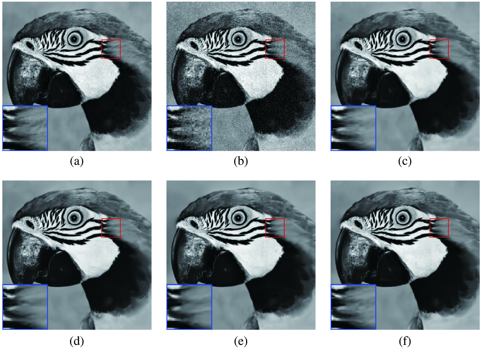Fig. 2. Denoising results of different methods on one image from Set12 with σ = 15. (a) Original image, (b) noisy image, (c) BM3D/31.37, (d) DnCNN/31.83, (e) FFDNet/31.84, (f) HDCNN/31.86.

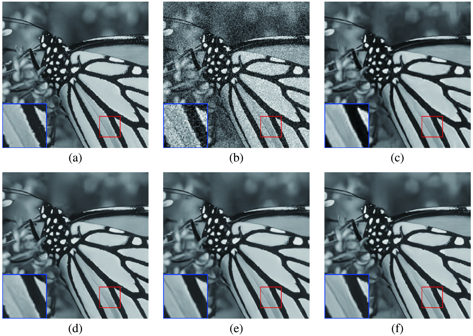Fig. 3. Denoising results of different methods on one image from Set12 with σ = 25. (a) Original image, (b) noisy image (c) BM3D/29.25, (d) DnCNN/30.28, (e) FFDNet/30.31, (f) HDCNN/30.37.

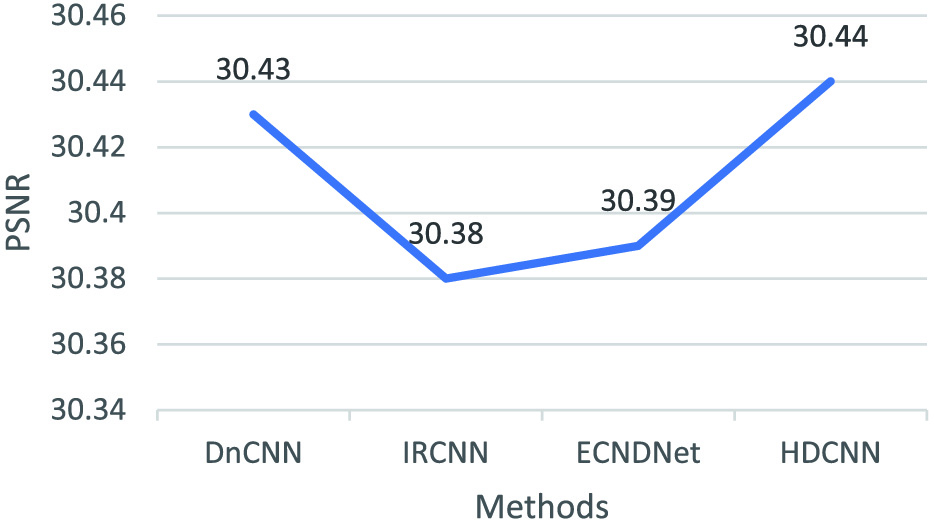Fig. 4. Denoising results of different methods (i.e., DnCNN, IRCNN, ECNDNet, and HDCNN) on Set12 for noise level of 25.

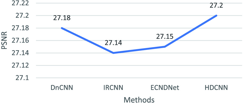Fig. 5. Denoising results of different methods (i.e., DnCNN, IRCNN, ECNDNet, and HDCNN) on Set12 for noise level of 50.

V.CONCLUSIONS

In this paper, we propose a HDCNN, which mainly uses several blocks (i.e., a DB, RVB, and feature refinement block) to implement a robust denoising network. DB is used to obtain more context information via the combination of a dilated convolution, BN, common convolution, and ReLU. RVB is used to obtain extract complementary width features through parallel combination of convolution, BN, and ReLU. FB is used to obtain more accurate information. The simultaneous use of these key components has obtained good performance for image denoising and blind denoising.

A Hybrid CNN for Image Denoising