I.INTRODUCTION
Mangrove forests represent a vital component of tropical and subtropical coastal ecosystems, occupying approximately 14.7 million hectares globally [1]. More than one-third of the world’s mangrove forests are located in Southeast Asia [2,3], where over 46 mangrove species have been identified [3]. Despite their limited spatial extent, these ecosystems deliver critical ecological functions, including nutrient filtration, shoreline stabilization, and carbon sequestration, with an estimated economic value exceeding US$194,000 per hectare annually [4,5]. However, mangrove cover has declined significantly over recent decades due to land-use change, rising sea levels, elevated temperatures, and shifts in rainfall patterns [1,6]. In Indonesia, this degradation has resulted in not only a reduction in forest extent but also a measurable decline in ecosystem health [7].
Monitoring mangrove health is therefore essential for conservation planning and climate change mitigation. The Mangrove Health Index (MHI) provides a reliable, standardized indicator for assessing mangrove ecosystem condition using measurable field parameters such as canopy coverage, stem diameter, and sapling density [8]. Remote sensing and GIS techniques have demonstrated effectiveness in mapping and analyzing mangrove distribution across large spatial extents [9,10]. Medium-resolution satellite data from Landsat 8 and Sentinel-2 have proven particularly useful for identifying mangrove distribution and health status at regional scales [9]. Spectral indices derived from these sensors including the Normalized Difference Vegetation Index (NDVI), Normalized Burn Ratio (NBR), Enhanced Vegetation Index (EVI), Atmospherically Resistant Vegetation Index (ARVI), and Modified Red Edge-Simple Ratio (mRe-SR) have shown strong sensitivity to vegetation condition and canopy structure, making them valuable predictors for mangrove health modeling [11,12].
Machine learning (ML) algorithms have been increasingly integrated with satellite-derived spectral indices to improve vegetation health assessments. Random forest regression (RFR), support vector regression (SVR), and artificial neural network regression (ANNR) were applied to WorldView-2 imagery to estimate the leaf area index (LAI) of mangroves, with RFR achieving the lowest root mean square error (RMSE) of 0.45 [13]. While this study demonstrated the potential of combining spectral indices with ML, it relied on high-resolution commercial imagery and focused on a single biophysical parameter. These constraints limit its scalability for broader, operational ecosystem health monitoring.
Previous MHI studies primarily rely on field surveys or simple optical indices without integrating ML frameworks, which constrains their ability to generalize across large and heterogeneous coastal areas [8,14]. Moreover, systematic comparisons of multiple ML regression models using freely available medium-resolution imagery remain limited in the literature. These gaps highlight the need for a scalable, data-driven approach that produces spatially continuous and ecologically meaningful mangrove health assessments.
This study addresses these limitations by developing a robust MHI prediction framework for Belawan District, North Sumatra. It integrates Sentinel-2 multispectral imagery with three ML algorithms SVR, RFR, and k-nearest neighbor (k-NN) using multiple spectral indices as predictors. Model performance is validated against ground-truth ecological measurements through K-fold cross-validation. The specific contributions of this study are: (1) demonstrating the effectiveness of freely available medium-resolution imagery for operational MHI mapping; (2) providing a comparative evaluation of three ML regression algorithms under a rigorous cross-validation framework; and (3) producing a spatially explicit MHI distribution map applicable to conservation and restoration planning in Belawan District.
II.METHOD
A.STUDY AREA
The specific research site chosen to assess the MHI is the natural mangrove environment located in the Belawan District of Medan, within the North Sumatra Province, as depicted in Fig. 1. The investigation took place between June and November 2023.
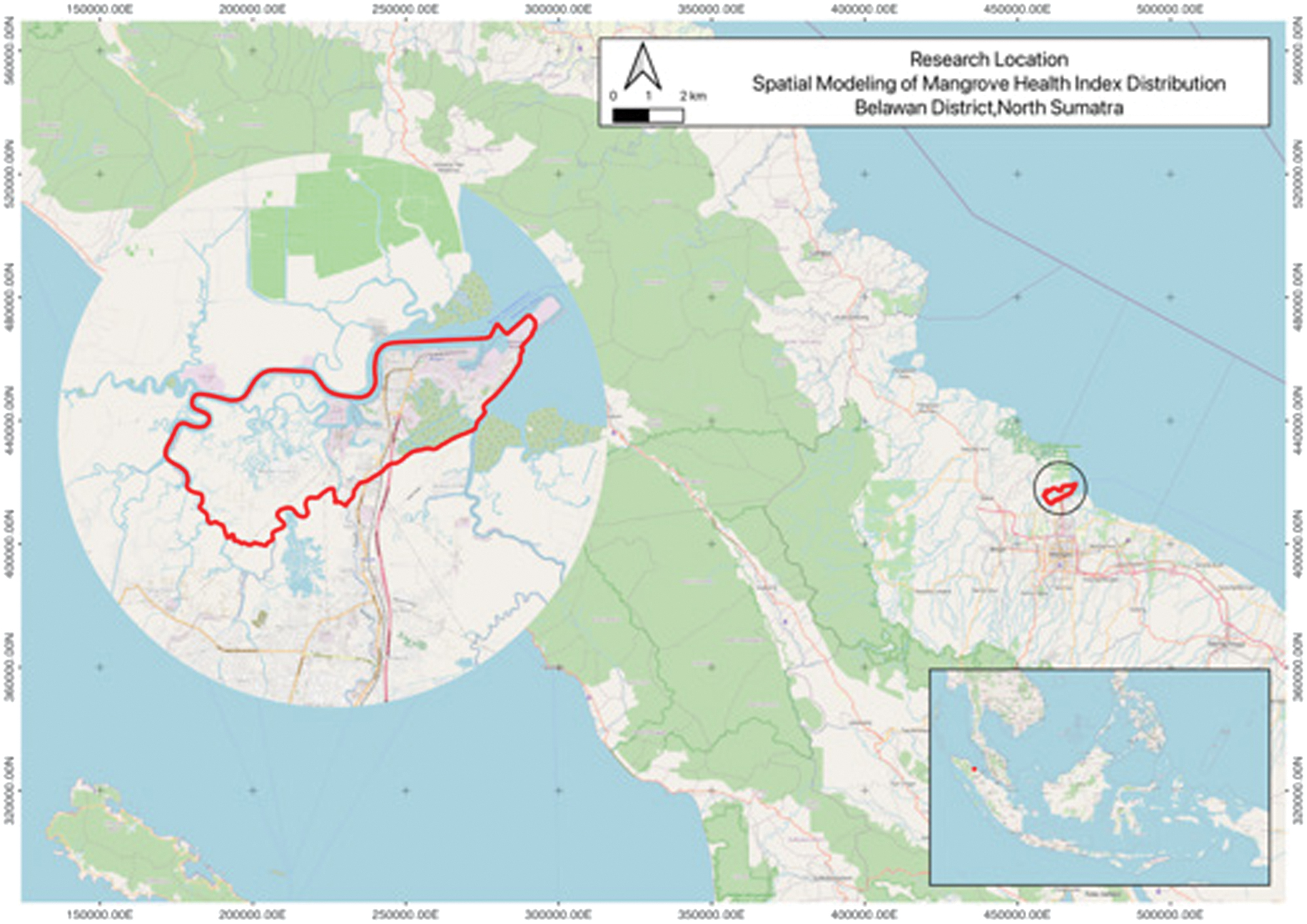 Fig. 1. Study area in Belawan District, North Sumatra, Indonesia.
B.METHODS
The analysis of the MHI involves a multi-stage approach comprising data collection, satellite image preprocessing, spectral index extraction, ML modeling, and model evaluation. Figure 2 illustrates the overall methodological workflow.
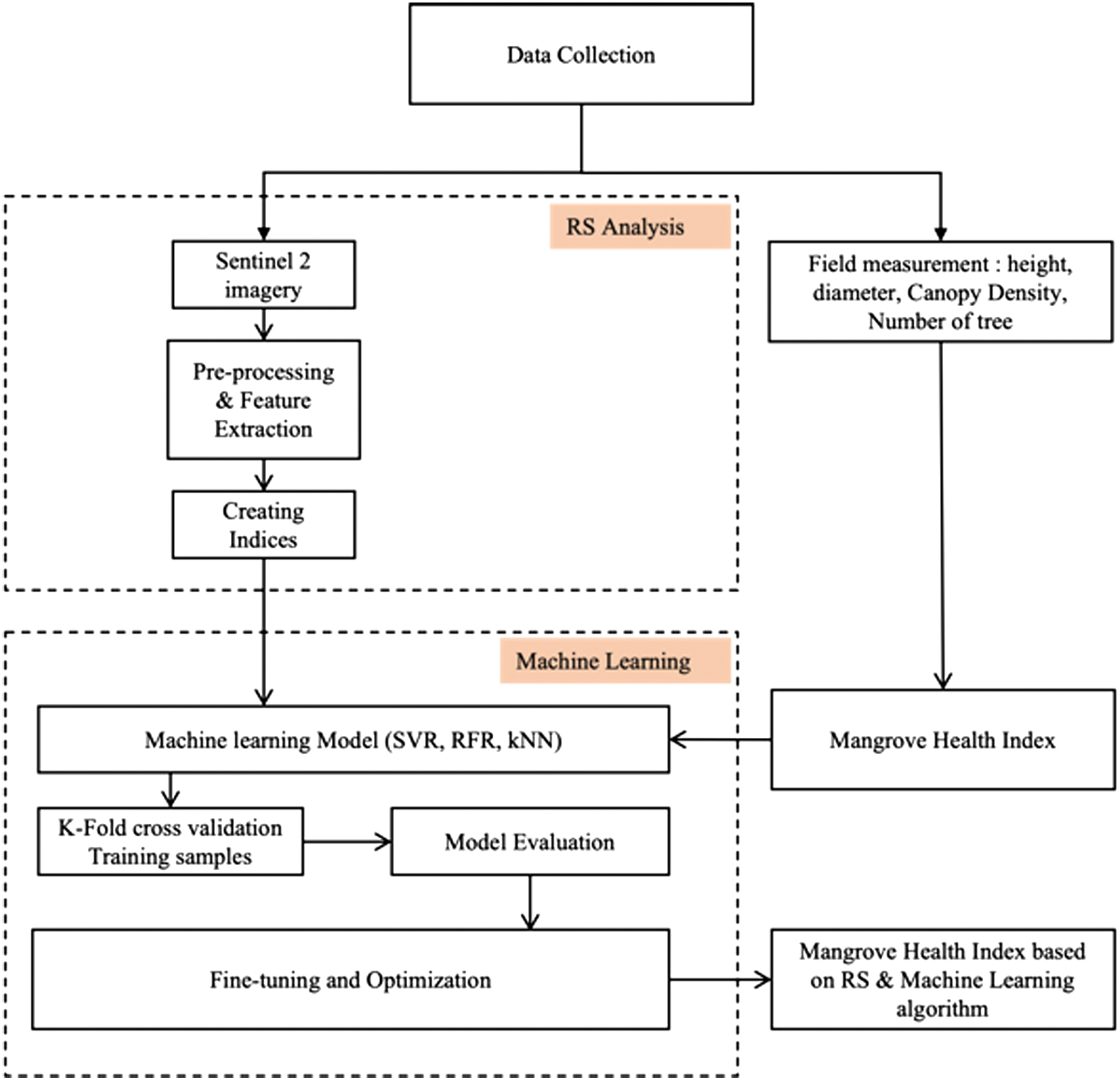 Fig. 2. The flow chart for the estimation of mangrove health using machine learning.
1).DATA COLLECTION
Data acquisition follows a two-stage approach, integrating Sentinel-2 satellite imagery with ground-truth field measurements. Sentinel-2 data were obtained from the Copernicus Open Access Hub https://dataspace.copernicus.eu/. Subsequent ground-truthing involved careful data collection to validate algorithms used in estimating key ecological parameters, including diameter, canopy cover, and sapling density per unit area. These datasets were then used to calculate the MHI, which served as a critical component for field validation of the algorithmic estimates.
- a.Sentinel-2 Imagery Acquisition and PreprocessingSentinel-2 imagery acquired on July 25, 2023 is used in this study. The acquisition date is selected to closely align with the field data collection period. The imagery is obtained at Level-2A processing level from the Copernicus Open Access Hub (https://dataspace.copernicus.eu/), which provides surface reflectance data with atmospheric correction already applied using the Sen2Cor algorithm. Cloud masking is subsequently performed to eliminate pixels contaminated by cloud cover, ensuring data quality across the study area. It is acknowledged that tidal conditions were not explicitly controlled during image acquisition. However, the selected image date corresponds to the dry season, which typically exhibits more stable and lower tidal fluctuations in the Belawan coastal area, minimizing potential tidal influence on spectral values.
- b.Spectral Index ExtractionFollowing preprocessing, five spectral indices are derived from the corrected Sentinel-2 bands to serve as predictor variables for MHI estimation. These indices are selected based on their established sensitivity to vegetation condition and canopy structure in mangrove ecosystems [11,12]. The indices computed are as follows:
- 1.NDVI (Normalized Difference Vegetation Index): captures overall vegetation greenness and density.
- 2.NBR (Normalized Burn Ratio): sensitive to vegetation stress and canopy disturbance.
- 3.EVI (Enhanced Vegetation Index): reduces atmospheric and soil background influences compared to NDVI.
- 4.ARVI (Atmospherically Resistant Vegetation Index): minimizes residual atmospheric effects using blue band correction [14].
- 5.mRe-SR (Modified Red Edge-Simple Ratio): exploits the red-edge band to improve sensitivity to canopy chlorophyll content.
- c.Ground Data CollectionA comprehensive field survey is conducted across 218 sample plots, each measuring 10 × 10 meters. The plots are strategically distributed across the study area and grouped by plant type and canopy density to ensure representation of a wide range of ecological conditions. Three ecological parameters are measured in each plot: stem diameter (measured using a diameter tape), canopy cover percentage, and sapling density per unit area. These parameters are subsequently used to calculate the MHI as the response variable for model training and validation.
2).MANGROVE HEALTH INDEX (MHI)
MHI is defined as a measure that shows, defines, or reflects the health of mangrove forest ecosystems. The health of the mangrove community in Indonesia is evaluated using three key components: natural community metrics, environmental variables, and regeneration. Specific characteristics include substrate type, tree density, canopy coverage, and diameter. The MHI is computed as a percentage by combining canopy coverage, stem diameter, and stakes per area scores. The formula for calculating the MHI is as follows [8].
whereS = score
C = canopy cover percentage (%)
D = stem diameter (stake + trees) (cm)
Nsp = number of stakes per area
The formula for calculating the score of each component is given as:
SC = 0.25 × C-13.06; however, if C < 0, then S_C = 0 and if C > 10, then S_C = 10
SD = 0.45 × D + 1.42; however, if D < 0, then S_D = 0 and if D > 10, then S_D = 10
SNsp = 0.13 × Nsp + 4.1; however, if Nsp < 0, then S_Nsp = 0 and if S_Nsp > 10, then S_Nsp= 10
3).K-FOLD CROSS-VALIDATION
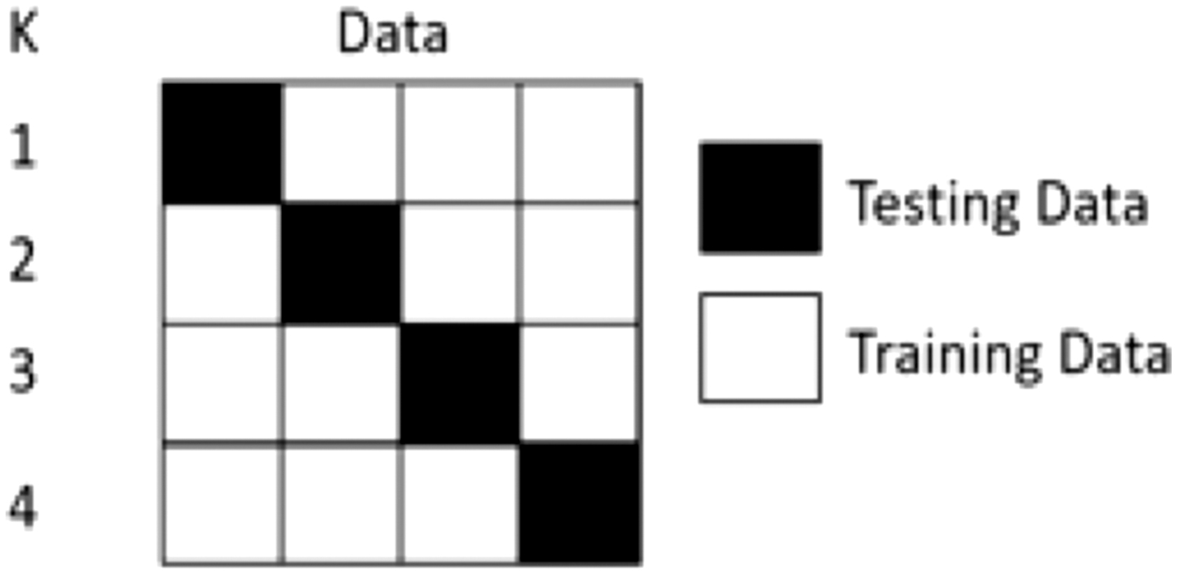
K-fold cross-validation is applied to evaluate model performance on the complete dataset. The dataset is partitioned into K subsets (folds). In each iteration, K-1 folds serve as training data and the remaining fold serves as testing data. This process is repeated K times so that every fold is used once for testing. In this study, K is set to 5, providing a robust and unbiased estimate of model generalization performance [15,16] as illustrated in Fig. 3.
4).SUPPORT VECTOR REGRESSION (SVR)
SVR is a supervised learning algorithm derived from support vector machine (SVM) theory [17]. It estimates a continuous function by fitting an optimal hyperplane that approximates the relationship between input predictors and the target variable within a defined margin of tolerance (ɛ) [18,19]. In this study, SVR is implemented using the radial basis function (RBF) kernel via the svmRadial method in the caret package in R. Predictor variables are standardized through centering and scaling prior to model fitting. Hyperparameter optimization is performed using grid search over two parameters: the kernel width parameter (sigma, ranging from 0.1 to 1.0 with a step of 0.1) and the regularization parameter (C, ranging from 0.1 to 1.0 with a step of 0.1), resulting in 100 candidate combinations. The optimal parameter combination is selected based on the lowest cross-validated RMSE across 5-fold cross-validation.
5).K-NEAREST NEIGHBOR (KNN)
The k-NN is a nonparametric method and the simplest ML algorithm used for both classification and regression [20]. It estimates the target value of a new observation based on the values of its k closest training samples in feature space. The algorithm has been widely applied for estimating forest attributes from remote sensing data [21–24]. In this study, k-NN is implemented using the caret package in R, with predictor variables standardized through centering and scaling. The number of neighbors (k) is optimized through grid search over values ranging from 1 to 10 (step of 1), evaluated under 5-fold cross-validation. The value of k yielding the lowest RMSE is selected as the final model configuration. A smaller k tends to increase variance, while a larger k increases bias [25].
6).RANDOM FOREST REGRESSION (RFR)
Random forest (RF) is an ensemble learning algorithm derived from the Classification and Regression Tree (CART) model [26]. It constructs multiple decision trees, each trained on a randomly drawn bootstrap sample of the training data. Only a random subset of predictor variables is considered at each node split, which reduces correlation among trees and improves generalization [27–29]. The final prediction is obtained by averaging the outputs of all trees. In this study, RFR is implemented using the rf method in the caret package in R, with predictor variables standardized through centering and scaling. Hyperparameter tuning is performed using grid search over the number of variables randomly sampled at each split (mtry), with values ranging from 1 to 10. Model selection is based on the lowest RMSE obtained through 5-fold cross-validation, consistent with the procedure applied to SVR and k-NN.
7).EVALUATION MODEL
The performance and accuracy of the model used to estimate the MHI were evaluated using the RMSE, mean absolute error (MAE), and coefficient of determination (R2). These statistical criteria are widely utilized in modeling in order to determine the differences between the observed data (the MHI inventories) and the predicted MHI data [30,31]:
where and are observed and predicted MHI, respectively, n is the total number of validation samples used, and is the observed mean values of MHI.III.RESULTS
A.MHI ANALYSIS
Ground data collection was used to assess mangrove health using Equation 1. Measurements were conducted across 218 sample plots distributed throughout the area of interest, collecting a varied range of ecological parameters including canopy coverage, stem diameter, and sapling density. The descriptive statistics of the MHI values reveal a mean of 59.31%, with values ranging from poor to excellent health categories. The spatial distribution of MHI calculation results is presented in Fig. 4, revealing that the mangrove health condition is predominantly categorized as moderate (50%), followed by excellent (39%) and poor (11%). Mangrove healthiness is classified into three fundamental categories based on the MHI ranges: poor (0–33%), moderate (33–66%), and excellent (66–100%) [12].
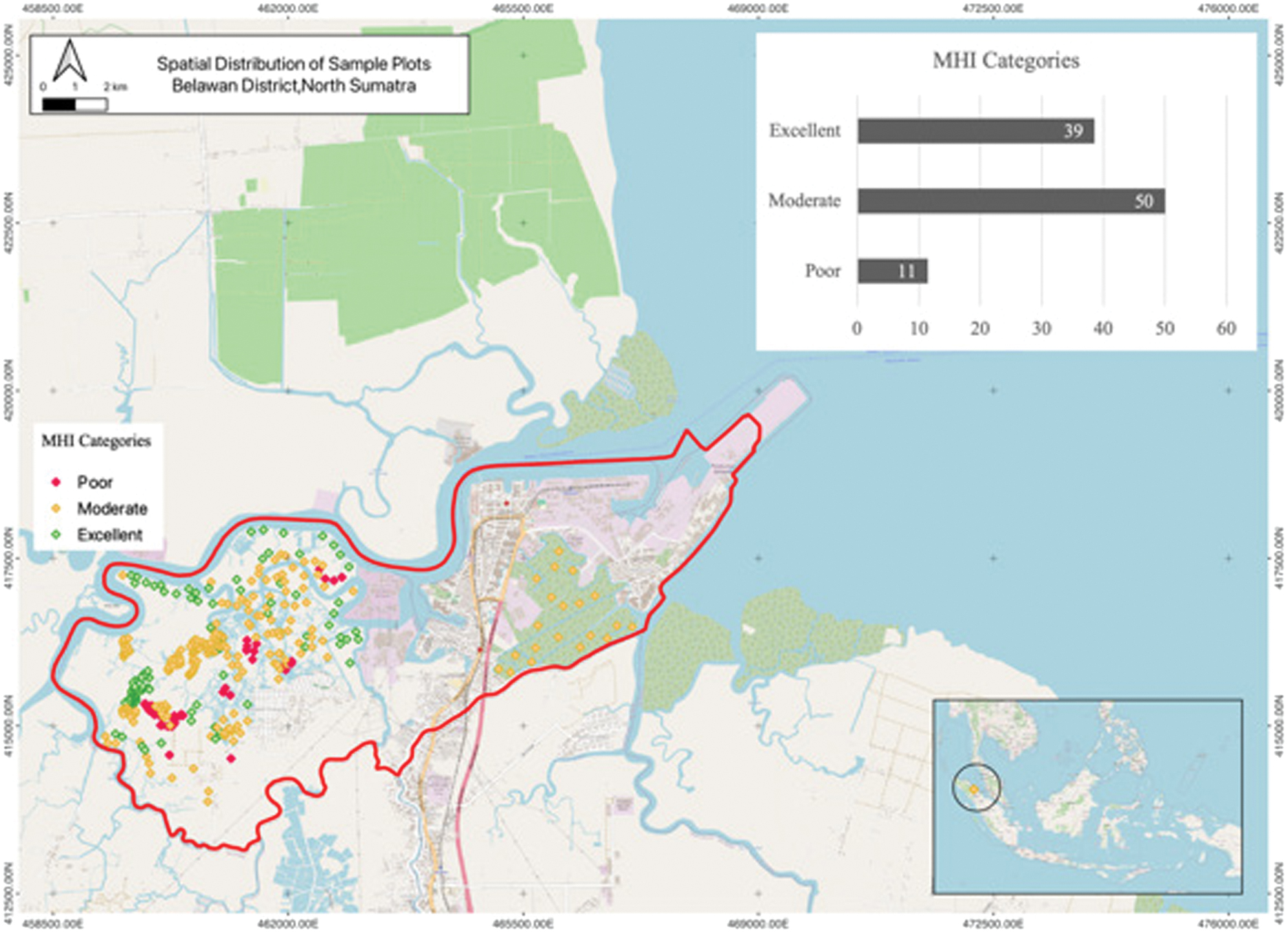 Fig. 4. Spatial distribution of sample plots and MHI calculations based on categories.
B.MODELING RESULTS AND VALIDATION
The MHI is estimated using three ML regression techniques: SVR, RFR, and K-nearest neighbor regression (KNN-R). Ground-truth measurements from 218 field plots serve as reference data, with MHI values calculated using Equation 1 as presented in Table I. Prior to modeling, all predictor variables are standardized through centering and scaling.
Table I. Reference and predictors data
| Plot | Reference data | Predictors | |||||||
|---|---|---|---|---|---|---|---|---|---|
| Sc | Sd | Snsp | MHI | NDVI | NBR | EVI | ARVI | mRE-SR | |
| 1 | 3.20 | 10.00 | 4.14 | 57.79 | 0.77 | 0.34 | 0.37 | 0.62 | 0.49 |
| 2 | 7.19 | 10.00 | 4.12 | 71.05 | 0.83 | 0.44 | 0.49 | 0.71 | 0.52 |
| 3 | 9.45 | 9.77 | 4.14 | 77.88 | 0.83 | 0.42 | 0.49 | 0.71 | 0.53 |
| 4 | 8.98 | 9.63 | 4.18 | 75.98 | 0.85 | 0.46 | 0.54 | 0.74 | 0.55 |
| 5 | 8.90 | 9.59 | 4.16 | 75.51 | 0.84 | 0.46 | 0.52 | 0.73 | 0.55 |
| 6 | 8.99 | 9.59 | 4.16 | 75.79 | 0.78 | 0.38 | 0.43 | 0.63 | 0.51 |
| 7 | 8.98 | 9.59 | 4.16 | 75.80 | 0.87 | 0.48 | 0.66 | 0.78 | 0.55 |
| 8 | 9.24 | 9.59 | 4.16 | 76.60 | 0.84 | 0.46 | 0.50 | 0.73 | 0.56 |
| 9 | 8.56 | 9.56 | 4.16 | 74.26 | 0.83 | 0.47 | 0.48 | 0.71 | 0.52 |
| 10 | 8.98 | 9.55 | 4.15 | 75.60 | 0.86 | 0.47 | 0.51 | 0.75 | 0.56 |
| 11 | 8.62 | 9.52 | 4.15 | 74.27 | 0.82 | 0.43 | 0.50 | 0.70 | 0.51 |
| 12 | 8.90 | 9.52 | 4.15 | 75.26 | 0.84 | 0.47 | 0.52 | 0.73 | 0.54 |
| 13 | 9.23 | 9.50 | 4.15 | 76.28 | 0.85 | 0.53 | 0.51 | 0.73 | 0.57 |
| 14 | 8.88 | 9.49 | 4.15 | 75.08 | 0.84 | 0.45 | 0.52 | 0.73 | 0.55 |
| 15 | 8.91 | 9.48 | 4.16 | 75.17 | 0.86 | 0.49 | 0.51 | 0.75 | 0.58 |
| 16 | 8.94 | 9.47 | 4.15 | 75.19 | 0.85 | 0.48 | 0.52 | 0.73 | 0.55 |
| 17 | 8.91 | 9.45 | 4.15 | 75.03 | 0.85 | 0.46 | 0.53 | 0.73 | 0.54 |
| 18 | 8.97 | 9.39 | 4.16 | 75.06 | 0.87 | 0.39 | 0.67 | 0.76 | 0.53 |
| 19 | 9.02 | 9.39 | 4.15 | 75.16 | 0.84 | 0.43 | 0.49 | 0.72 | 0.54 |
| 20 | 9.23 | 9.39 | 4.15 | 75.88 | 0.84 | 0.44 | 0.50 | 0.73 | 0.55 |
| 21 | 8.98 | 9.38 | 4.15 | 75.05 | 0.83 | 0.42 | 0.47 | 0.70 | 0.53 |
| 22 | 9.09 | 9.38 | 4.16 | 75.44 | 0.83 | 0.48 | 0.51 | 0.70 | 0.52 |
| 23 | 9.07 | 9.37 | 4.14 | 75.28 | 0.84 | 0.46 | 0.49 | 0.73 | 0.53 |
| 24 | 8.85 | 9.34 | 4.15 | 74.45 | 0.86 | 0.47 | 0.51 | 0.75 | 0.56 |
| 25 | 9.05 | 9.33 | 4.15 | 75.08 | 0.81 | 0.36 | 0.46 | 0.68 | 0.45 |
| Average | 6.19 | 7.47 | 4.13 | 59.31 | 0.78 | 0.40 | 0.44 | 0.64 | 0.48 |
Each model was trained and evaluated using 5-fold cross-validation, where the dataset is partitioned into five subsets and each subset serves once as the testing fold while the remaining four are used for training. Model performance is assessed using RMSE, MAE, and R2.
1).COMPARISON OF THREE ML ALGORITHMS
This study compares three ML regression approaches—SVR, RFR, and KNN-R—to predict MHI values. K-fold cross-validation with K set to 5 is utilized to assess model performance on the complete dataset. The outcomes of this comparison are illustrated in Fig. 5. The RFR algorithm was selected for MHI estimation due to its relatively superior performance, as indicated by lower RMSE and MAE values compared to SVR and KNN-R. Figure 5 shows that the RFR model demonstrates strong predictive performance in estimating MHI, as indicated by RMSE = 6.00, MAE = 4.73, and R2 = 0.82. This model is subsequently applied to the study area using the spectral index predictors presented in Fig. 6, including NBR, ARVI, NDVI, EVI, and mRe-SR.
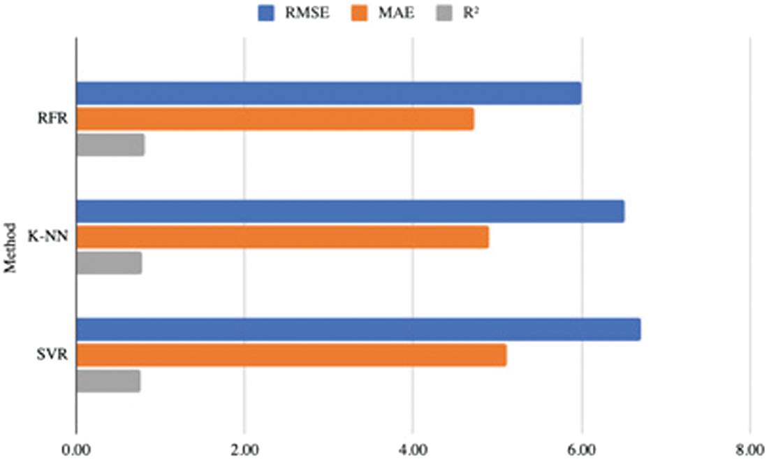 Fig. 5. Performance comparison of SVR, RFR, and k-NN models.
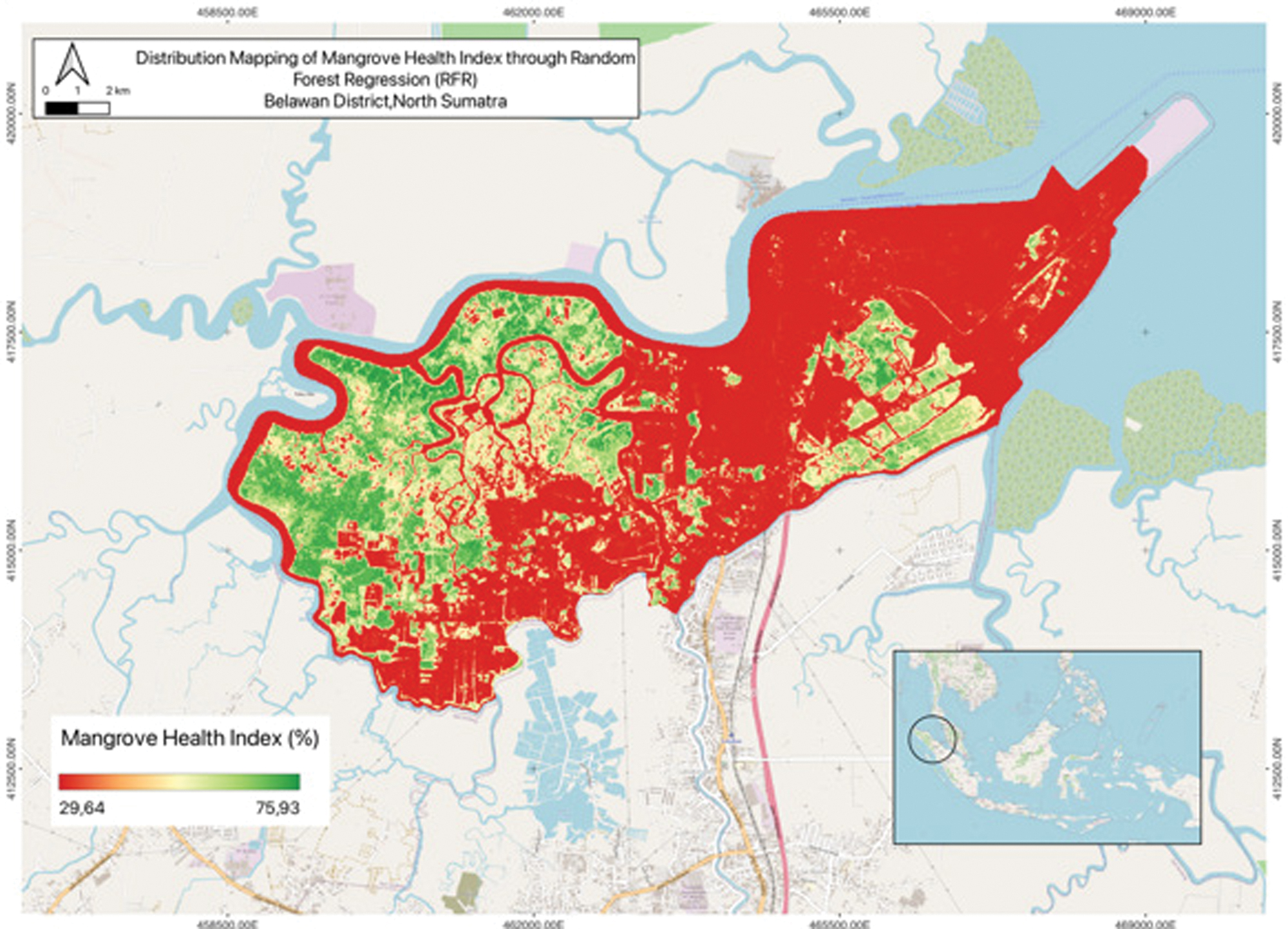 Fig. 6. Spatial distribution map of MHI in Belawan District.
Figure 6 demonstrates that MHI values range from 29.64 to 75.93 across the study area. This variation indicates that the health of the assessed mangroves covers a wide range, from poor to excellent. Approximately 698.63 ha, or 59.91% of the total area, is determined to be in moderate health condition based on the spatial distribution of the MHI. Areas classified as excellent and poor condition represent approximately 28.99% and 11.11% of the total area, respectively (Fig. 7).
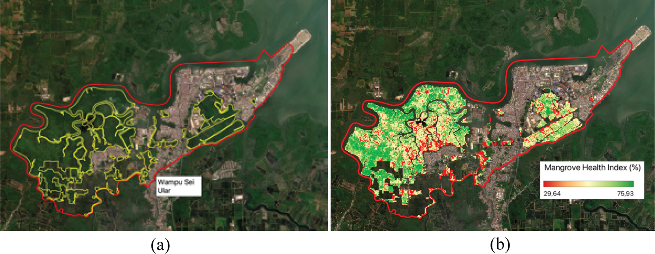 Fig. 7. Detailed visualization of mangrove-specific health conditions in Belawan District: a) mangrove area classification delineated with yellow boundaries and (b) spatial distribution of the Mangrove Health Index (MHI) within mangrove areas only.
IV.DISCUSSION
The findings of this study confirm the effectiveness of integrating remote sensing data with ML techniques in accurately assessing mangrove ecosystem health. The RFR model achieves strong predictive performance, as indicated by statistical metrics such as RMSE = 6.00, MAE = 4.73, and R2 = 0.82. These results suggest that the combination of spectral indices derived from Sentinel-2 imagery and robust regression algorithms provides a reliable and scalable approach for evaluating mangrove conditions. This outcome aligns with prior research that employed similar techniques for vegetation monitoring, where the RF algorithm demonstrated superior accuracy and model stability compared to other regression methods [13]. Previous studies applying remote sensing and ML techniques for mangrove health assessment have reported high classification accuracy and kappa coefficients of up to 97% and 0.94, respectively. Besides, the use of remote sensing indices, including NBR, ARVI [14], NDVI [12], EVI, and mRe-SR plays a key role in enhancing prediction accuracy. Their spectral sensitivity allowed differentiation between healthy and degraded mangrove stands, consistent with findings from [11,12], who demonstrated that combined spectral indices substantially enhance model robustness for mangrove and forest health estimation.
Moreover, ML can be applied to monitor and analyze changes in the mangrove ecosystem as time progresses. Several studies have demonstrated that the utilization of ML methods, such as RF and SVM, can provide highly accurate mappings of mangrove ecosystems. Furthermore, the utilization of satellite imagery data from sources such as Landsat-8, Sentinel-2, and WorldView-2 can be effectively used to monitor temporal changes in mangrove ecosystems. Therefore, ML serves as an essential tool for enhancing the efficiency of mangrove ecosystem monitoring and management [12,32,33].
An important advantage of this approach is its scalability. Remote sensing enables rapid assessment across large areas, which would be difficult and costly using traditional field surveys [9,11,34]. This is particularly valuable for regions with extensive but fragmented mangrove coverage, such as Belawan District.
However, certain limitations were identified in this study. The reliance on single-date imagery may restrict the ability to capture phenological and seasonal variations in mangrove health. The selected acquisition date does not explicitly account for tidal conditions, which may introduce variability in spectral values extracted from intertidal mangrove areas. Additionally, the RFR model requires validation across diverse ecological and climatic contexts to confirm its broader robustness. Other potential sources of uncertainty include atmospheric noise and varying spatial resolutions of satellite data. Future studies could address these limitations by incorporating multi-seasonal imagery, ground-based biophysical parameters, and advanced deep learning models such as convolutional neural networks (CNNs) or graph-based architectures. These methods have recently shown promise in capturing spatial heterogeneity and complex nonlinear relationships within ecological systems [35].
V.CONCLUSIONS
This study confirmed that RFR outperformed SVR and k-NN in predicting the MHI, achieving a high level of accuracy (R2 = 0.82) as validated by ground-truth measurements and K-fold cross-validation. The RFR model demonstrated superior capability in estimating critical ecological parameters, including canopy cover, stem diameter, and sapling density derived from Sentinel-2 spectral indices. The findings highlighted the effectiveness of combining medium-resolution satellite data with ensemble ML algorithms to produce reliable and scalable assessments of mangrove ecosystem health.
The integration of remote sensing and ML provided a transformative framework for continuous and spatially extensive environmental monitoring. Such an approach enabled rapid, cost-efficient evaluation of mangrove condition across broad coastal landscapes where field-based assessments are often limited. The results from this study underscored the potential of data-driven methodologies to inform restoration planning, biodiversity conservation, and blue carbon management initiatives.
Future research should emphasize the use of multi-seasonal or multi-year datasets to capture temporal variations in mangrove dynamics under changing climatic and anthropogenic pressures. Furthermore, incorporating socio-environmental variables such as land-use intensity, hydrological connectivity, and local management practices could enhance model interpretability and policy relevance. Advancing toward deep learning architectures, particularly convolutional and hybrid neural networks, also holds promise for improving predictive accuracy and generalizability. Collectively, these advancements can establish a more holistic, adaptive framework for monitoring and conserving mangrove ecosystems in the face of global environmental change.