JAIT

I.INTRODUCTION

The availability of cloud computing, big data analysis and machine-learning techniques allows big biology datasets to be explored and analyzed [1]. Microarray contains a large matrix of information and is being widely used by biologists and bio data scientists for monitoring the combinations of genes in different organisms. There is a kind of gene microarray data matrix called sequential gene microarray data matrix. This kind of data is a time series, as there are time factors in the data. The value of the data matrix of sequential gene microarray is obtained by testing gene expression at different time, which reveals the expression value varies with time [2]. The sequential gene microarray data always provides knowledge about the co-regulation of physiological processes and can reflect the relationship between biological processes and time. Therefore, the sequential gene microarray data plays an important role in the analysis of gene regulatory networks and dynamic biological processes [3 –5].

Time-series gene microarray data are generally stored in matrices, for a matrix D, each row in the matrix refers to one gene, while each column refers to the time setting of the experiment [6,7]. The value of the row is expressed as the expression level of the corresponding gene in the corresponding time.

Many biclustering models mine biclusters which are not continuous adjacent time, and thus these biclustering models cannot deal with time series data very well [8,9]. A contiguous column coherent (CCC) biclustering model was proposed by Sara C. Madeira et al. [10], which confined the pattern to continuous columns and was used to find all maximal contiguous column coherent biclusters. Considering the noise factor, Sara C. Madeira et al. improved the original CCC biclustering algorithm and proposed the e-CCC biclustering algorithm [11]. The experimental results showed that the e-CCC algorithm had better robustness to noise, and the biological information of the double clustering was enriched.

The important characteristics of a sequence are taken into account by CCC and e-CCC algorithms, which pay attention to the changing trend between two adjacent time points and the relative gene expression values rather than absolute values, and thus the model has strong anti-noise ability. However, CCC and e-CCC algorithm are all based on suffix tree string processing techniques, which have high spatial complexity and are difficult to deal with large-scale data. Moreover, these methods only qualitatively analyze the similarity degree of time series data, but do not give a quantitative method to calculate the similarity degree of time series, and thus it is difficult to quantitatively measure the similarity degree of two time series [12]. Without a measure of time series similarity, it is difficult to make further mathematical deduction and analysis of time series. Therefore, combining the core idea of contiguous columns coherent biclusters, it is critical and important to provide a measure of the similarity of time series.

The longest common subsequence (LCS) [13,14] is one of the classical similarity measures. However, LCS cannot contain all the information shared between two sequences. In order to capture more information between two sequences, Wang Hui [15] considered all subsequence factors of two sequences and proposed a new similarity measure, the number of all common subsequences (ACS), which obtained similarity by using dynamic programming strategy in polynomial time. However, the time series data contained sequential time sequence and had sequential relationship in continuous time. Both LCS and ACS did not take the adjacent time into account, and thus the similarity of this kind of data could not be properly measured. Considering the continuous time, it is more meaningful to pay attention to the same regular change in continuous time rather than the specific expression value. A uniform evolution type in continuous columns was proposed by Sara C. Madeira et al. [16]. CCC considered the same ascending and descending trend of the adjacent time points and the local longest mode. However, it lost the information of uniformly evolving pattern in the second, the third longer continuous columns, etc. In addition, this method only qualitatively analyzed the similarity degree of time series data. It did not quantitatively calculate the similarity of time series. It did not clearly propose or define a similarity metric to measure the similarity of two time series.

In order to measure the similarity of two sequential gene microarray series, a similarity measure, the number of coherent patterns in all continuous columns, is defined in this paper by considering the characteristics of time series. The expression of continuous time has time information factors and uses all common information between sequences, which can reflect the characteristics of uniform evolution in continuous time series. The simulation experimental results also show that the similarity measure is more accurate than other similarity measures, such as Euclidean distance and cosine distance.

Aiming at the problem of bicluster mining, combined with the characteristics of similarity measure proposed, we define a bicluster evaluation function for all continuous columns coherent biclusters to ensure the consistency of biclusters and implement an efficient algorithm to apply the evaluation function to specific bicluster mining. The results also show that the bicluster algorithm proposed in this paper can find significant results of biological knowledge from the sequential gene microarray data.

The remainder of this paper is as following. Section II explains the All Contiguous Coherent Columns (ACCC) similarity measure. Section III presents our proposed BicACCC method and algorithm. Section IV outlines the datasets and experiment design. Section V discusses the simulation experimental results. Finally, section VI draws conclusions.

II.ALL CONTIGUOUS COHERENT COLUMNS SIMILARITY

The idea of calculating ACCC in given continuous columns of the same length is as follows. Given two rows to be computed, count the number of patterns with the same trend in two rows in any continuous columns. The number obtained is the ACCC similarity.

The similarity in all continuous columns focuses on the common evolutionary rules of data in continuous time. First, the original sequence (whose number of elements is n) is preprocessed and transformed into the differential sequence (whose number of elements is n−1) [17]. The value in d sequence reflects the rising and falling trend from the time to the next time. In this paper, we divide the trend into two cases: rising and non-rising. The way in which the original sequence is preprocessed into a differential sequence is shown as the following:

d_{i} = {\begin{cases} 1, & if a_{i + 1} - a_{i} > 0 \\ 0, & if a_{i + 1} - a_{i} \leq 0 \end{cases}

(1)

Where a_i+1 and a_i is the (i + 1)^th and the i^th element in the sequence a respectively.

Firstly, the original sequence is preprocessed, and the original sequence is transformed into the differential sequence. For convenience, the preprocessing process is expressed as d = Difference(a): The calculation of the differential sequence is as follows:

Difference (a) = {\begin{matrix} 1, & if a_{i + 1} - a_{i} > 0 \\ 0, & if a_{i + 1} - a_{i} \leq 0 \end{matrix} i = 1, 2, \dots, | a | - 1

(2)

The original data are inspected and the differential sequence is obtained by preprocessing. By calculating the changing trend of two successive elements in the original data, where the rising is 1, and the non-rising is 0. Thus, a sequence with 1 element shorter than the original data can be obtained, which is called the differential sequence.

After this preprocessing, the original matrix is transformed into the differential matrix. Considering two rows of time series data, we focus on the number of patterns with the same trend in the adjacent time points. The bigger the number of the continuous columns coherent patterns in two time series is, the more similar they are.

$A C C C (a, b)$ refers to the similarity of the sequence $a$ and $b$ . The calculation is as follows. The sequence $a$ and $b$ are different rows in the difference matrix.

Two difference sequences after being preprocessed are investigated, and the similarity is obtained. Two differential sequences are operated on Inclusive-OR operation, that is, in the same columns, if the Boolean values are the same, then the result is 1, and vice versa, it is 0. Thus, the similarity sequence is obtained, which has the same length as the differential sequences.

Consider the similarity sequence and calculate the similarity. The number of segments appearing in all 1, and the number of 1 in each segment are counted. Finally, the number of continuous columns coherent patterns, namely similarity ACCC, is calculated by the equation (3).

ACCC (a, b) = \sum_{i = 1}^{sects} \frac{n_{i} (n_{i} + 1)}{2}

(3)

Where sects is the segments appearing in all 1 in the similarity sequence obtained by OR operation from the deferential sequences a and b, and n_i is the number of 1 in the i^th segment. Figure 1 shows the pseudo code for calculating ACCC.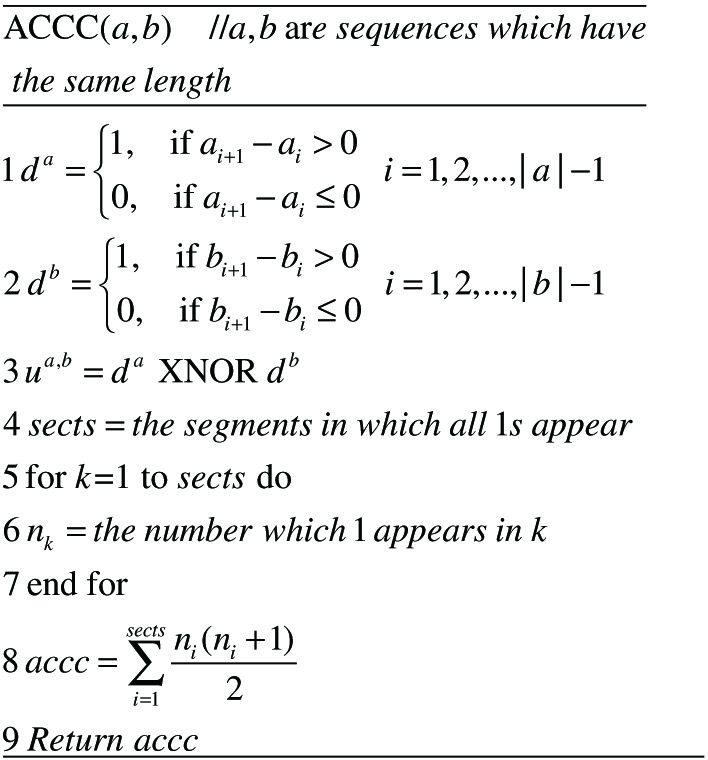

Fig. 1. The pseudo code for calculating ACCC.

For example:

Given a similarity sequence (1,1,0,0,1,1,1,0,1), it has 3 segments of all 1. Each segment is underscored as (1,1,0,0,1,1,1,0,1), thus the number of 1 in each segment is: n₁ = 2, n₂ = 3, n₃ = 1. Then the similarity is: accc = 3+6+1=10.

Given the original sequences as:

a = (2, 8, 7, 5, 7, 9), b = (3, 5, 8, 6, 3, 7), c = (6, 5, 9, 7, 5, 2)

The process of obtaining the differential sequence is as follows.

For example: Obtain the differential sequence from the sequence a. It is show in the sequence a that the first element is 2 and the second is 8. As 8 is greater than 2, then the first element in the sequence d^a is 1, and so on. The last group is 9 > 7, so the last element of d^b is 1. Thus, we obtain the sequence d^a = (1,0,0,1,1).

The obtained differential sequences are:

d^{a} = (1, 0, 0, 1, 1), d^{b} = (1, 1, 0, 0, 1), d^{c} = (0, 1, 0, 0, 0) .

The process to obtain the similarity sequence:

To obtain the similarity sequence u^a,b from the sequence a and the sequence b, where d^a = (1,0,0,1,1), d^b = (1,1,0,0,1). The first elements in both d^a and d^b are 1. The result of inclusive-OR operation of (1,1) is 1. Thus, the first element of the sequence u^a,b is 1. The same procedure is repeated and is obtained.

The other similarity sequences are:

u^{a, b} = (1, 0, 1, 0, 1), u^{a, c} = (0, 0, 1, 0, 0), u^{b, c} = (0, 1, 1, 1, 0) .

To calculate the similarity:

Obtain the similarity of the sequence b and the sequence c from, u^b,c = (0,1,1,1,0) where the series (1,1,1) represents the changes in the differential sequences (1,0,0) (rising, falling, falling), which includes the following contiguous columns coherent patterns (i->j: y, the trend from the column i to the columns j is y, where y = 1 represents rising and y = 0 represents falling):

2->3:1
3->4:0
4->5:0
2->3->4:10
3->4->5:00
2->3->4->5:100

There are six contiguous columns coherent patterns, and thus the similarity is 6.

ACCC (a, b) = 3, ACCC (a, c) = 1, ACCC (b, c) = 6 .

III.BicACCC BICLUSTERING ALGORITHM

We propose a biclustering based on ACCC.

A.THE EVALUATION OF A BICLUSTER

The following is the description of the relative definitions.

(1)C represents the continuous columns and C^j,k represents the continuous columns from the jth column to the (j + k−1)^th column.
(2)S represents the core of the bicluster and S^j,k represents the series belong to C^j,k.
(3)R represents the supporting row set. If a row has a pattern in the given continuous columns, it is said that this row supports the pattern. The supporting row set refer to the row set that support a bicluster core. R^j,k means the supporting row set of C^j,k.
(4)The subscript represents the serial number of the bicluster. The ith bicluster core is S^j,k whose continuous columns is $C_{i}^{j, k}$ and the supporting row set is $R_{i}^{j, k}$ .

Firstly, a bicluster measure method is defined, which employs the information in all continuous columns coherent patterns that is the number of all continuous columns coherent patterns per column (abbreviated as perACCC).

The procedure of biclustering method based on all continuous columns coherent patterns is to calculate the number of all continuous columns coherent patterns of each row and the core of bicluster, then sum these numbers, and divide the sum result by the number of columns in the bicluster, so as to get the value to measure the bicluster [18].

The evaluation of a bicluster is stated as the following:

perACCC (I, J) = \frac{1}{| I | | J |} \sum_{i \in I} ACCC (a_{i J}, a_{I J})

(4)

Where I is the supporting row set of the bicluster, J is the continuous columns set of the bicluster, a_iJ the sequence of the i_th row under the continuous columns J, a_IJ is the core bicluster. ACCC(a_iJ,a_IJ) refers to the similarity value of the sequence a_iJ and a_IJ. If the core bicluster is

S_{i}^{j, k}

, the row set is

R_{i}^{j, k}

and the column set is

C_{i}^{j, k}

, then the corresponding relation of the formula is

I = R_{i}^{j, k}

J = C_{i}^{j, k}

a_{I J} = S_{i}^{j, k}

A C C C (a_{i J}, a_{I J})

represents the similarity between the sequence a_i and S_i under the continuous columns.

According to the definition of ACCC similarity, it can be expanded as follows:

ACCC (a_{i J}, a_{I J}) = \sum_{k = 1}^{{sects}^{J}} \frac{n_{k} (n_{k} + 1)}{2}

(5)

Where sect^J represents the number of all 1 s in the continuous columns, n_k is the number of 1 in the k_th segment.

From (4) and (5), we can obtain (6) :

perACCC (I, J) = \frac{1}{| I | | J |} \sum_{i \in I} \sum_{k = 1}^{{sects}^{J}} \frac{n_{k} (n_{k} + 1)}{2}

(6)

Given a matrix D = (R,C),where R is the row set and C is the column set, is a submatrix in D, where R_s and C_s are the subsets of R,C respectively. If C_s is the continuous columns, and the submatrix S = (R_S,C_S) has larger perACCC, then S = (R_S,C_S) is a bicluster of all contiguous columns coherent patterns in D = (R,C), abbreviated as BicACCC.

B.THE ALGORITHM OF BicACCC

The framework of BicACCC is shown as Figure 2:

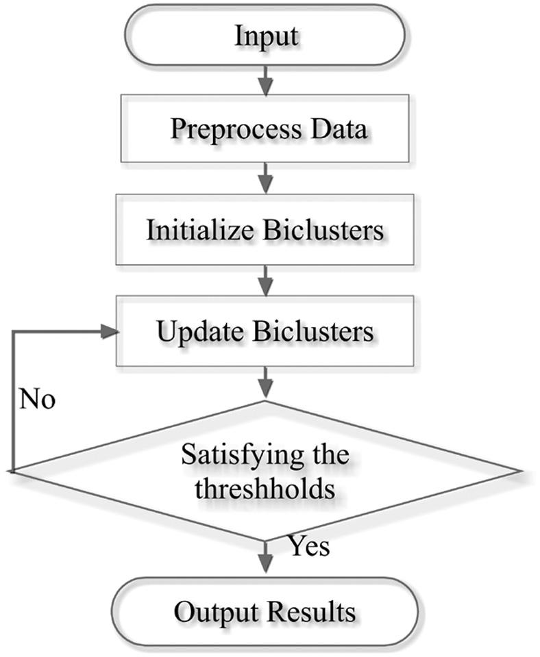Fig. 2. The framework of BicACCC.

The steps of BicACCC algorithm:

(1)Data preprocessing: Generate the differential matrix by transforming the original matrix into a matrix which implies the trend of any two adjacent time points.
(2)Initialize biclusters: Firstly, select the core of bicluster, that is, to select randomly the combination of several pairs of rows and consecutive columns in the data matrix to get the core bicluster. Secondly, initialize the row set of the bicluster, that is, to calculate the perACCC value of each row and each core in the data matrix, select the row with the largest value for the core and apply the row to the row set of the core. The third step is to update the core of the bicluster, that is to say, to calculate the mode of each column to the row set in the bicluster and use the number of the mode as the value of the corresponding column of bicluster, so as to get the updated core of the bicluster. The complete algorithm is given in Figure 3.
(3)Update biclusters: Firstly, calculate the perACCC value of the bicluster before updating; Secondly, update columns by adding and deleting; the third step is to update rows by adding qualified rows through scanning the data matrix; and the fourth step is to update the core bicluster by mode method; The fifth step is to calculate the perACCC value of the bicluster after updating; the sixth step is to calculate the change rate of the perACCC value of the bicluster before and after updating, and to determine whether the preset threshold is satisfied, so as to determine whether to continue updating the bicluster iteratively.
(4)Output results: setting a set of the row and column thresholds, deleting the bicluster which does not meet the preset row and column thresholds, and obtaining the bicluster which satisfies the row and column thresholds.

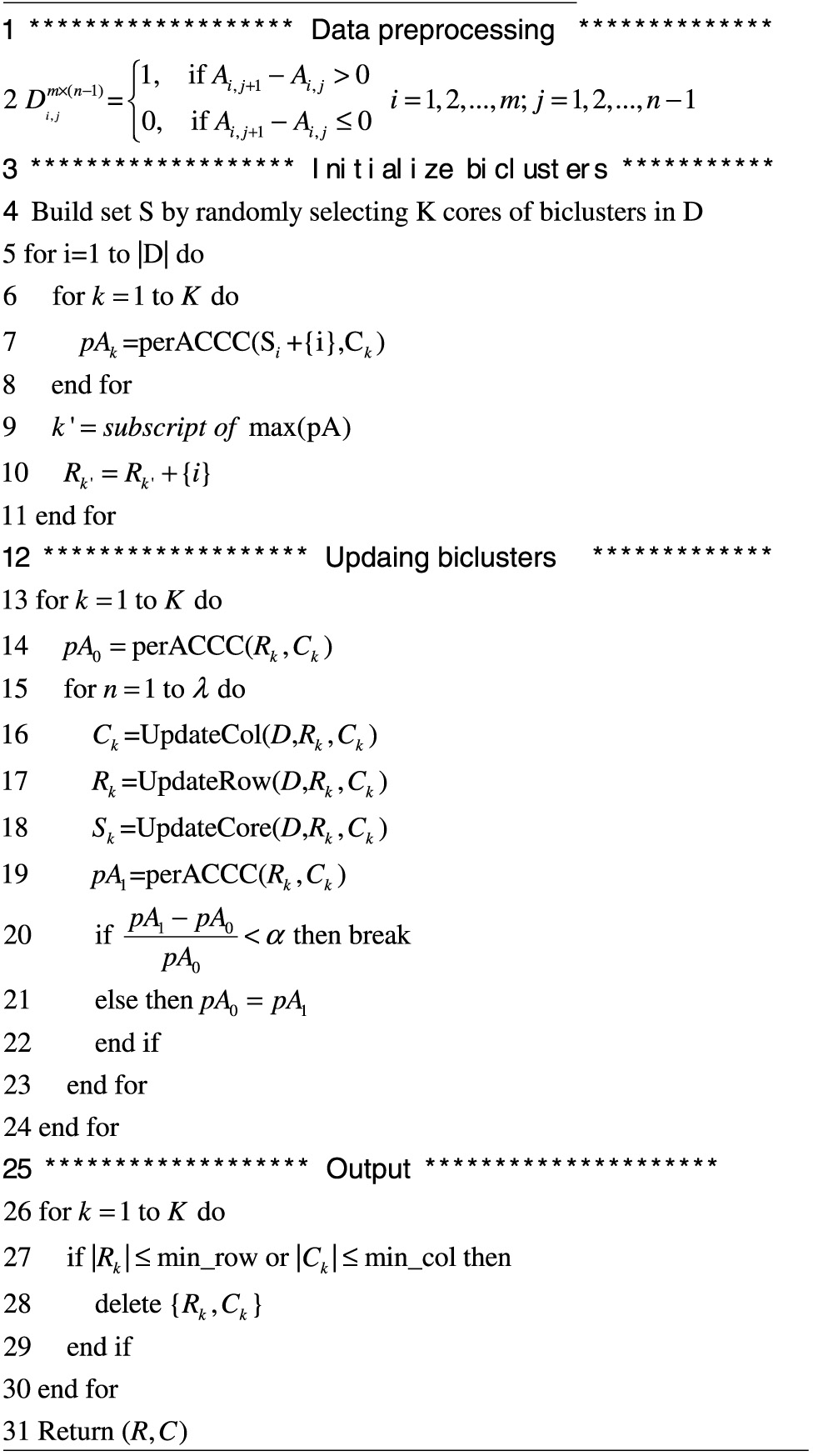Fig. 3. The pseudo code of BicACCC.

C.EXAMPLE OF THE ALGORITHM

The sequential gene microarray data matrix is time series data whose value is obtained by testing gene expression at the different time. The value in the matrix reveals that the expression value varies with time 0. This paper focuses on the consistent evolution of data over time rather than on the specific value of gene expression. The model studied in this paper does not consider the actual expression value of the gene at the time point, but it considers the variation trend of the gene at the adjacent time points.

1)Preprocessing

There are many rules of change, which can be divided into three types: rising, unchanged and falling. They can also be divided into five types: sharp rise, slow rise, basically unchanged, slow decline and sharp decline. In this paper, we focus on the uniform evolution in continuous columns, and define the change as two cases, i. e. rising or non-rising. Therefore, in the process of data preprocessing, the original data matrix A^m×n is transformed into the differential matrix D^m×(n−1). In the original data matrix, a_ij is the element in i^th row and the j^th column in A. In the differential matrix, d_ij is the element in the i^th row and the j^th column which represents the upward and downward trend from a_i,j to a_i,j+1 in the original data matrix A. The upward and non-upward trends are expressed by 1 and 0 respectively, i.e. if a_i,j+1−a_i,j>0 then, d_ij = 1; if a_i,j+1−a_i,j≤0 then d_ij = 0. The differential matrix obtained by the above method is a matrix of m×(n−1) whose values are only 0 and 1. The operation of each row of the original matrix is the same as the method of obtaining the difference sequence described in the ACCC similarity described above. The specific calculation method is shown in equation 2.

The original data matrix is shown as Table 1, and the differential data matrix transformed by preprocessing for Table 1 is shown as Table 2. For instance, in the first row of Table 1, the expression values at time t1 and t2 are 0.55 and 0.19 respectively, because 0.19 < 0.55, the first column’s value of the row in the difference matrix is 0. Similarly, when the original data in row α is 0.83 > 0.19, so the second column’s value of the row α is 1. With this preprocessing method, the original data matrix represented in Table 1 can be transformed into the differential data matrix represented in Table 2.

Table I The original time series gene data

Gene Time	t1	t2	t3	t4	t5	t6
a	0.55	0.19	0.83	0.48	0.76	0.38
b	0.78	0.42	0.27	0.56	0.69	0.32
c	0.54	0.88	0.76	0.69	0.41	0.64
d	0.16	0.34	0.4	0.52	0.81	0.25

Table II The differential matrix

Row Column	1	2	3	4	5
a	0	1	0	1	0
b	0	0	1	1	0
c	1	0	0	0	1
d	1	1	1	1	0

2)Initialize biclusters

The procedure for initializing biclusters are described below.

Select a bicluster core.

In the data matrix, several pairs of rows and consecutive columns are randomly selected to obtain a bicluster core. The method of randomly selecting K cores of biclusters is to randomly select a row in the data matrix as the core row, and then randomly select a continuous column. The expression pattern of the selected row on the selected continuous columns constitutes the core of the bicluster. In fact, this step chooses the initial column set of the bicluster. For convenience, it is marked as the ith bicluster’s core $S_{i}^{j, k}$ , in which the core row is represented as and the continuous columns is represented as $C_{i}^{j, k}$ .

As shown in Figure 4, in the differential matrix of Table 2, it is advisable to set the number of bicluster cores as 2, that is, K = 2. Randomly select two bicluster cores, the first core S₁ is the row b = [0 0 1 1 0], which has continuous columns (the second column and the third column). The second core S₂ is the row a = [0 1 0 1 0], which are listed consecutively in the column 1 and the column 2. As shown in Figs. 2, and 3, the numbers in the box represent column labels, and the lists in the dotted box represent continuous columns. The cores are S₁ = (ce = [0 0 1 1 0], C = {2,3}), S₂ = (ce = [0 1 0 1 0], C = {1,2}) respectively.

3)Initialize the row set of the bicluster

The row set refers to the set of supporting rows that support corresponding bicluster cores. The procedure is stated as follows: calculate the perACCC values of each row and all cores, select the core with the highest perACCC values, and add the row to the supporting row set with the highest perACCC values, remark it as the ith supporting row set $R_{i}^{j, k}$ . As the continuous columns $C_{i}^{j, k}$ are selected in previous step, so the bicluster is expressed as $(R_{i}^{j, k}, C_{i}^{j, k})$ .

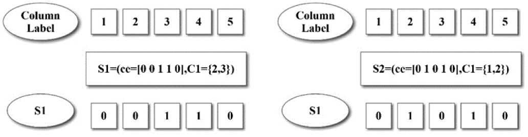Fig. 4. An example of selecting the core of biclusters.

As shown in the Figure 5, calculate the perACCC values of the row a with the core S₁ and S₂ respectively, then compare the results, because 0 < 1.5, so the row a is added to the corresponding row set R₂ in S₂. The next is to compute the perACCC values of the row b and the row c, and we get R₁ = {b,c}. As for the row d, since its perACCC values is 0.5 = 0.5, so it is added to the two cores and we get R₁ = {b,c,d}, R₂ = {a,d}. Finally, we get the initial row sets and the initial column sets, R₁ = {b,c,d}, C₁ = {2,3}, R₂ = {a,d}, C₂ = {1,2}.

4)Update the core of the bicluster

For each column of the differential matrix, calculate the mode of each column on the row set of the bicluster, and use the mode as the value of the corresponding column of the core of the bicluster, thus we obtain the updated core of the bicluster. If there are more than two modes, randomly select one of them to update. It should be noted that when updating the bicluster core, all columns should be updated, therefore it is convenient to update the column set later.

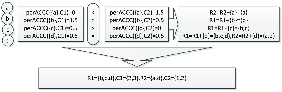Fig. 5. An example of initialize the row set of the bicluster.

As shown in the Figure 6, when the first bicluster is considered, and the row set and column set are R₁ = {b,c,d}, C₁ = {2,3}, respectively. The row values of b,c,d is in the upper right long box. Considering the first column, the number of 0 is 1, marked as # 0 = 1, and the number of 1 is 2, marked as # 1 = 2, because # 0 < # 1, so the core of the first column is listed as 1, as shown in the row ce. Next, the process is repeated from the second column to the last column to get the core row ce = [1 0 1 1 0]. Thus the core is updated as S₁ = (ce = [1 0 1 1 0], C = {2,3}). Considering the second bicluster, the method is similar, the core are obtained as S₂ = (ce = [1 1 0 1 0], C = {1,2}).

5)Update biclusters

The procedure for updating biclusters are described below.

Step 1: Calculate the perACCC value of the bicluster before updating.The method of calculating perACCC value of biclusters is introduced in the overview of algorithm as shown in equation 4.Example: Initialize biclusters, Take the first bicluster as an example whose row set is R₁ = {b,c,d} and the continuous columns is C₁ = {2,3}. The perACCC of is calculated as pA₀ = 0.83.
Step 2: Update columns by adding and deleting.

In order to adjust the continuous columns pattern of biclusters flexibly, the columns are updated by adding and deleting. The conditions for adding and deleting the continuous columns are as follows:

The Condition for adding columns: If a column is added and the calculated perACCC value increases, then the column can be added.

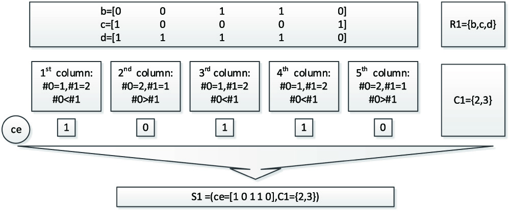Fig. 6. Updating the core of the bicluster.

The condition for deleting columns: If a column is deleted and the calculated perACCC value increases, then the column can be deleted.

The steps for adding and deleting contiguous columns are as follows:

First, add continuous columns to the right until the end of expansion, then continue to add continuous columns to the left until the end of expansion. Delete operations from the leftmost column to the right until stop. Then delete operations from the rightmost column to the left until stop. If continuous columns expand to the right, then you do not need to delete the column on the right because only the perACCC value increases in the process of expanding and adding columns is permitted. Similarly, if continuous columns expand to the left, you do not need to delete the column on the left. Only when no column has been added to the right expansion or the left expansion, then the column on the right or the left can be deleted, and thus it avoids unnecessary operations.

The pseudo code for updating the column set of biclusters is shown in Figure 7.

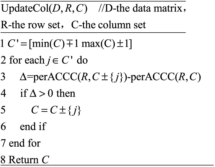Fig. 7. The pseudo code of updating the column set of biclusters.

An example of updating the column set of biclusters is shown in Figure 8.

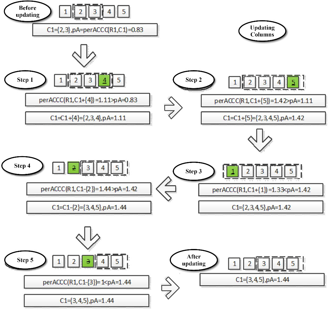Fig. 8. The example of updating the column set of biclusters.

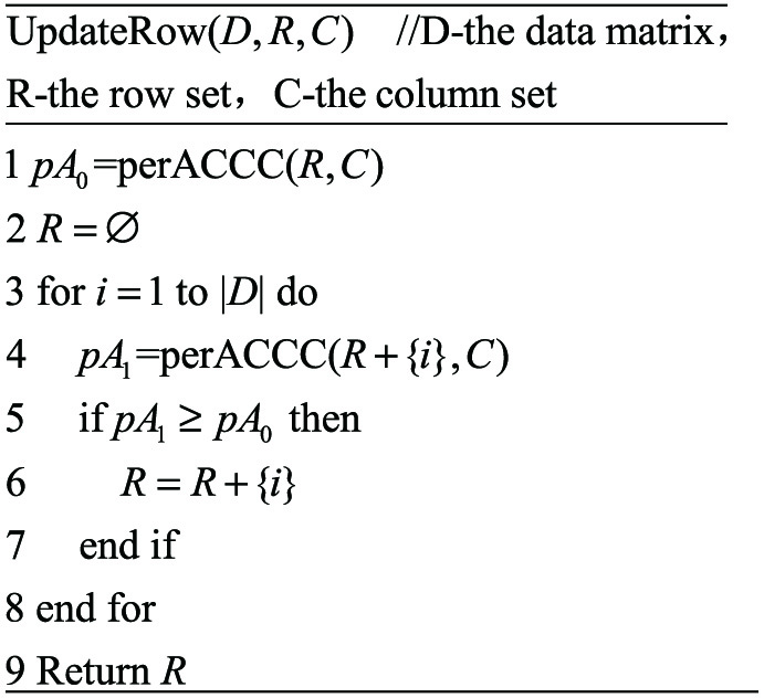Fig. 9. The pseudo code of updating the row set of biclusters.

Given the bicluster whose row set is R₁ = {b,c,d} and the continuous column set C₁ = {2,3}, calculate the perACCC value of the bicluster first, and mark it as pA = perACCC(R₁,C₁ as shown in the Figure 8. “before updating” pA = 0.83. Then add contiguous columns to the right. First, consider adding column 4 as shown in step 1 of the Figure 8, then the continuous columns are {2,3,4}. The perACCC value is calculated to be 1.11, because 1.11 > pA = 0.83, so it is confirmed to add column 4 to the continuous column and assign the new perACCC value 1.11 to pA. Continue to expand the contiguous column to the right and add the fifth column, as shown in step 2 of the Figure 8, which is the same as the previous step, thus the continuous columns are {2,3,4,5}. The perACCC value is calculated to be 1.42, because 1.42 > pA = 1.11. Thus, it is confirmed to add the fifth column to the contiguous columns and assign pA the new perACCC value 1.42. Because column 5 is the rightmost column, stop expanding to the right. After the right expansion stops, the left expansion begins. First, consider adding column 1, as shown in step 3 of the Figure 8, the continuous columns are {1,2,3,4,5}. Then calculate the perACCC value and get 1.33, because 1.33 < pA = 1.42, so do not add column 1 to the continuous columns, while maintaining the value of pA as 1.42. Because column 1 is the leftmost column, it can no longer be expanded to the left, therefore stop expanding to the left.

After the adding step is completed, we begin to delete the continuous columns. First, consider the column 2 as shown in step 4, when the column 2 is deleted, the perACCC value is calculated to be 1.44, because 1.44 > pA = 1.42. Thus, it is confirmed that the second column is deleted from the continuous column set and the new perACCC value (1.44) is assigned to. Continue to delete column 3, as shown in the step 5 of the Figure 8, and calculate the perACCC value as 1, because, 1 > pA = 1.44 hus we do not delete column 4 and maintain the value of pA as 1.44. Because the initialized continuous columns are {2,3}, after the column expansion it becomes {2,3,4,5}. That is to say, the column 4 and 5 are confirmed to be added to the continuous columns in the process of extending to the right, so the process of deleting columns from the right to the left is not necessary. Finally, the last continuous columns C₁ = {3,4,5} generated by this round of process is shown in ‘Updated’ of the figure.

Step 3: Update the row set by adding qualified rows by scanning the data matrix.

The conditions for adding rows are as follows:

If the calculated perACCC value after adding a row is greater than or equal to the perACCC value of the bicluster before adding the row, then confirm to add the row, otherwise do not add.

The updating steps are as follows:

First, the perACCC value of the biluster is calculated, then the data matrix is scanned once and the ACCC value between each row and the bicluster core is calculated. Then, the ACCC value is divided by the number of continuous columns in the bicluster core, and the row whose perACCC value is greater than or equal to the previous perACCC value is added to the row set.

In fact, the effect of scanning the matrix and updating the row sets is equivalent to deleting the rows whose perACCC value are smaller than the original bicluster’s perACCC value, and then adding rows whose perACCC values are greater than or equal to the original bicluster’s perACCC value. This method can add rows and delete rows at the same time.

An example of the process of updating the row set is shown in Figure 10.

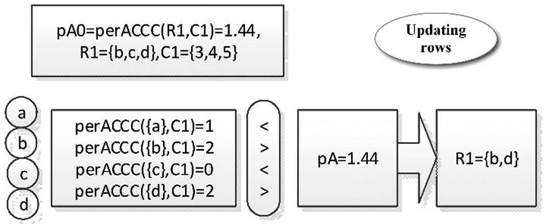Fig. 10. The example of updating the row set of biclusters.

The support row set obtained in the above steps are R₁ = {b,c,d}, and the continuous columns are C₁ = {3,4,5}. The bicluster core is S₁ = (ce = [1 0 1 1 0],C = {3,4,5}). The perACCC value after updating columns is pA = 1.44. Scanning all rows in the differential matrix, we first calculate the perACCC of the first row α(α(perACCC({a},C₁) = 1),), because 1 < pA = 1.44, so we do not add row b to the row set. The same process is done on the second row b (perACCC({b},C₁) = 2), because 2 > pA = 1.44, so add the row b to the row set. After scanning, the row set R₁ = {b,d} are obtained, compared with the original row set{b,c,d}, the row c is deleted because it is not satisfied the condition.

Step 4: Update the bicluster core by the mode method.The method of updating the bicluster core is the mode method, which has been described in the above. The pseudo-code is shown in the following Figure 11.The process of updating the bicluster core is shown as the following and the core S₁ = (ce = [1 0 1 1 0],C = {3,4,5}) is obtained.
Step 5: Calculate the perACCC value of the updated bicluster.Example: After updating the bicluster, the perACCC value of the bicluster is calculated as pA₁ = 2.
Step 6: Calculate the changing rate of perACCC before and after updating the bicluster.

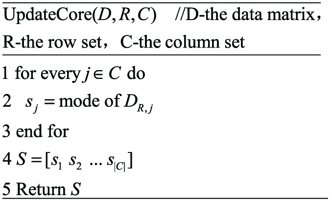Fig. 11. The pseudo code of updating the core of biclusters.

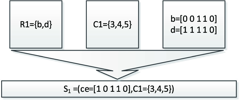Fig. 12. The example of updating the core of a bicluster.

The method to decide whether to continue iteration or not is to set a changing rate threshold α and the upper limit of iteration number γ. The perACCC value are calculated before the column and the core are updated as pA₀, and after updated it is pA₁. If the changing rate from pA₀ to pA₁ is less than the preset changing rate threshold α or the number of iterations reaches the upper limit γ., then stop iteratively updating the bicluster; otherwise continue updating iteratively. The calculation of the rate of changing and the judgment are as follows:

\frac{p A_{1} - p A_{0}}{p A_{0}} < α

(7)

Examples of iterations are shown in Figure 13.

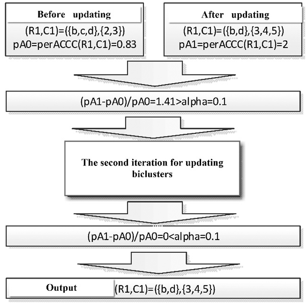Fig. 13. Calculating the changing ratio and the updating iterations.

In this example, it is possible to set the changing rate threshold α = 0.1, which means that the changing rate of the perACCC value needs to be less than 0.1 before the iteration stops. As shown in the Figure 13, the perACCC value of the bicluster before updated is pA₀ = 0.83. After the bicluster is updated, the perACCC value is pA₁ = 2. The changing rate is 1.41, because 1.41 > 0.1. In the second iteration, the perACCC value of the bicluster before updated is pA₀ = 2. After the bicluster is updated, the perACCC value is pA₁ = 2, and the change rate was 0. Because 0 < 0.1, the iteration is stopped and the row set of the bicluster are obtained.

6)Output

In order to avoid finding meaningless biclusters with too few rows or columns, a row threshold and a column threshold are set. Only the biclusters satisfying both the row threshold and the column threshold is meaningful. Therefore, we only output the bicluster satisfying the pre-determined row and column thresholds and delete those biclusters that do not meet the row and column thresholds.

The steps of output are as follows: Set a set of row and column thresholds, delete the bicluster if the bicluster does not meet the preset row and column thresholds, output the biclusters which satisfy the row and column thresholds.

In this example, we set the row threshold min_row = 2 and the column threshold min_col = 2.

After updating the biclusters, the row set and the column set of the first and the second bicluster are (R₁,C₁) = ({b,d},{3,4,5}), (R₁,C₁) = ({a},{2,3,4,5}) respectively. Obviously, the second bicluster has only one gene whose number of rows is 1 < min_row = 2, so it is deleted. Therefore, the final result is (R₁,C₁) =({b,d},{3,4,5})

IV.DATASETS AND SIMULATION EXPERIMENTS

Simulation study is conducted on synthetic data in order to evaluate the performance of the proposed algorithm. The relationship between the running time of the program and the size of the synthetic data set is analyzed, that is, the scalability of the algorithm, as well as the mining speed of single bicluster, are analyzed.

In order to analyze the biological correlation of the biclusters, the GOToolbox is used for analyzing the real gene microarray data [19,20]. Gene Ontology (GO) is often used to test the biological authenticity of clustering or biclustering results, that is, to reflect the biological significance of clustering or biclustering results. By focusing on the P-value of the biclustering results from GO and analyzing them from the statistical point of view, we can obtain the significance of the enrichment degree of the biclusters in biological function. Calculate the P-value of known gene types and the biclusters, and then count the ratio of the biclusters whose P-values are less than the pre-set P-value to the total number of biclusters. We thus get the statistical significance of the enrichment of the biclusters on biological processes. In order to illustrate the performance of the algorithm more comprehensively, several comparative experiments with other biclustering algorithms are carried out on the same synthetic data and the real gene microarray data, and the results of the proposed algorithm and other algorithms are simulated analyzed. In addition, the proposed similarity measure ACCC is applied to K-means algorithm for enrichment analysis in the gene microarray data. At the same time, Euclidean distance and cosine distance are applied to the same gene microarray data for enrichment analysis in K-means algorithm. The comparative experimental results show that ACCC can describe the similarity of time series data more accurately.

Simulation experiments based on synthetic data and the real gene microarray data sets are carried out to analyze the performance of the proposed algorithm and the biological significance. The real gene microarray data sets include three gene microarray data sets, yeast microarray data 0, mouse cell microarray data and human cell microarray data.

For synthetic data sets, the range of data is 0 to 1, and the data is uniformly distributed. One of the data sets has the same number of columns, which are 20. The number of rows starts at 1000 and ends at 2000 with the increasing step 100. Therefore, there are 11 data matrices. Another dataset has the same number of rows, which are 1000. The number of columns starts at 20 and ends at 40 with the increasing step 2. There are also 11 data matrices.

The real gene microarray data sets include three gene microarray data sets.

Yeast microarray dataset: Yeast microarray dataset is a sequential gene microarray data, which is tested by CHO et al. 0. CHO et al. [21] on 6178 genes and 17 sampling time points. The interval between two sampling time points was 10 minutes. In this data matrix, different rows refer to different genes, different columns refer to different experimental time points, and the values in the matrix refer to the expression level of the corresponding genes at the corresponding time points. Some of the missing values in this data set are filled with the ‘cubic spline interpolation method’ proposed by Troyanskaya et al. 0, and those rows with extremely large missing values are deleted. After processing the missing values, the size of the data matrix is 6147 × 17.

Rat microarray dataset: Rat microarray dataset is the traumatic brain injury data set of Salvia [22]. It is an analysis of the lateral cortex of the brain from Wistar males for up to 48 hours after traumatic brain injury (TBI). After preprocessing the data, the size of the data matrix is 8162 × 16.

Human cell microarray dataset: Human cell microarray dataset is used in hematopoietic stem cells to study CD34 + and is processed by uridine triphosphate. The data is processed in about 24 hours. The size of the original data matrix is 22283 × 6 which contains some duplicated data, i.e. several rows of time series experiments that record the same gene. After processing, only one row for a gene is retained in the matrix, and the size of the remaining data set is 5477 × 6. The data set can be found at ftp://ftp.ncbi.nlm.nih.gov.

V.RESULT ANALYSES

The platform used in the experiment is: Intel ® Pentium ® CPU G2030 @ 3 GHz 3 GHz; RAM: 8 G; working speed: 3 GHz; computer system: Windows 10; operating software: VS2010; experimental programming language: C++.

A.THE PERFORMANCE OF THE ALGORITHM THROUGH SIMULATION

Assume that matrix A(m,n) with m rows and n columns, if there are k biclusters in the matrix A, and the max iteration number is T, then the time complexity of the algorithm is O(KTmn(m + n))).

1)The scalability of algorithm

In order to evaluate the performance of BicACCC algorithm, it is analysed the relationship between the efficiency of the algorithm and the size of data. Firstly, the relationship between the running time of the algorithm and the size of data is analyzed. A synthetic data set is used. The data range is 0 to 1, which is uniformly distributed. The experimental results are shown in Figure 14, which clearly reflect the time-consuming performance of BicACCC algorithm under different data scales of rows and columns, and both subgraphs reflect similar trends.

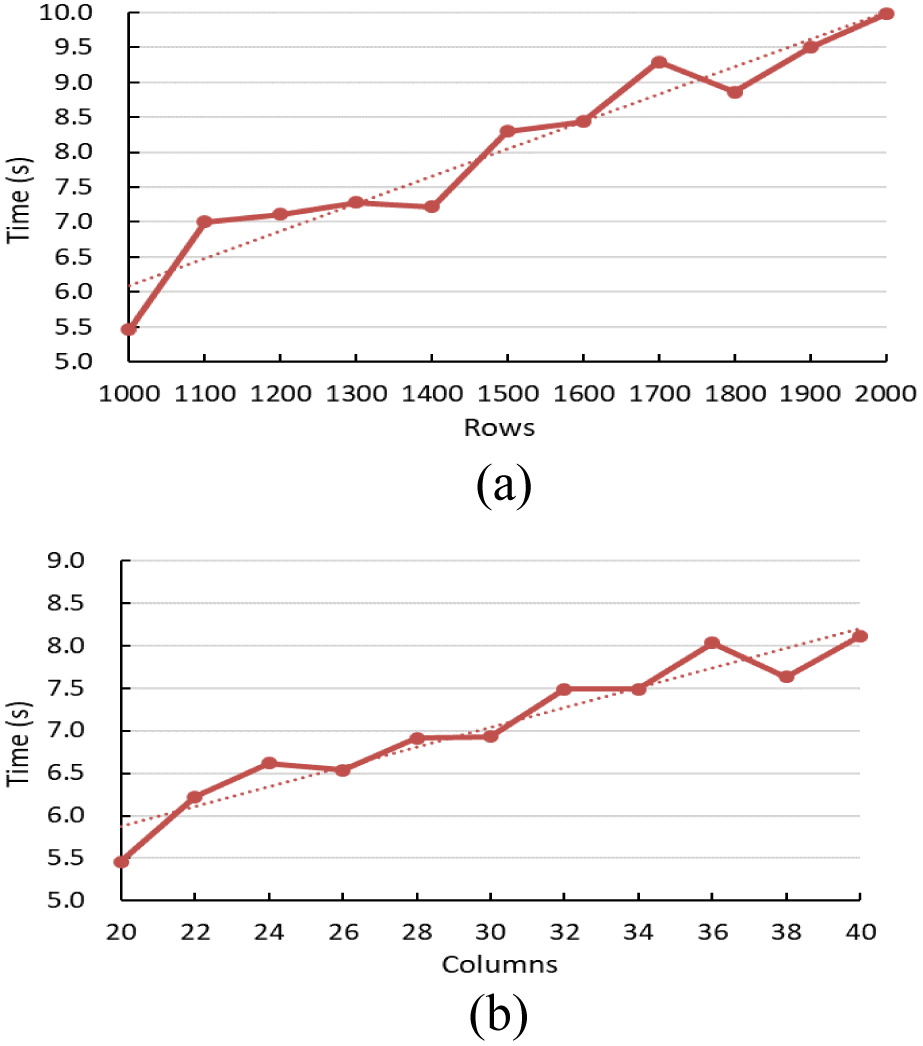Fig. 14. The relation between the run time and rows or columns.

It is also analysed the relationship between the running time of the algorithm and the number of rows of the data. A set of data sets are used whose number of columns are the same as 20. The number of rows of the data starts with 1000 and ends with 2000 with the increasing step 100. So there are 11 data matrices. The results are shown in Figure 15 (a). It can be seen from the graph that, on the whole, the run time of the algorithm increases linearly with the linear increase of the number of rows in the data, and the trend is shown by the dotted line in the Figure 15 (a).

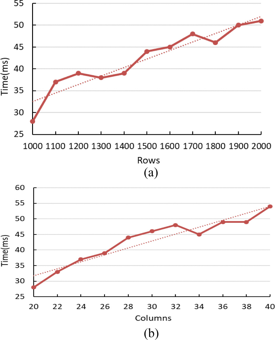Fig. 15. The relation between a single bicluster and rows or columns.

To analyze the relationship between the running time of the algorithm and the number of columns of the dataset, we use a set of data sets with the same number of rows (1000 rows). The number of columns of the data is set 20 as the starting point and 40 as the end point with the increasing step 2. Thus there are 11 data matrices. The results are shown in Figure 15 (b). As can be seen from the graph, in general, the execution time of the algorithm increases linearly with the linear rising of the number of columns in the dataset, as shown by the dotted line in the figure. Exceptionally, when the number of columns is 36, the running time is obviously longer than the number of columns 34 and 38 on both sides, because the number of double clusters generated is more. From the experimental results, we can see that BicACCC algorithm has good scalability in the case of increasing data volume.

2)Efficiency Analysis of the bicluster Mining

In order to achieve a more comprehensive performance of the algorithm, the relationship between the average time-consuming of mining each bicluster and the size of the data set is analyzed. The data used in the analysis is the same as the previous step’s. The experimental results are shown in Figure 16. The average time-consuming of each bicluster is linearly related to the number of rows or columns, as shown by dotted lines. In particular, when analyzing the relationship between the running time of the program and the number of columns, the running time is longer when the number of columns is 36, as shown in Figure 16(b), the time is not too long. That is to say, when the number of columns is 36, biclusters found are more. From the experimental results, it can be seen that BicACCC algorithm takes less time to mine each bicluster and has higher mining efficiency.

Fig. 16. Biclusters mined by BicACCC.

B.VISUALIZATION OF BICLUSTERS

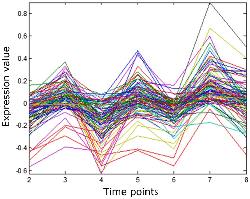
Firstly, the BicACCC algorithm proposed in this paper is used to mine biclusters. Based on the biclusters from the original sequential gene microarray data, the corresponding graph is drawn. From the graph, we can intuitively learn the common characteristic of the biclusters.

As shown in Figure 17, the abscissa in the graph refers to the label of columns of the biclusters, the different curves in the graph refer to different genes, and the ordinate in the graph refers to the expression values in the gene microarray data matrix. From the graph, we can see that the gene expression values in the bicluster showed the same trend of rise and decrease at the adjacent time points, that is, the change trend of gene expression values at the same group of adjacent time points is the same. From the graph, we can see that the bicluster obtained has obvious coherent properties.

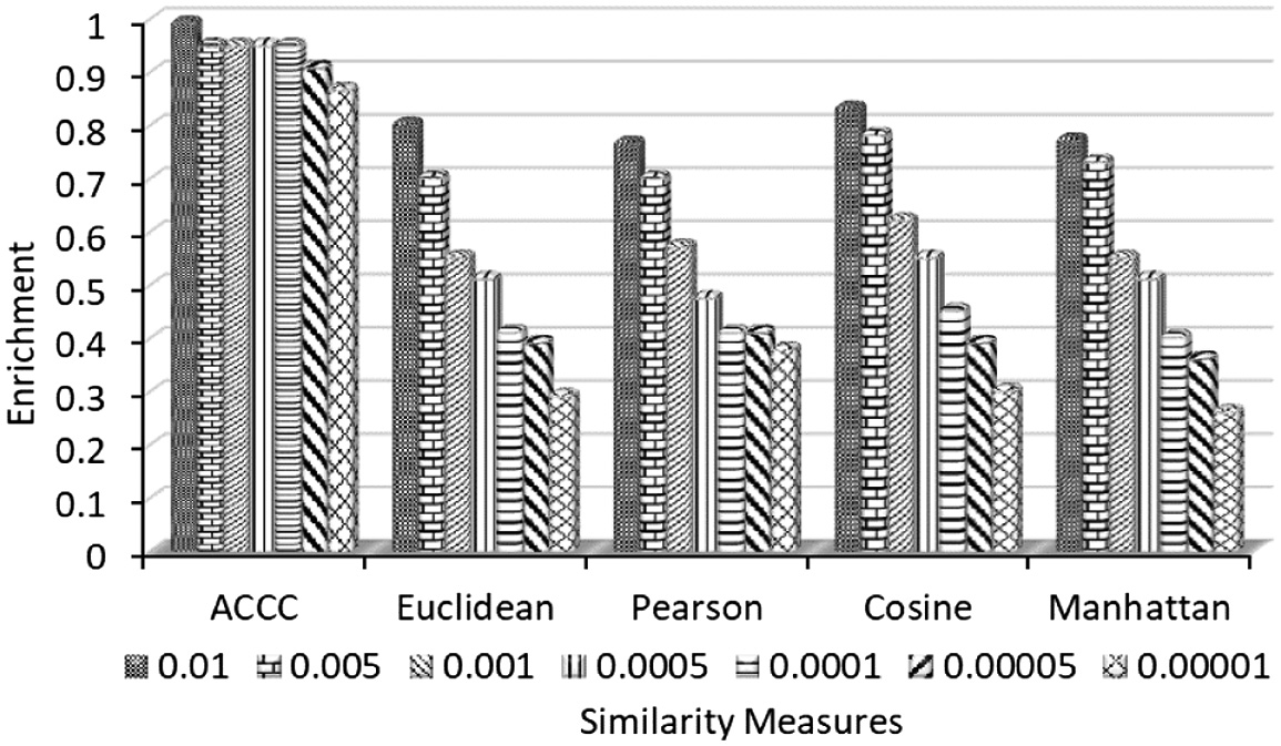Fig. 17. The comparison of enrichment on different similarity measures.

C.GENE ONTOLOGY ANALYSIS

Gene Ontology (GO) is a database created by the Gene Ontology Federation. It has the standard vocabulary of biological gene language. This standard aims to be used in various biological applications, to describe the functions of genes and proteins, and to be updated continuously. GO can be divided into three aspects: molecular function, biological process and cell composition. GO is often used to test the biological authenticity of clustering or biclustering results, that is, to reflect the biological significance of clustering or biclustering results.

In order to study the biological significance of the biclusters, the tool GOToolbox 0 is used to analyze. GOToolbox is a web application platform which can help researchers to query gene ontology data easily, and its annotated data can be visually displayed. So far, the GOToolbox project has covered a large database for genes such as animals and plants. We use GOToolbox tool platform to study the biclusters obtained in this paper. The analysis includes GO Term, GO Level analysis and so on.

In the experimental analysis of this paper, we use GOToolbox tool to get P-value of the biclusters. By studying GO annotations of genes belonging to the same category and calculating the biclusters found by the algorithm and the P-value of known gene types, we can understand the biological value of the biclusters.

Genes with same expression levels often belong to the same biological pathway, and their molecular functions and biological processes are somewhat similar. On the GOToolbox tool platform, the experiment of mining GO annotations with the biclusters is done to output the corresponding P-value. P-value is to find the possibility of a given gene annotation when the data distribution is known. The smaller the P-value is, the lower the possibility of finding a given gene annotation is. In fact, it can be found in the biclusters. Therefore, the biclusters have certain biological significance. The smaller the output P-value is, the closer the correlation between the bicluster’s patterns and the corresponding gene types.

P-value is calculated as the following:

P - v a l u e = \sum_{j = x}^{n} \frac{(\begin{matrix} M \\ j \end{matrix}) (\begin{matrix} N - M \\ n - j \end{matrix})}{(\begin{matrix} N \\ n \end{matrix})}

(8)

Where N refers to the total number of genes in the gene dataset; M refers to the number of annotations for N genes covered; n refers to the total number of genes in the bicluster; x refers to the number of annotations for x genes covered.

Take GO analysis of yeast microarray data as an example. The first line in Table 3 is GO:0002181. There are 7166 genes in the gene database, of which only 186 genes (2.6%) belong to GO in cytoplasmic translation. However, we find 754 genes in a bicluster found by BicACCC, 90 of which (11.9%) belonged to GO items of cytoplasmic translation. Calculated by the equation, the P-value is very small, which reflects the significance of the bicluster in biology.

Table III Go analysis of BicACCC biclusters in yeast microarray dataset

G0 ID	Gene Ontology term	Cluster frequency	Genome frequency	Corrected P-Value
G0:0002181	cytoplasmic translation	90 of 754 genes,11.9%	186 of 7166 genes,2.6%	4.62E–37
G0:0042254	ribosome biogenesis	124 of 754 genes,16.4%	470 of 7166 genes, 6.6%	7.05E–21
G0:0022613	Ribonucleoprotein complex biogenesis	138 of 754 genes, 18.3%	567 of 7166 genes, 7.9%	5. 93E–20
G0:0042274	ribosomal small subunit biogenesis	59 of 754 genes, 7.8%	145 of 7166 genes,2.0%	1.54E–18
G0:0042255	ribosome assembly	38 of 754 genes, 5.0%	73 of 7166 genes, 1.0%	1.06E–15
G0:0034460	ncRNA metabolic process	127 of 754 genes, 6.8%	570 of 7166 genes, 8.0%	1.41E–14
G0:0030490	maturation of SSU-rRNA	46 of 754 genes, 6.1%	117 of 7166 genes,1.6%	2.75E–13
G0:0000462	maturation of SSU-rRNA from tricistronic rRNA transcript (SSU-rRNA, 5.85 rRNA, LSU-rRNA)	42 of 7 54 genes, 5.6%	108 of 7166 genes, 1.5%	9.31E–22
G0:0034470	ncRNA processing	108 of 754 genes, 3.7%	460 of 7166 genes, 6.4%	2.07E–11
G0:0016072	rRNA metabolic process	87 of 754 genes, 1.5%	359 of 7166 genes, 5.0%	2.44E–11

The GO analysis results of yeast microarray data, mouse microarray data and human cell microarray data are shown in Table 3, Table 4 and Table 5. It can be seen from the table that the P-value obtained is generally very low. The results of tables reflect that the biclusters found have certain biological significance. Combining the GO analysis results of three gene microarray datasets, it proves that BicACCC algorithm can effectively mine the knowledge with remarkable biological significance.

Table IV Go analysis of BicACCC biclusters in mouse cell microarray dataset

G0 ID	Gene Ontology term	Cluster frequency	Genome frequency	Corrected P-Value
G0:0008152	metabolic process	627 of 1109 genes,56.5%	1023 of 24197 genes,42.2%	3.28E–19
60:0044237	cellular metabolic process	551 of 1109 genes,49.7%	8914 of 24197 genes,42.2%	1.08E–15
60:00099ft7	cellular process	820 of 1109 genes,49.7%	1023 of 24197 genes,42.2%	5. 93E–20
60:0044699	single-organism process	757 of 1109 genes,68.3%	13528 of 24197 genes, 55.9%	1.88E–14
60:0071704	organic substance metabolic process	567 of 1109 genes, 51.1%	9534 of 24197 genes, 39.4%	1.49E–12
60:004423ft	primary metabolic process	540 of 1109 genes,48.7%	9084 of 24197 genes, 37.5%	2.37E–11
60:0006ft07	nitrogen compound metabolic process	379 of 1109 genes,34.2%	5860 of 24197 genes, 24.2%	5.36E–11
60:0044710	single-organism metabolic process	304 of 1109 genes,27.4%	4437 of 24197 genes, 18.3%	7.12E–11
60:0034641	cellular nitrogen compound metabolic process	356 of 1109 genes, 32.1%	5595 of 24197 genes, 23.1%	6. 01E–09
60:0044763	single-organism cellular process	667 of 1109 genes, 60.1%	12149 of 24197 genes. 502%	2.50E–08

Table V Go analysis of human sell microarray dataset

G0 ID	Gene Ontology term	Cluster frequency	Genome frequency	Corrected P-Value
G0:0032501	multicelluar process	228 of 497 genes, 45.9%	7806 of 46271 genes,16.9%	3.39–48
G0:0044707	Single multicelluar organism process	221 of 497 genes, 44.5%	7527 of 46271 genes,16.3%	1.53E–46
G0:0044767	Single organism development process	186 of 497 genes, 37.4%	6428 of 46271 genes,13.9%	5.15E–36
G0:0032502	development process	187 of 497 genes, 37.6%	6523 of 46271 genes,14.1%	1.04E–35
G0:0007275	multicelluar organism process	168 of 497 genes, 33.8%	5394 of 46271 genes,11.7%	1.56E–35
G0:0050896	response to sti mulus	266 of 497 genes, 53.5%	12165 of 46271 genes,26.3%	7.84E–35
G0:0065007	biological regulation	329 of 497 genes, 66.2%	17941 of 46271 genes,38.8%	5.97E–32
G0:0048856	anatomic structural development	166 of 497 genes, 33.4%	5662 of 46271 genes,12.2%	9.86E–32
G0:0048513	organ development	122 of 497 genes, 24.5%	3223 of 46271 genes,7.0%	1.07E–31
G0:0048731	system development	149 of 497 genes,30.0%	4706 of 46271 genes,10.2%	2.54E–31

D.BIOLOGICAL ENRICHMENT ANALYSIS

In order to verify the biological significance of biclusters in the statistical sense, biological significance analysis can be carried out by analyzing the biological function enrichment of the biclusters [23]. By calculating the P-values of the biclusters and the known gene species, and counting the percentage of the biclusters, whose P-values are less than the preset P-value threshold, we can understand the enrichment of the biclusters in the biological process from the statistical point of view. The lower P-value settings and the larger the percentage is, the stronger the correlation between the biclusters and the known gene categories in general, which indicates that the biclusters are more significant in biology.

Firstly, in order to prove that the ACCC similarity measure proposed in this paper can measure the similarity of time series data very well, the enrichment analysis of the results is made. In this experiment, human cell microarray data were used. Using K-means algorithm in BicAT toolbox, we select the existing similarity measures such as Euclidean (Euclidean distance), Pearson (Pearson similarity coefficient), Cosine (cosine similarity), Manhatan (Manhattan distance) in the toolbox to calculate the corresponding enrichment ratio. Then, we run the K-means program using ACCC similarity measure, and we get the results for enrichment analysis as shown in Figure 18.

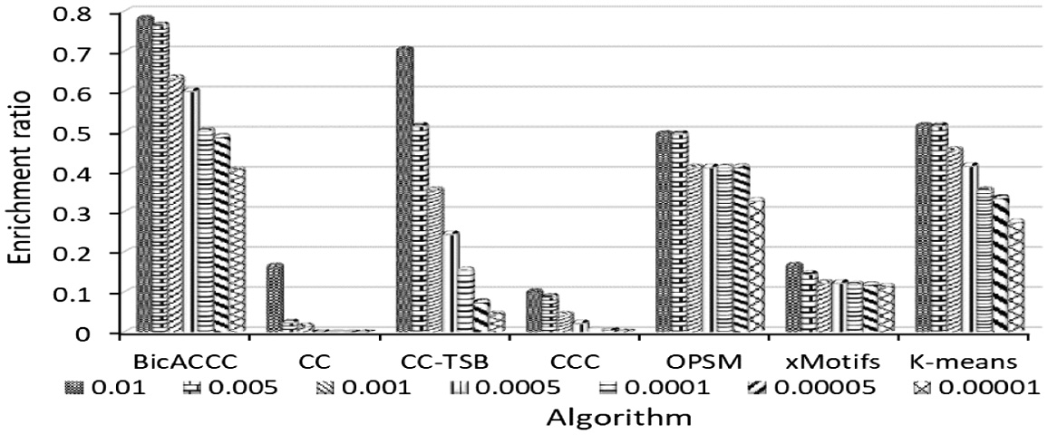Fig. 18. The enrichment ratio of different algorithm in yeast microarray data.

From the graph, it can be seen that the results of similarity measure ACCC are better than those of Euclidean, Pearson, Cosine and Manhatan. For example, when the P-value threshold is 0.01, the enrichment ratio of ACCC results is 1, while the highest results of other similarity measures are Cosine 0.84, which is less than 1. When P-value is small, the advantage of ACCC is more obvious. For example, when P-value threshold is 0.00001, the enrichment ratio of ACCC results is 0.88, while Pearson is 0.39, which is significantly less than 0.88. The experimental results show that the similarity measures of ACCC are better than those of Euclidean, Pearson, Cosine and Manhatan in the sequential gene microarray data.

In order to compare and evaluate the results of BicACCC algorithm on biological enrichment, we select CC, CC-TSB, CCC, OPSM, xMotifs, K-means algorithms in BicAT toolbox. Then, the results of CC, CC-TSB, CCC, OPSM, xMotifs and K-means are obtained. The enrichment results of statistics are drawn on the figures.

The results of yeast microarray data are shown in Figure 19. It can be seen from the graph that the enrichment ratios of BicACCC algorithm under different P-value thresholds are higher than that of other algorithms under the same corresponding threshold. For example, when the P-value threshold is 0.01, the enrichment ratio of BicACCC algorithm is 0.78. The results of CC, CC-TSB, CCC, OPSM, xMotifs and K-means are 0.17,0.71,0.11,0.5,0.17,0.52 respectively, which are less than 0.78. When P-value is small, the advantage of BicACCC algorithm is more obvious. For example, when P-value threshold is 0.00001, the enrichment ratio of BicACCC algorithm is 0.41. The results of CC, CC-TSB, CCC, OPSM, xMotifs and K-means are 0, 0.05, 0.01, 0.33, 0.12, 0.28 respectively, which are smaller than 0.41. In the dataset, the biological enrichment of the biclusters mined by BicACCC algorithm is better than other algorithms’ on the whole.

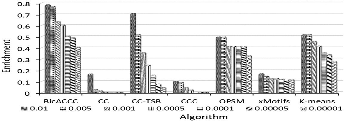Fig. 19. The comparison of enrichment in mouse cell microarray data.

As for mouse cell microarray data, we can see from Figure 20 that the biclustering enrichment of BicACCC algorithm is significantly higher than that of CCC, CC-TSB, CCC, OPSM, xMotifs and K-means. In particular, both CC and CCC algorithms perform poorly and are not suitable for this data set.

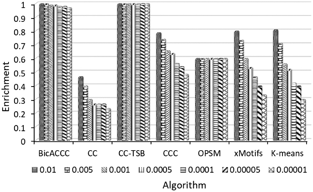Fig. 20. Comparison of enrichment in mouse cell microarray data.

For human cell microarray data, as shown in Figure 21, all of these algorithms perform well. BicACCC algorithm’s results are slightly inferior to CC-TSB algorithm’s results, but the results of BicACCC algorithm are obviously better than the other five algorithms.

The enrichment analysis of real gene microarray data sets shows that BicACCC algorithm can obtain more valuable and biologically meaningful biclusters from gene microarray data.

VI.CONCLUSIONS

In the analysis of gene microarray datasets, a large number of biclustering algorithms did not account the temporal correlation of sequential gene microarray data. Considering the continuous time variation, the consistent evolution pattern in continuous columns could be mined. However, there was not a suitable similarity measure proposed for the consistent evolution in continuous columns, nor was the consistent evolution pattern in all continuous columns taken into account. In this paper, we first proposed a uniformly similarity measure, which measures the consistent evolution pattern in all continuous columns. According to the similarity measure, a biclustering model was proposed to mine all continuous columns coherent patterns. Firstly, the original data was transformed into the differential data, and then the initial core of the bicluster was defined. By using the measure function of biclusters, the high quality biclusters were found by iteration. In the experiments, the synthetic data sets were applied in simulation to analyze the performance of the algorithm, which shows that the proposed algorithm was efficient. Real gene microarray data sets were used to analyze the experimental results and verify the biological significance of the biclusters.

A Coherent Pattern Mining Algorithm Based on All Contiguous Column Bicluster