I.INTRODUCTION
The purpose of the overall project is to create a simulated environment similar to Google Maps, where live traffic data are fed into the map system that can be dynamically updated to display the quickest path to a particular destination. Google’s system is one of the best navigation solutions, but it is also too complex for introductory computer science students to create similar systems for learning purposes. A simplified traffic simulator environment was implemented, so that students could learn to program a virtual car with dynamically changing traffic. The main motivations of this paper are the presentation of a dataset creation process based on real traffic data and a corresponding dynamic routing algorithm for educational purposes.
The environment used in the project is ASU Visual IoT/Robotics Programming Language Environment (VIPLE) [1]. VIPLE offers all the functions necessary for novice programmers to learn programming concepts while experienced computer science students are able to program complex IoT devices, robots, and machine learning (ML) [1–3]. Various simulators have been implemented in VIPLE, including both desktop simulators and web simulators [2]. Traffic simulation is one of the functions that has recently been added into the VIPLE environment. VIPLE is particularly suited to this project as it provides strong support for orchestration and workflow in robotic applications [1,4].
This paper focuses on the traffic simulator, which is a desktop simulator, developed using the Unity game engine. The simulator provides an aerial view layout of a city grid and contains several different subareas of the city. Noncontrollable cars are colored yellow and are spawned by the simulator at any position on the road with randomized driving directions. These cars are used to represent traffic and can be given specific driving patterns according to supplied data. The red car can be programmed, for example, using VIPLE, and allows users to develop both manual and autonomous driving applications.
To provide a strong educational experience for computer science students, a number of student teams have engaged in developing the Unity traffic simulator. This project focuses on dynamic traffic routing on the traffic simulator using traffic data generated from real Maricopa County traffic data from 2020. This work aims to help students visualize their pathfinding algorithm using VIPLE and the traffic simulator. The data employed in this project are generated according to manually specified patterns from the original Maricopa County data. A self-sufficient approach can be implemented using an online ML application. Section VI provides more information on this topic.
Section II provides a review of the previous work that provides the foundation for this project. Section III details the outline of this project. Section IV outlines the method and implementation including a description of the generation of traffic data, operation of the traffic simulator, and a dynamic routing algorithm. Section V discusses and presents the results followed by a discussion of the contribution. Section VI concludes the paper with a discussion on potential future work.
II.RELATED WORK
This section presents related studies that have been done by Arizona State University faculty and students within the same overall project, as well as work done by researchers and practitioners from other organizations.
A.TRAFFIC SIMULATION
According to the definition from Wikipedia, “traffic simulation is the mathematical modeling of transportation systems through the application of computer software and graphic presentation to better help understand, plan, design, and operate transportation systems” [5]. Today, many traffic simulators exist, some of them are proprietary systems and others are open-source systems. For example, Anylogic [6] and TransModeler [7] are commercial software. Simulation of Urban Mobility (SUMO) [8], CityFlow [9], and OpenTrafficSim [10] are open-source simulators.
The software used as the main reference is SUMO, which has been developed by the Institute of Transportation Research at German Aerospace Center since the year 2000 [11]. The goal of SUMO is for traffic management and traffic forecasting [12], whereas the VIPLE simulator is intended for educational purposes focusing on programming logic and visualizing graphic algorithms. SUMO’s road network is similar to the VIPLE traffic simulator in that both use a graph data structure for the map. The roads are represented as edges and intersections are represented as vertices (nodes) [13]. SUMO uses a microscopic traffic simulation model which means that each vehicle on the street is simulated individually [14,15]. ASU VIPLE can be considered as using a macroscopic model, since it simulates the overall traffic situation, including traffic density and spawning rate, rather than the specific details of each car. Krauß discussed the traffic flow of SUMO in [16]. SUMO uses a microscopic traffic model in which traffic flow is also at the microscopic scale. The maximum safe velocity and acceleration for each car are important factors to be considered in traffic flow [16–18]. VIPLE’s traffic simulator does not consider these factors from the microscopic scale, focusing instead solely on the macroscopic scale. As a result, simulation and analysis become simpler at the cost of lower realism. Behrisch et al. introduce research topics related to SUMO vehicle-to-infrastructure communication, route choice, and traffic light algorithms in [11]. These elements have a certain similarity with VIPLE’s traffic simulator but with different approaches and goals.
B.TRAFFIC DATA GENERATION
Traffic data generation plays an essential role in this project and other research and applications. However, missing data is commonly encountered and typically causes problems in traffic data generation. Much research has been dedicated to solving data imputation problems. For example, bidirectional recurrent neural networks can be used to generate missing data in consecutive time periods [19]. Convolutional neural networks are models to compute the spatiotemporal missing traffic data [20,21]. Graph neural networks also can be used in spatiotemporal missing data. Zheng et al. proposed a graph multi-attention network to predict future traffic conditions [22]. In addition, a graph attention convolutional network was proposed by Ye et al. whose study suggested to “incorporate graph attention mechanism to learn spatial correlation of the traffic data,” then “temporal convolutional layers are stacked to extract relations in time-series after graph attention layers” [23]. A recent study summarized the previous works on missing patterns and missing traffic data imputation and addresses two limitations on the traffic data imputation in the previous works. The solution from that research is to combine the bidirectional recurrent layer with a graph-based convolution layer to model the spatiotemporal dependencies [24]. To facilitate visualization and presentation of the techniques and data, we employed a different approach as discussed below. However, these techniques can be used to enhance our approach in managing incomplete data.
C.VIPLE
VIPLE is a graphical programming language environment developed in our previous work. A VIPLE program “is represented as a workflow diagram, and the components are defined as activities or Web services in the diagram” [25]. These programs can be mathematically modeled using the Pi-Calculus, enabling automated semantic verification of decentralized IoT and robotics applications written using VIPLE [3,25]. The ability to perform such verification on student programs provides additional benefit to this system as an educational platform. Figure 1 shows the basic activities in VIPLE.
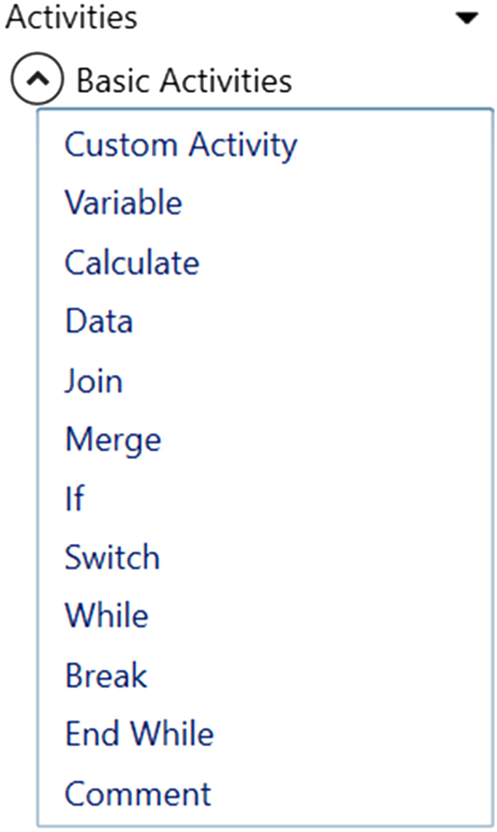 Fig. 1. VIPLE Basic Activities [25].
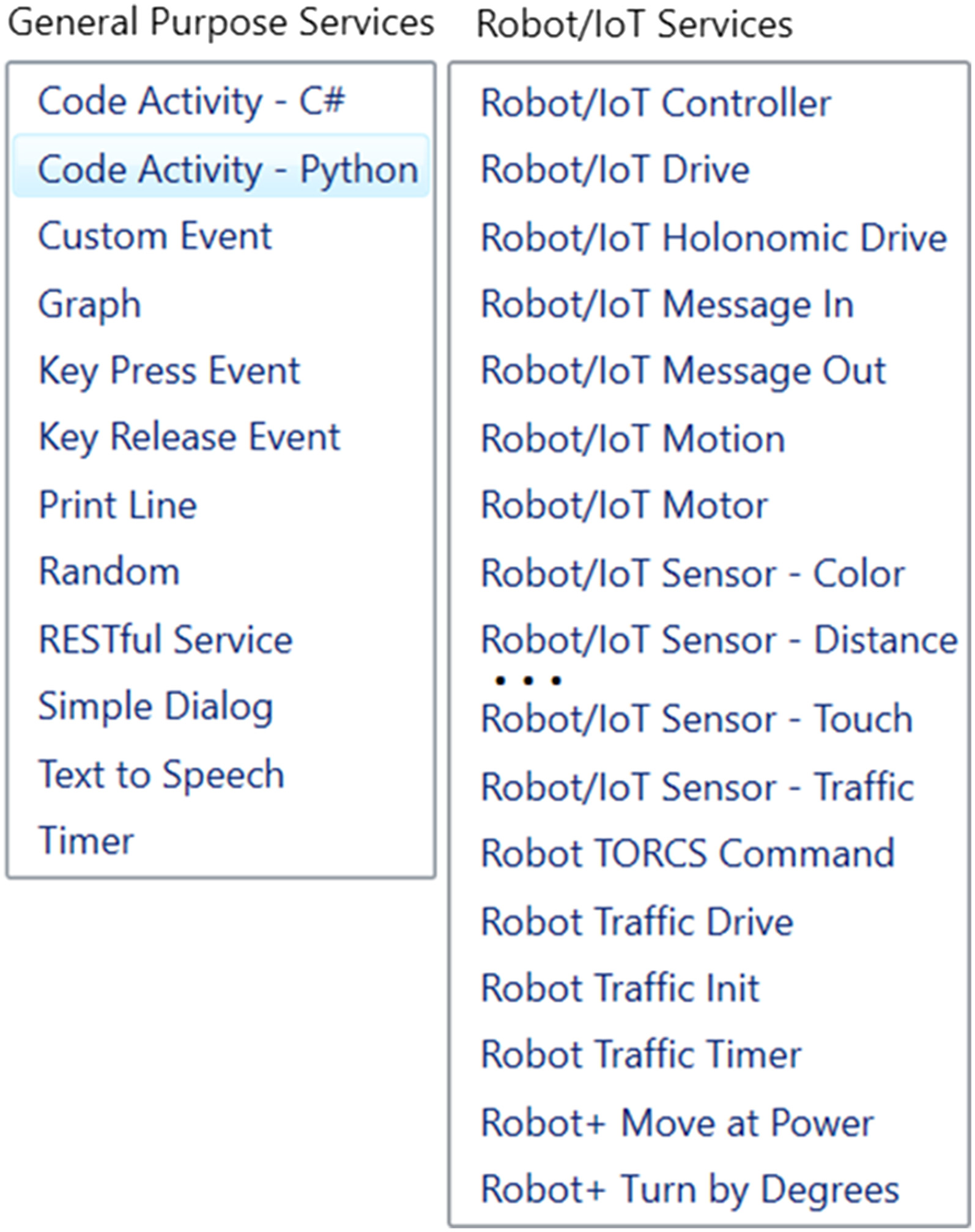
In addition to the basic activities, VIPLE provides various services to facilitate different types of teaching and research projects. Figure 2 presents two more sets of services that are used in this paper. The first set of services includes general services, including input/output services (Simple Dialog, Print Line, Text to Speech, and Random), event services (Key Press Event, Key Release Event, Custom Event, and Timer), and RESTful services. The second set includes Robot/IoT services. Communication types between VIPLE and Robot/IoT devices include Wi-Fi (TCP or WebSockets), Bluetooth, and USB interfaces. JavaScript Object Notation (JSON) is the data format VIPLE and Robot/IoT devices use to send or receive messages, though custom interfaces can be defined. These features provide the foundation for the current paper to develop a dynamic path planning algorithm in the VIPLE environment. ASU VIPLE can be downloaded from this site: http://venus.sod.asu.edu/VIPLE.
III.DESIGN
This section presents the overall design of the project, which includes the ideas and methods used.
For this project, real traffic data were employed in VIPLE’s traffic simulator from the local area, Tempe, Arizona, located in Maricopa County [26]. Although this traffic dataset is incomplete, it provides records of partially complete hourly traffic data for individual intersections. These data records facilitate the application of the data to the VIPLE traffic simulator.
With the dataset selected, the next step is to generate traffic data. Because of the incompleteness of the traffic dataset from the Maricopa government website, the data generation was based on partially complete data, according to the hourly traffic trend in previous research. Specifics of this data generation are presented in Section IV.B. This data generation step was completed manually for each road and each time interval. Due to the large values of the generated traffic data, the dataset could not fit into the traffic simulator at the original scale. It was therefore scaled down before integration. Subsequently, the roads were mapped to the traffic simulator according to the appropriate geographical position in Maricopa County. This generated traffic data, a complete and scaled dataset using the values from real traffic data, was incorporated into the traffic simulator through the JSON data format and the Unity platform where the traffic simulator was developed. Lastly, the path planning algorithm, Dijkstra’s algorithm, was implemented in the VIPLE environment using a min-heap data structure. In a classroom environment, various shortest path algorithms may be substituted. Dijkstra’s algorithm was arbitrarily chosen for this work to provide a baseline demonstration of the work.
The experiment for this project is to run Dijkstra’s algorithm with the city’s simulated dynamically changing traffic patterns. The global path for the VIPLE programmable red car that defines the navigation path to the destination continually updates at each new intersection, demonstrating the quickest route according to the distance and traffic congestion on the roads at the given time.
IV.IMPLEMENTATION
This section illustrates the implementation process in detail, including generating traffic data, incorporating traffic data into the simulator, and implementing a dynamic version of Dijkstra’s path planning algorithm in VIPLE.
A.TRAFFIC SIMULATOR OPERATION
This section introduces some functionalities and features of the traffic simulator that were used in this project.
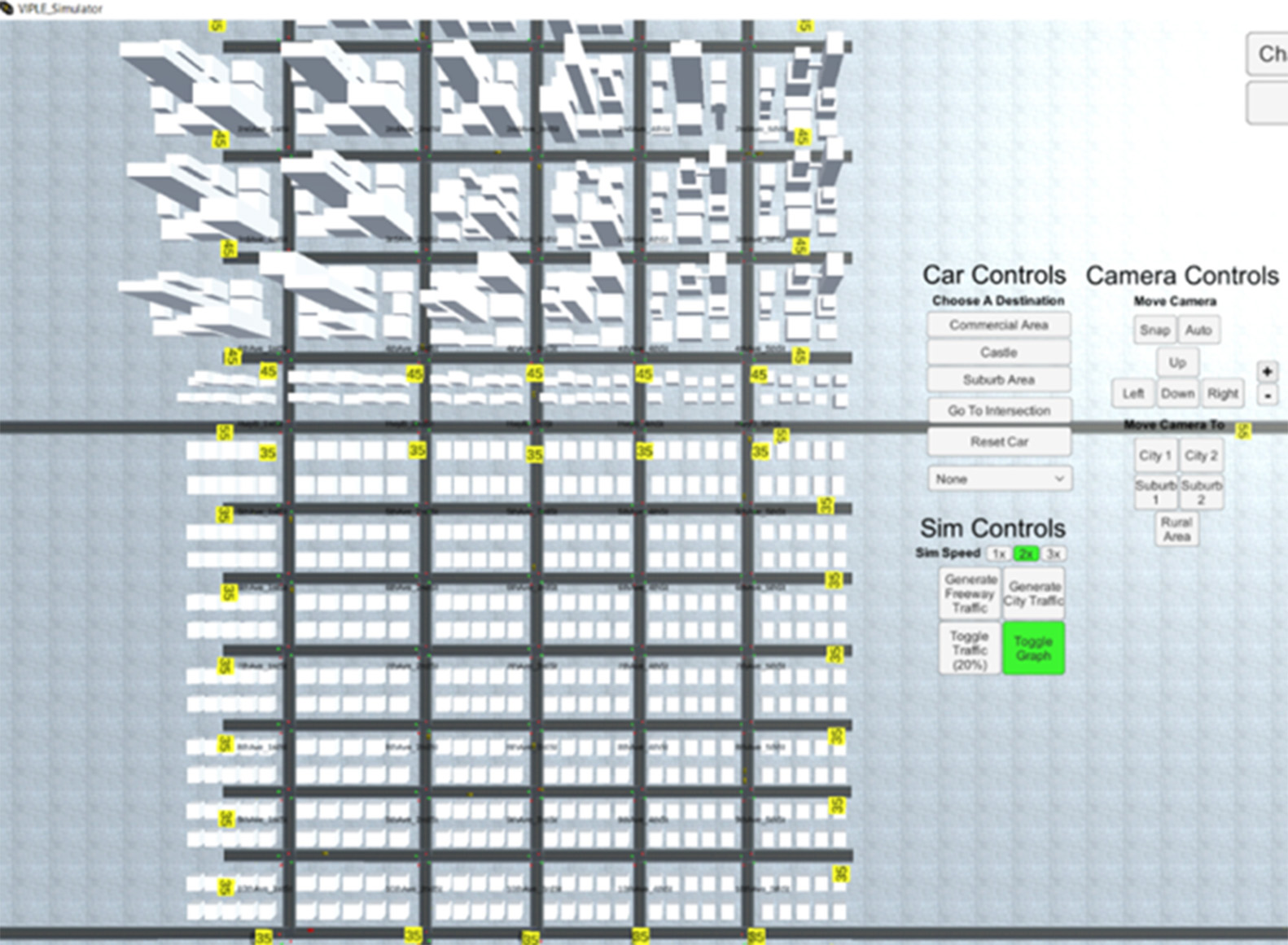
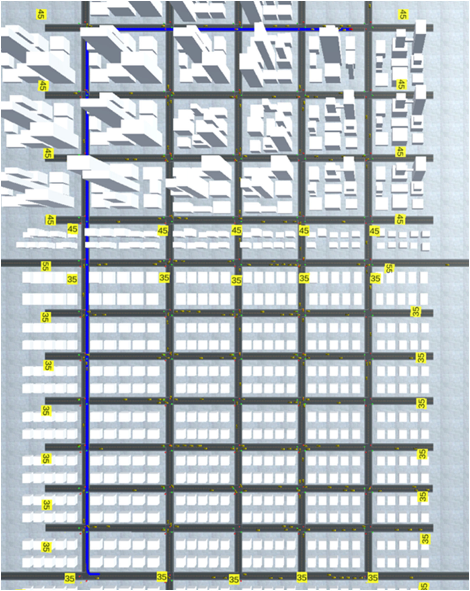
1)DATA STRUCTURE OF THE TRAFFIC SIMULATOR MAP
As shown in Fig. 3, the traffic simulator is arranged in a grid. As a result, the current simulator only supports streets that match this layout, though further work could support more types of roads. The entire traffic simulator map is stored as a graph data structure. Each road is stored as an edge, and intersections are represented as vertices. The adjacency list is formed by the neighboring intersections of each intersection. The weight of each segment of road is represented as a combination of the Manhattan distance and number of cars on the road. The integration of this information into the simulator is detailed in Section IV.D.
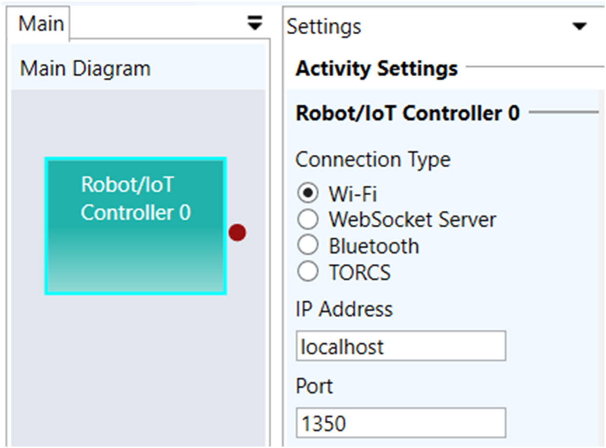
2)COMMUNICATION WITH A VIPLE PROGRAM
To enable communication between VIPLE and the traffic simulator, the Robot/IoT Controller service needed to be configured properly. Figure 4 presents the configuration applied for this project. Robot/IoT Message In is a service that can receive custom JSON messages from the traffic simulator by listening on the socket defined in the Robot/IoT Controller configured earlier. Robot/IoT Message Out is used to transmit JSON messages through the socket to the traffic simulator. The traffic simulator receives the JSON messages and responds accordingly.
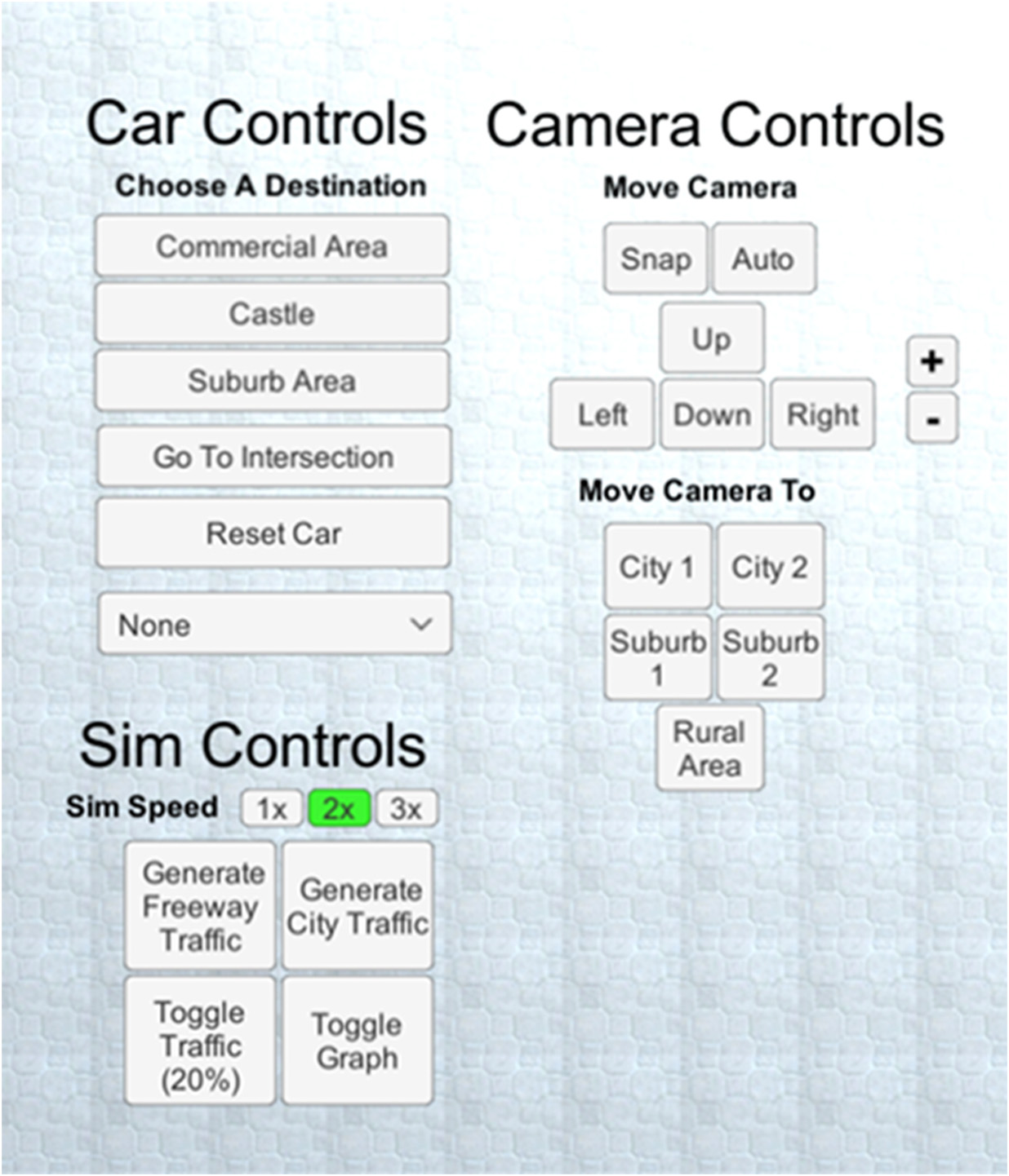
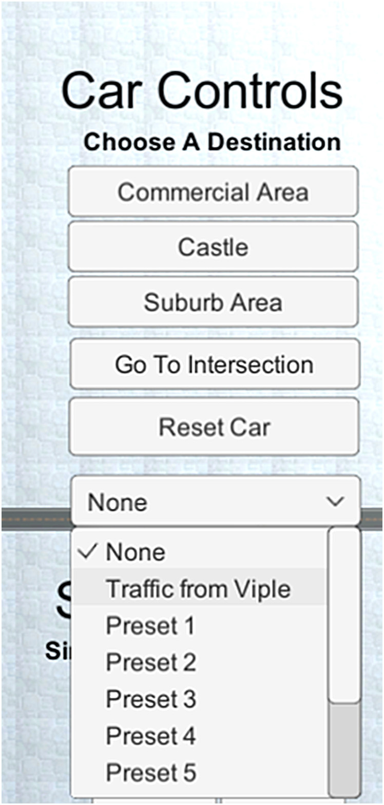
3)THE TRAFFIC SIMULATOR’S CONTROL INTERFACE
The main control buttons are shown in Fig. 5. The Car Controls section’s buttons take the red car to the designated area of the map. The dropdown list includes different traffic patterns that control the number of yellow cars on the map, corresponding to the traffic density set for the simulator. Camera Controls help to navigate the traffic simulator to different areas. The WASD keys may also be used to pan the map north, west, south, and east, respectively, Z can be used to zoom in, and X can be used to zoom out. Toggle Traffic from the Sim Controls section toggles the yellow cars to spawn at 0%, 20%, or 50% spawn rates. Toggle Graph shows each intersection’s name on the graph.
B.MARICOPA COUNTY TRAFFIC DATA GENERATION
The purpose of this section is to present the Maricopa County traffic data, describe how to overcome the incomplete data problem to generate traffic data, and the approach used to match the real traffic data to the VIPLE traffic simulator.
The data used in this project are from the Maricopa County government website. Fig. 6 shows a small sample of the data. This dataset contains 1378 records of various intersections’ traffic information at different times of day. For example, the record in the 3rd row of the table shows that on August 26, 2020, at the intersection of Carefree Hwy and 7th Ave, 5893 cars drove north on 7th Ave through the intersection. At 8:15, 427 cars passed through this intersection heading north, while 533 cars did the same at 15:45.
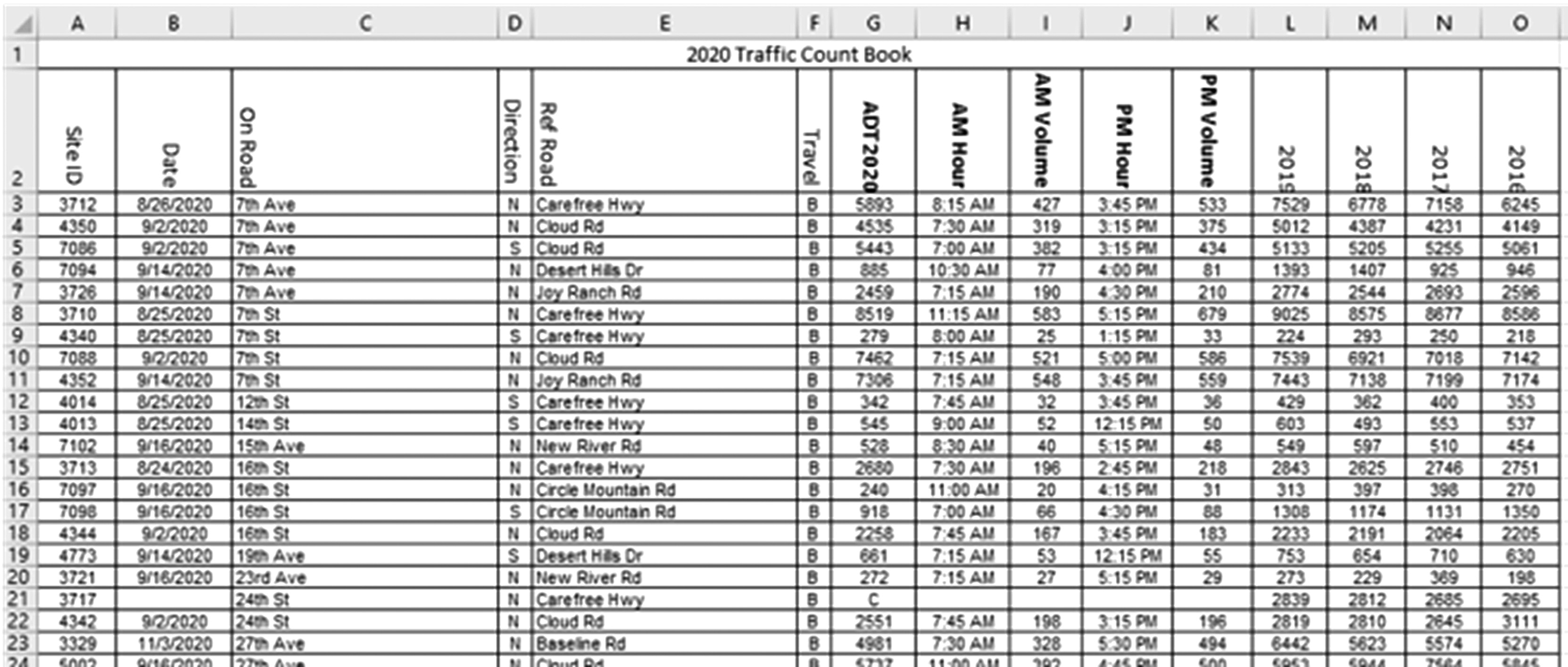 Fig. 6. Maricopa County Traffic Data.
Considering many major roads in Maricopa County follow a grid layout, the traffic simulator was created using an 11 × 5 grid as shown in Fig. 3. This structure was chosen to enable the application of local traffic patterns. According to this 11 × 5 grid in the simulator, eleven roads run in the east and west (E/W) direction, and five roads run in the north and south (N/S) direction. Maricopa County traffic data needed to be chosen and matched to the 11 × 5 simulator grid. However, a direct translation was impossible as the Maricopa County government website is not complete in the following ways. First, the dates to record Maricopa County traffic were not complete. For this traffic dataset, most of the records were for weekdays. Second, hourly traffic in a day was incomplete. For example, one intersection may only have contained traffic records at 8am and 4pm for that day. Third, one intersection may only have had traffic records for one direction. For example, the dataset only recorded the number of cars going north at the 7thAve and Carefree Hwy intersection but omitted traffic records for the south, east, and west directions.
With acknowledgement of the incompleteness of the dataset, the next step was to clean and process the traffic dataset from the Maricopa County website, mainly using the pandas Python library. First, rows containing empty cells were removed. By removing these rows, the traffic records were reduced from 1378 rows to 1278 rows. The data in the columns of Date, AM Hour, and PM Hour were originally represented as strings. In order to do computation on time in the future, the to_datetime function from pandas was used to convert the Date, AM Hour, and PM Hour into a date and time format recognized in Python.
Once the traffic data were cleaned, selecting proper traffic data records became an essential task. Eleven roads running east and west and five roads running north and south were chosen from Maricopa County traffic data to match to the traffic simulator. The first attempt included selecting major streets from the local area. However, this approach was not successful due to the incompleteness of the data because one intersection only had traffic records for one direction.
To resolve this issue, we selected roads and intersections from the dataset which had as much complete information as possible. Then, based on the records from the dataset, we generated traffic data according to hourly traffic trends in a given day [27]. According to the dataset, the west area of Maricopa County included more complete data records. Thus, roads were chosen mainly from the west area of Maricopa County. N/S roads included 355th Ave, Jackrabbit Tr, El Mirage, 107th Ave, 99th Ave and E/W roads included Thunderbird Blvd, Peoria Ave, Camelback Rd, Indian School Rd, Van Buren St, Buckeye Rd, Lower Buckeye Rd, MC 85, Broadway Rd, Southern Ave, Baseline Rd, Dobbins Rd, Elliot Rd. The isin function was used from pandas to select the records that have roads running in the N/S direction. These were designated as On Road. E/W roads were set as Ref Road. Other records had roads running in the E/W direction delineated as On Road and roads running in the N/S direction that were Ref Road. The records after processing are shown in Fig. 7.
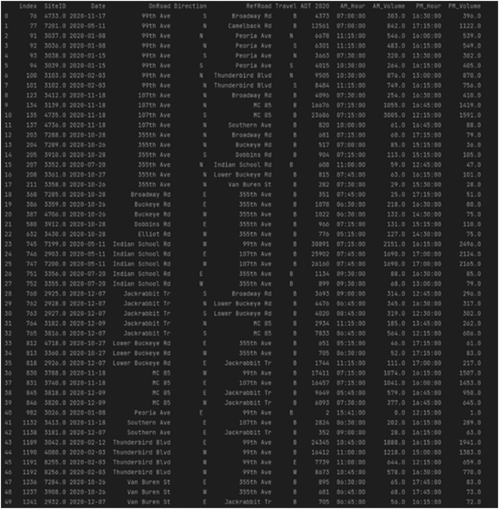 Fig. 7. Selected Traffic Data from Arizona Maricopa County.
With the selected records from the dataset and hourly traffic graphs obtained using the same method as described by [27], traffic data generation proceeded. The next step of data generation was completed manually for each road for different time durations. The daily traffic trends were split into eight distinct time groups. The eight different groups are: 0:00–5:00, 5:00–8:00, 8:00–12:00, 12:00–14:00, 14:00–17:00, 17:00–19:00, 19:00–21:00, and 21:00–23:59. To manually generate a complete traffic dataset, we analyzed the existing Maricopa County traffic data for each road. Then, based on the existing traffic data, we applied traffic patterns as linear functions with a random component to obtain the whole day traffic data for a specific road. Figure 8 presents sample code illustrating how traffic data were generated for Thunderbird Blvd for eight different time periods in a day. First, as shown in Fig. 7, #43 to #47 are the records that have Thunderbird as On Road. Available times in records for Thunderbird are 10:45, 11:00, 12:15, 15:00, 16:15, and 16:30, which fall in the 8:00–12:00, 12:00–14:00, and 14:00–17:00 durations. It should be noted that for manual traffic generation, the dates do not play an important role in this process because most of the dates are on weekdays and the goal for the traffic data generation is to generate hourly traffic for any of the weekdays. The highest number for 10:45, during the 8:00–12:00 duration, is 1888, and the lowest number is 578. The highest number for 11:00 is 1218, and the lowest number for 11:00 is 644. According to the traffic trend from Fig. 8, the traffic slightly decreased from 8:00 to 12:00 during the weekday. Thus, the linear function for 8:00–12:00 is shown in Equation 1 below, where rand_time is the time randomly generated between 8:00 and 12:00. Though this formula does not perfectly model the values in the real data, it provides similar ranges based on the ranges from the real dataset in each time range.
Then, we added randint (0, 1400) to the linear function because for the time duration between 8:00 and 12:00, the maximum difference for the same hour at 10:45 was 1888–578, which is 1310. A random number is used in the total traffic to take different traffic situations for different days into consideration. For the time duration omitted in the Maricopa County traffic data, the hourly traffic trend graph from Fig. 8 is applied to the linear function. For instance, the traffic for Thunderbird Blvd between 5:00 and 8:00 is missing. According to the existing traffic data from 8:00 to 12:00, the traffic at 8:00 is between 1000 and 2400. Also, the increase rate for 5:00–8:00 is faster. Thus, the linear function used is shown in Equation 2, with a random integer between (0, 1400). This formula demonstrates the same ideology as Equation 1 for a different time range.At 8:00, the traffic increased between 1000 and 2400 with 250 cars per hour. This process is repeated for other time durations in a day for Thunderbird Blvd. Then, other roads used the same idea to generate traffic data at different hours.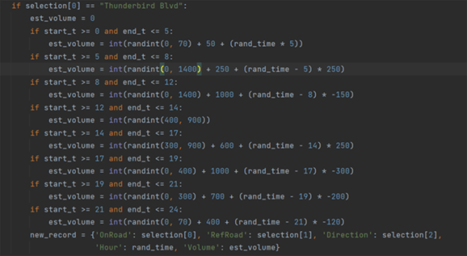
C.MAP MARICOPA COUNTY TRAFFIC DATA TO TRAFFIC SIMULATOR
Determining how the Maricopa County traffic data map to the traffic simulator was the next task. The mapping process was performed in two major steps. The first step was to map the roads from Maricopa County to the simulator geographically. The second step was to correspond the hourly traffic data for each road in the simulator.
The first step of the mapping process was straightforward because the chosen roads in Maricopa County were mapped to the same geographical position in the traffic simulator as much as possible. Figure 9 shows the mapping from the Maricopa County roads to the simulator roads. The yellow columns show the roads that run in the N/S direction, and the green rows show the roads that run in the E/W direction.
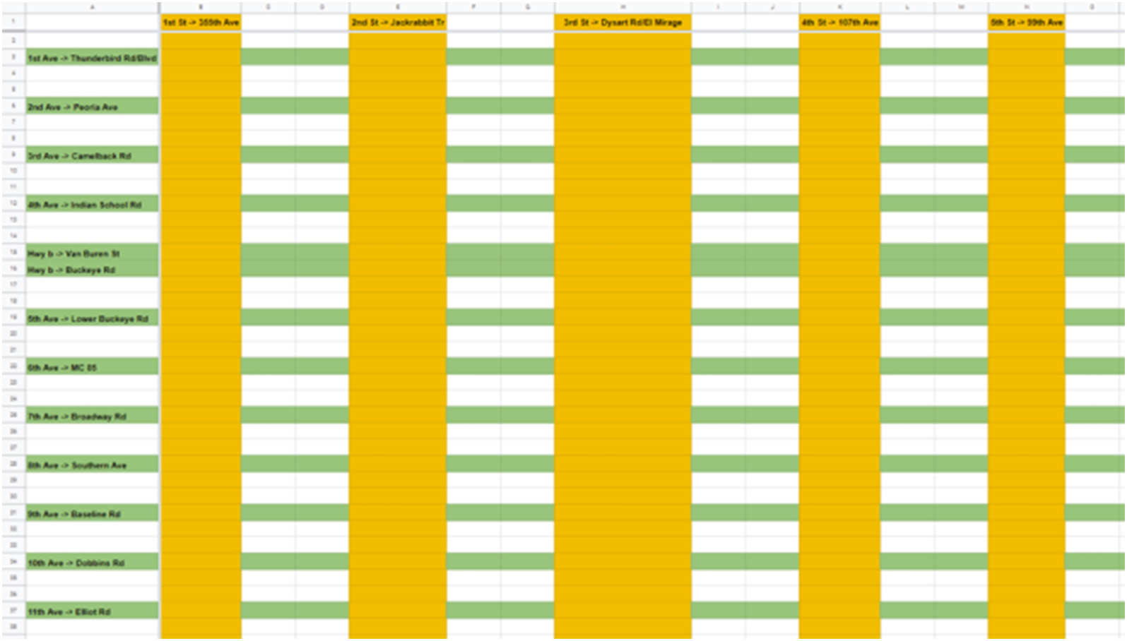 Fig. 9. Mapping between Maricopa Roads and Simulator Roads.
The second step of mapping was necessary because the real traffic data from Maricopa County were too large for the traffic simulator. To have traffic data that the simulator could process, we had to scale down the Maricopa County traffic volume. The traffic volume for each road in Maricopa County varies from 20 to 3000. To scale down, we divided all the original traffic data by 100. Then, we grouped the resulting values from 0 to 30 into ten intervals and assigned the appropriate volume value of each interval to each traffic simulator road as presented in Fig. 10.
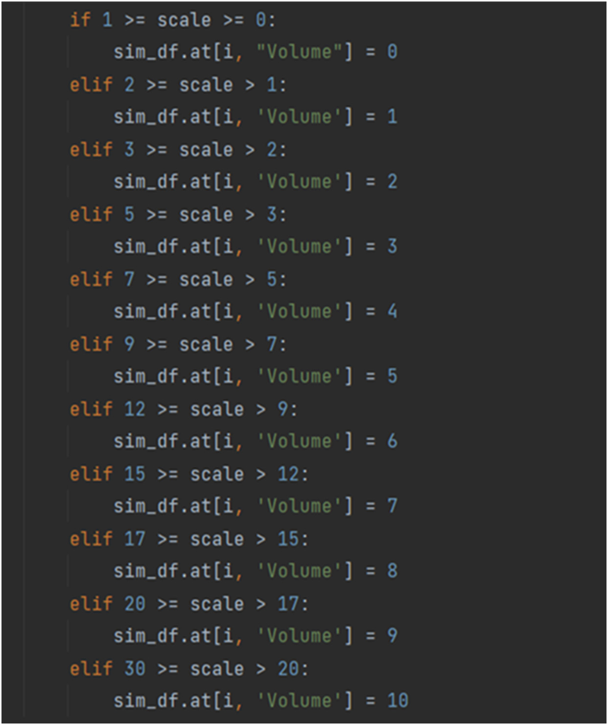 Fig. 10. Scale Down Traffic Data in Ten Intervals.
Figure 11 presents how the traffic data changes hourly as a whole for the scaled-down data.
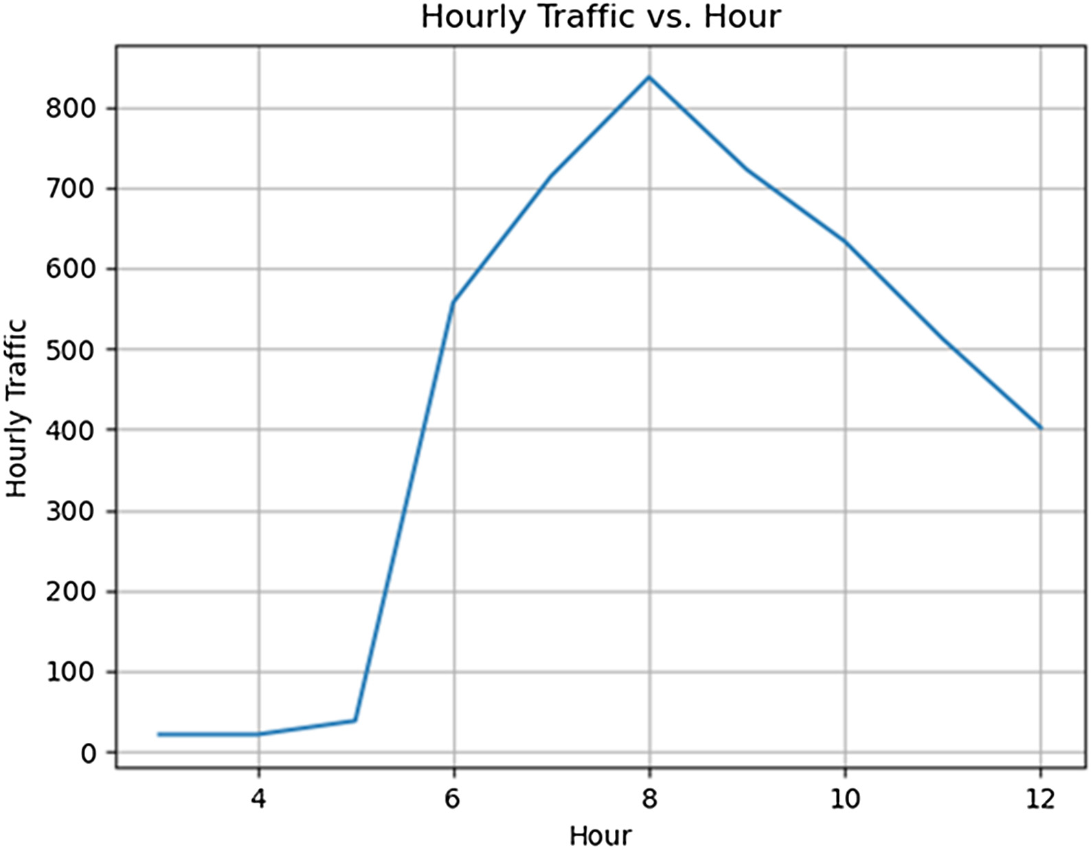 Fig. 11. Hourly Traffic for Simulator vs. Hour.
Finally, since the traffic data generated in Python were in a pandas DataFrame object, which cannot be directly sent to the simulator, the traffic data needed to be changed to JSON format. A sample JSON file that includes 7:00–8:00 traffic data is shown in Fig. 12.
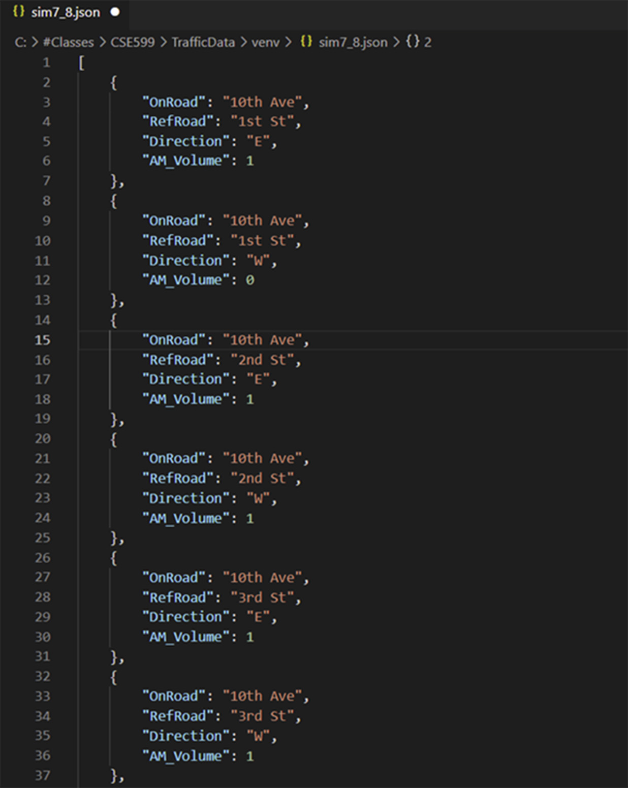 Fig. 12. Sample JSON File Showing Traffic Data Between 7:00 and 8:00.
D.INCORPORATE GENERATED TRAFFIC DATA INTO TRAFFIC SIMULATOR
The traffic simulator map was stored as a graph data structure. Roads were represented as edges and intersections were represented as vertices of the graph. Neighboring intersections for each vertex were included in the adjacency list. Code in Fig. 13 demonstrates the JSON structure sent from the simulator.
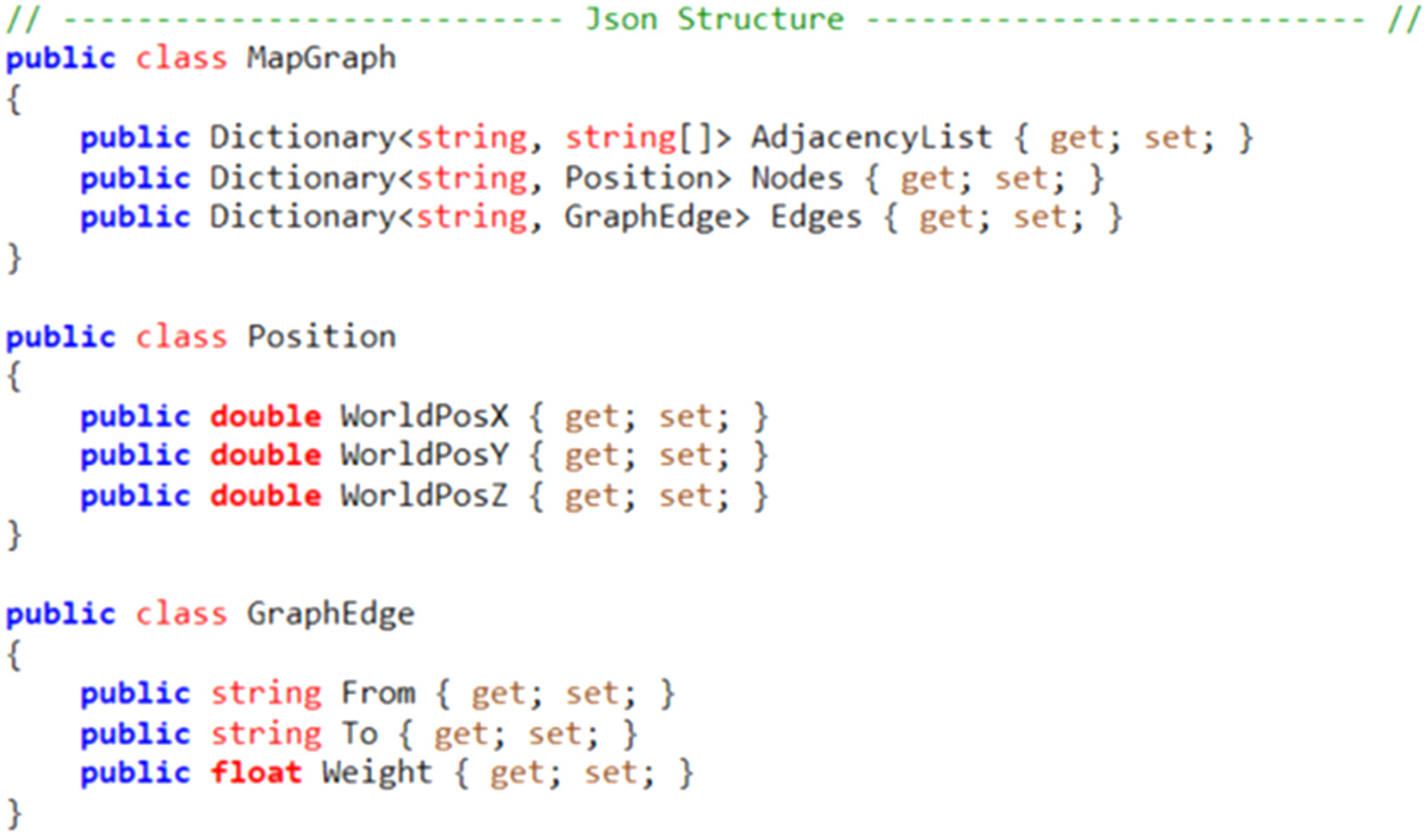 Fig. 13. JSON Structure of Traffic Simulator.
The senior capstone team at Arizona State University in charge of developing the traffic simulator helped create a preset dropdown list to select hourly traffic patterns in the simulator, as shown in Fig. 14. “Traffic from Viple” is the option that uses the Robot/IoT Message Out service in VIPLE to send an hourly JSON file to the simulator. For now, 4:00–5:00, 7:00–8:00, and 10:00–11:00 traffic patterns are chosen to be “Preset 1,” “Preset 2,” and “Preset 3” in the dropdown list.
E.IMPLEMENT DYNAMIC DIJKSTRA’S ALGORITHM IN VIPLE
The VIPLE program received traffic from the simulator at every intersection and used the newest traffic information to reapply Dijkstra’s algorithm to find the shortest path, so that the program would generate a path at every intersection that is shortest in terms of total distance and traffic congestion. The path was then sent to the traffic simulator to control the driving of the red car. The program has been divided into four parts as discussed below to demonstrate key concepts in detail.
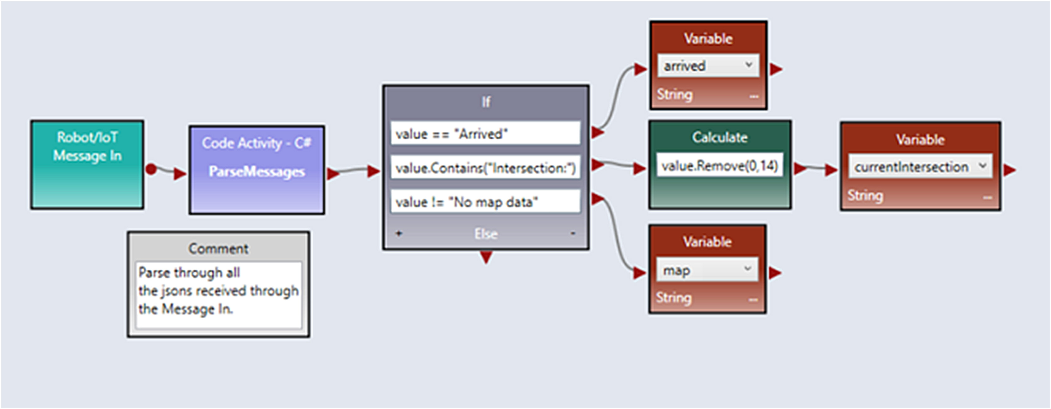
1)RECEIVING MAP INFORMATION FROM THE SIMULATOR
The VIPLE code in Fig. 15 is used to receive the real-time map information from the traffic simulator. As shown in Fig. 12, the JSON structure received from the traffic simulator includes information such as the edges, nodes, and position, each of which are static at every intersection. Additionally, the variable Weight changes over time because the weight takes distance and number of cars between two points into consideration.
2)RECEIVE STARTING POSITION FROM THE SIMULATOR AND DESTINATION FROM USER INPUT
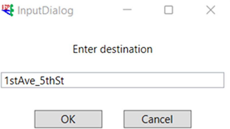
The VIPLE program for this part is presented in Fig. 16. To receive the intersection where the red car is currently located, {“getintersection”: “true”} is used to request the JSON information from the simulator. When the value has been received, it is stored in the source variable which represents the current intersection of the red car. Simple Dialog enables interaction from the user so they can enter the desired destination of the red car as shown in Fig. 17, then it stores it in the variable destination.
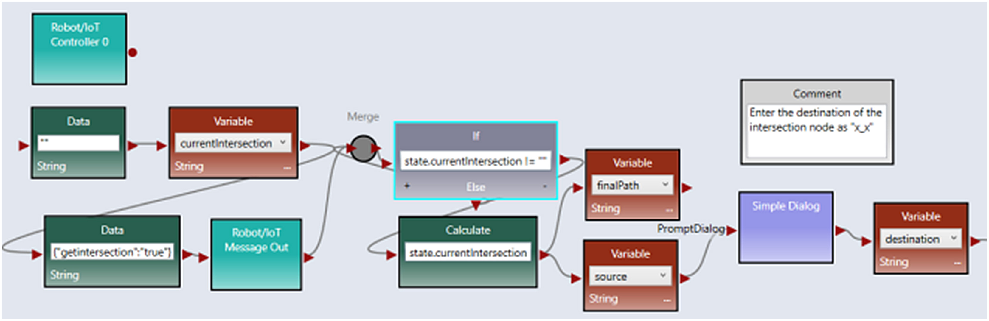 Fig. 16. VIPLE program for Starting Position and Destination.
3)WHILE LOOP CALCULATING THE TRAFFIC AT EACH INTERSECTION
A while loop is used in the program to loop through all the intersections from the starting position of the red car to its destination. At every intersection, the program receives the up-to-date map information and the current intersection. Then, the program uses the new data in the Dijkstra’s algorithm code to calculate a path with the current shortest distance and least traffic. This while loop is a key step to achieving the dynamic goal of the program. The basic structure is shown in Fig. 18.
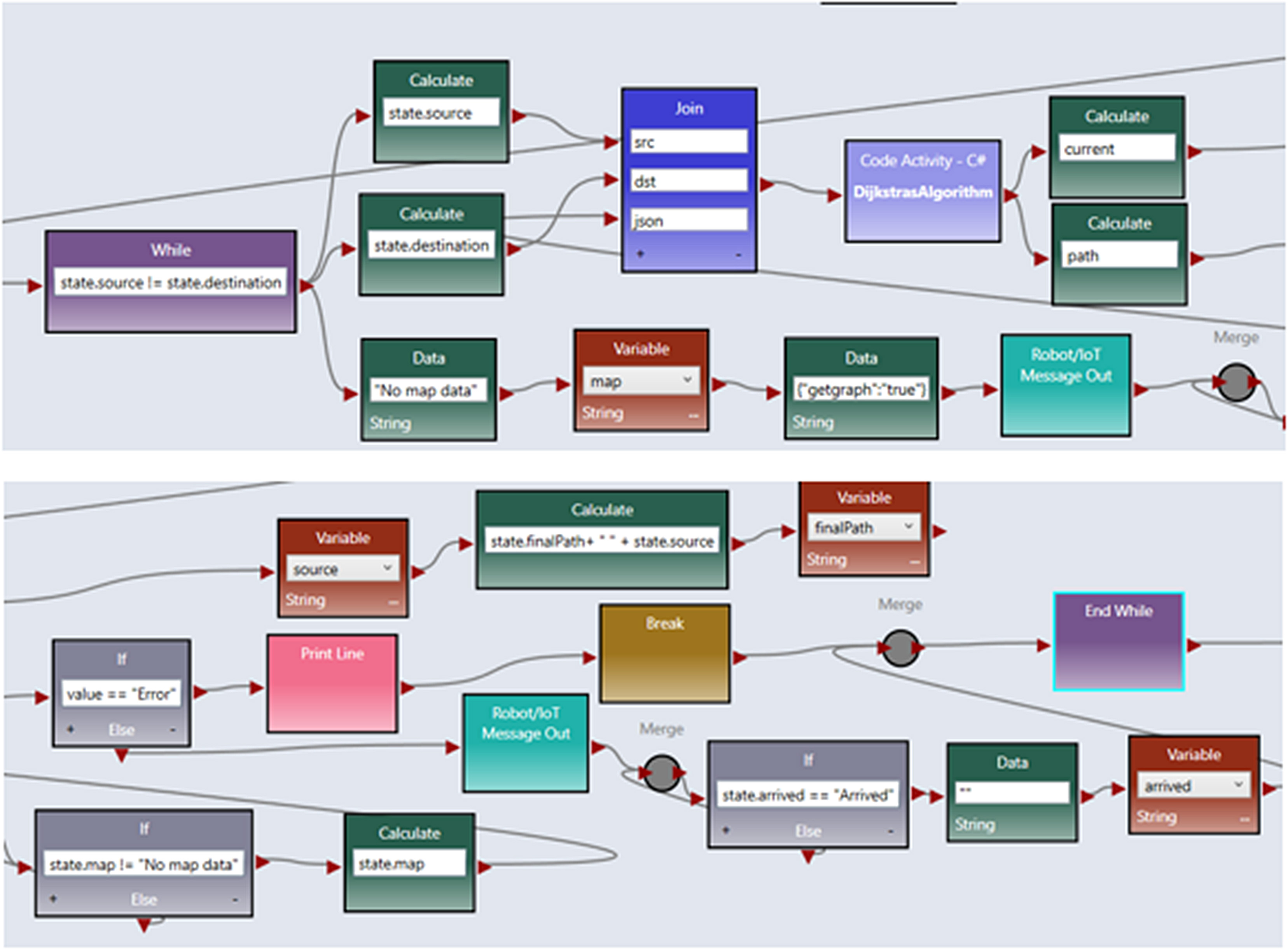
4)DIJKSTRA’S SHORTEST DISTANCE ALGORITHM
Dijkstra’s algorithm, an algorithm to compute the shortest path based on a graph’s edge weights, is implemented as a C# Code Activity in VIPLE. A min-heap is used as the data structure to store nodes, edges, weight, and the adjacency list information. The output of this C# code activity is stored in two variables. The first is the next intersection the red car will be at, which is output as current, then stored in variable source. The second one is output in path, which is the global path to the destination that Dijkstra’s algorithm determined at the current intersection. As shown in Fig. 18, src, dst, and json are the inputs for Dijkstra’s algorithm where src is the current intersection, dst is the destination intersection, and json is the JSON message that is received from the simulator at the current intersection. All three parts of the input are important parameters to be passed into the algorithm.
V.RESULTS AND DISCUSSION
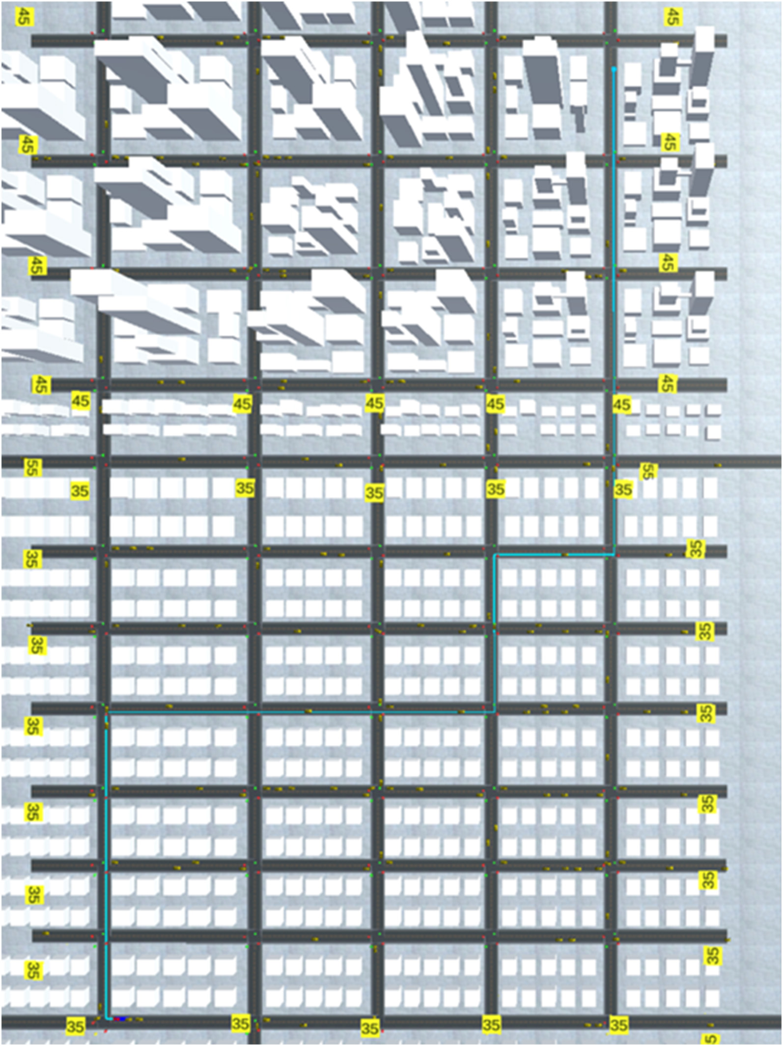
This section presents the output of the implementation of Dijkstra’s algorithm in VIPLE, and the corresponding routes shown in the traffic simulator. Figs. 19–21 are the outputs for the traffic pattern received from the simulator between 7:00 and 8:00. Figure 19shows the printed output of the planned global path at each intersection and the path the red car has taken. In particular, Fig. 19 highlights that the globally best path may change any number of times during execution due to changes in the traffic. The light blue path shown in Fig. 20 is the current planned global path. The dark blue path in Fig. 21 is the path that was actually taken by the red car to arrive at the destination, a history of where the car has traveled based on the dynamically updated global paths. The dark blue path corresponds to the printed output “THE PATH RED CAR HAS TAKEN” in Fig. 19.
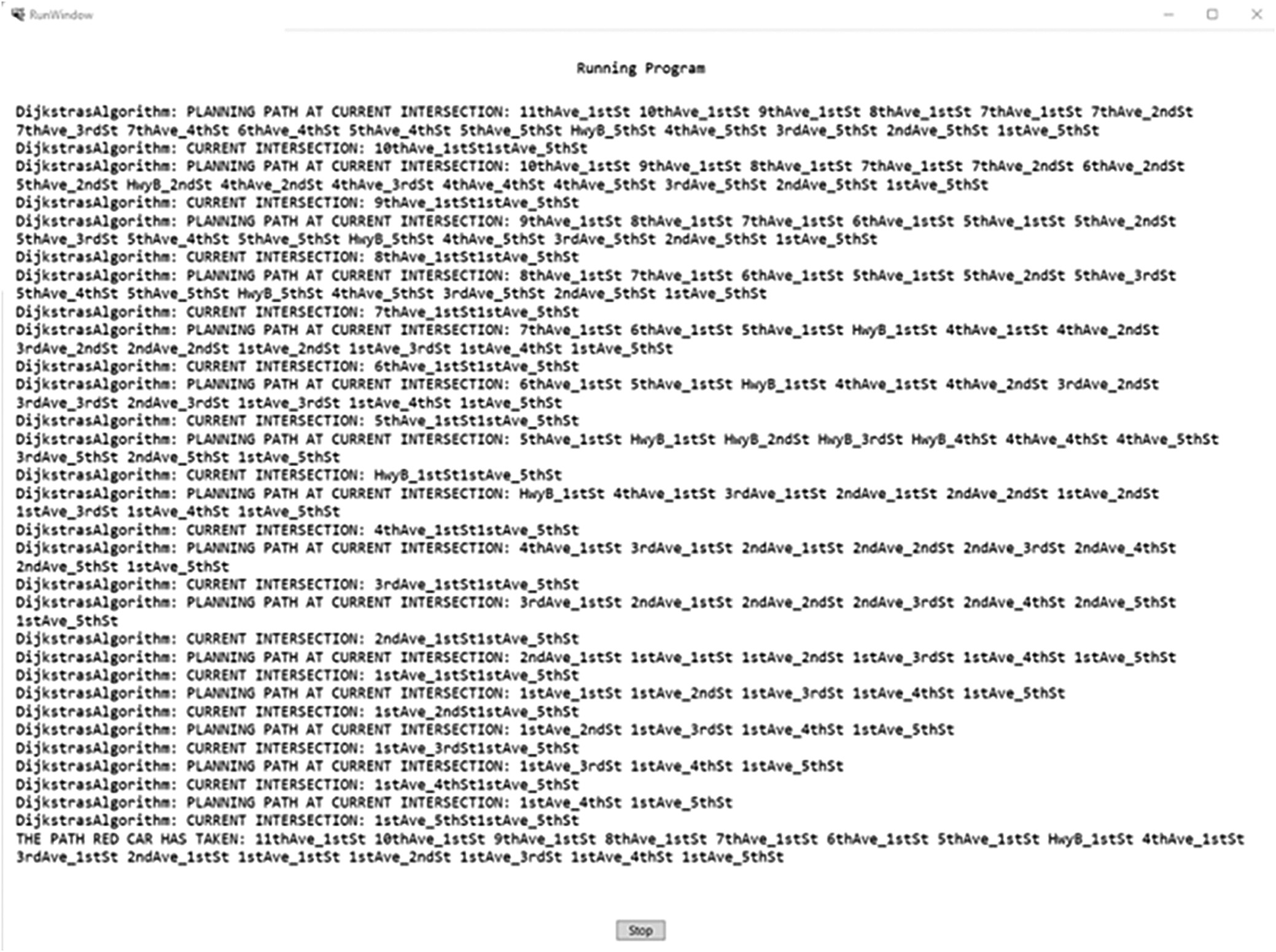 Fig. 19. Printed Output of the Dynamic Dijkstra’s Algorithm.
VI.CONCLUSIONS AND FUTURE WORK
This paper presented a combination of generation of complete datasets from real traffic data, application of this traffic data in the traffic simulator, and dynamic routing algorithms using the generated traffic data. The generation of traffic data was based on real Maricopa County traffic data recorded in 2020. The hourly data for each road were translated manually. Then, the generated data were incorporated into the traffic simulator developed in the Unity game engine. Finally, routing algorithms were implemented in VIPLE by using the dynamically changing traffic data in the simulator to update the red car’s path. This work utilized the VIPLE traffic simulator. Furthermore, this work provided a visualization sample of dynamic routing algorithms for computer science education.
As discussed, real traffic generation in this work can be further improved in future projects. This part can be accomplished by collecting additional traffic data and applying more advanced ML techniques. One example of future research is to train a ML model to predict traffic on each road segment at certain times of the day based on the direction and distance from various city landmarks or popular areas, such as downtown buildings such as skyscrapers, amusement parks, and sports stadiums. Additionally, the same or a different model could be trained to incorporate automobile collisions, perhaps from a dataset with locations of the accident (such as on a freeway or a side street) or with traffic density. Then, the simulator could be updated to have car accidents occur, stalling traffic. These new traffic jams could then be used to verify the existing implementation of Dijkstra’s algorithm and provide grounds for further research into more efficient dynamic path planning algorithms. For the traffic simulator, new functionalities can be incorporated to better simulate real traffic behavior and to show them on the map in real time to depict trends more accurately.
For a self-sustaining approach that uses present day data, an online ML application can be developed that automatically retrieves data from the traffic data website. Such an approach enables verification of student approaches using a variety of datasets and offers the possibility of performing research on modern traffic trends. For example, modern data can be analyzed to determine value of infrastructure changes.