I.INTRODUCTION
The rapid growth of location-acquisition technologies, particularly Global Positioning System (GPS) sensors embedded in mobile devices, has led to an unprecedented growth in the availability of human mobility trajectories. Location-based technology continuously generates extensive spatio-temporal data that capture detailed sequences of movement, providing valuable insights for governments [1–6], urban planners [7–9], technology companies [10–12], researchers [13,14], and particularly intelligent transportation services [15,16]. In large metropolitan areas, ride-hailing platforms like Uber, Grab, Gojek, and Maxim have emerged as key players in the urban mobility ecosystem, significantly altering the landscape alongside conventional public transportation [17–20]. These platforms record every trip, from origin to destination, including the mode of the trip, using GPS and other sensors, and generate comprehensive trajectory data, which includes latitude, longitude, timestamps, and metadata related to trip conditions. Such data streams serve as a crucial foundation for predictive analytics, facilitating next-location prediction [21–25], route forecasting [26,27], traffic management optimization (including forecasting congestion and incidents) [28–30], Personalized Travel Recommendations, and demand estimation [31].
In Indonesia, the recently released Grab-Posisi GPS Trajectory Dataset represents the first large-scale mobility dataset in Southeast Asia, providing a unique opportunity for spatio-temporal research [12,32]. The Grab-Posisi is characterized by high volume and high velocity, making it a valuable asset for developing next-location prediction models, optimizing pick-up and drop-off recommendations and improving real-time mobility services. In addition, the dataset contains exceptionally dense trajectories, with a minimum sampling interval of 1 second and an average interval of 13 seconds, enabling fine-grained modeling of short-term mobility dynamics. Each transportation track is also enriched with contextual metadata, including speed, heading, smartphone operating system, and transportation mode, thereby enhancing the semantic interpretability of movement behavior. Furthermore, the dataset’s broad spatial coverage across Jakarta enables the discovery of various mobility patterns in the city, ensuring a comprehensive understanding of the data, which is vital for developing powerful, generalizable deep learning predictive models. This, in turn, inspires the next wave of innovation in intelligent mobility services.
Spatio-temporal prediction aims to estimate future mobility states from historical movement patterns and contextual information. Accurate next-location prediction plays a critical role in intelligent transportation systems, ride-hailing services, traffic management, and location-aware recommendation systems. Despite the rapid growth of ride-hailing platforms in Indonesia, research on next-location prediction using large-scale Indonesian trajectory datasets remains limited. Existing studies have predominantly focused on datasets collected in North America, Europe, and China, leaving Southeast Asian mobility patterns largely unexplored. This gap is particularly important because mobility behavior is highly influenced by local geographic, socioeconomic, and transportation characteristics.
Although significant progress has been achieved in mobility prediction, existing approaches face several limitations. Many studies rely on sparse trajectory datasets that cannot capture fine-grained mobility dynamics. Furthermore, most prediction models primarily utilize spatial coordinates and temporal sequences while overlooking contextual semantics such as land-use characteristics, neighborhood-level geographic information, and temporal behavioral factors. Third, although recent attention-based, graph-based, and large language model approaches have demonstrated promising performance, comprehensive evaluations on large-scale, dense real-world trajectory datasets remain limited, particularly in Southeast Asia and Indonesia. Consequently, current approaches often struggle to capture the complex interactions between spatial, temporal, and contextual factors that govern human mobility.
To address these limitations, this study proposes a Spatio-Temporal Context Long Short-Term Memory (STC-LSTM) framework that explicitly integrates contextual information into next-location prediction. The framework enriches dense mobility trajectories with temporal and spatial semantic information, including holiday indicators, day-of-week attributes, land-use categories, and postal codes, enabling a more comprehensive representation of mobility behavior. The main contributions of this study are as follows:
- 1.We propose STC-LSTM, a context-aware deep learning framework that jointly models spatial, temporal, and semantic information for next-location prediction.
- 2.We develop a semantic enrichment pipeline that integrates temporal annotations, land-use information, postal codes, map-matched trajectories, and contextual embeddings into dense mobility representations.
- 3.We conduct a comprehensive evaluation on the Grab-Posisi dataset, comprising approximately 56,000 trajectories and 5.6 million GPS points, to quantify the contribution of different contextual factors to prediction performance.
- 4.We demonstrate that contextual enrichment substantially improves prediction performance, reducing prediction error by up to 75% compared with trajectory-only baselines.
The remainder of this paper is organized as follows. Section II reviews the existing literature on mobility prediction, including traditional statistical approaches, deep learning-based methods, context-aware mobility modeling, and the research gaps that motivate this study. Section III presents the proposed methodology, including data preparation, semantic trajectory enrichment, map-matching, and the development of the STC-LSTM model. Section IV describes the experimental set-up and presents results across different contextual configurations, highlighting the impact of semantic and temporal information on next-location prediction performance. Finally, Section V concludes the paper by summarizing the main findings, contributions, limitations, and directions for future research.
II.LITERATURE REVIEW
Human mobility prediction has become an important research topic in intelligent transportation systems, location-based services, and urban analytics. Early studies primarily employed statistical and probabilistic approaches, such as Markov Chains, Hidden Markov Models (HMMs), and Bayesian frameworks, to model sequential movement behavior from GPS trajectories. Zong et al. [33] developed destination-prediction models based on multi-day GPS trajectories using a combination of Markov Chains, Multinomial Logit models, and HMMs. Similarly, Wang et al. [34] proposed a mobility prediction framework based on a Bayesian mixture model and hierarchical Dirichlet process to address sparse trajectory data. While these methods successfully captured mobility regularities, they generally relied on limited contextual information and could not represent complex nonlinear movement patterns, particularly when dealing with large-scale, highly dynamic trajectory datasets.
Deep learning has significantly advanced next-location prediction by enabling the modeling of complex spatial–temporal dependencies in mobility trajectories. LSTM networks have been widely adopted for their ability to capture long-term sequential patterns, and studies have demonstrated that incorporating auxiliary information, such as travel time, can further improve prediction accuracy [35]. Beyond recurrent architectures, attention-based models such as the Spatio-Temporal Attention Network (STAN) have enhanced prediction robustness by learning explicit spatial and temporal correlations within trajectories and capturing relationships between non-adjacent locations and non-consecutive visits [21]. More recently, graph-based and attention-driven approaches have been introduced to model mobility preferences and contextual interactions, leveraging graph representations and real-world mobility information to improve destination and next-location prediction performance [22,36]. These developments highlight the effectiveness of deep learning for mobility prediction while demonstrating the growing importance of richer spatial-temporal.
Context-aware mobility modeling has emerged as a promising approach to address the limitations of trajectory-only prediction by enriching mobility data with temporal and spatial semantics, such as holidays, day-of-week information, land-use characteristics, and neighborhood attributes. By incorporating contextual information, these approaches aim to better capture the environmental and behavioral factors that influence human mobility [22,24,36]. However, existing studies typically utilize only a limited set of contextual features or evaluate their methods on relatively sparse trajectory datasets [24,35]. Moreover, research investigating large-scale context-aware mobility prediction using dense real-world trajectories, particularly in Southeast Asia, remains limited. These challenges highlight the need for more comprehensive frameworks capable of jointly modeling spatial, temporal, and semantic information for next-location prediction.
Overall, the literature demonstrates a clear evolution from statistical and probabilistic approaches toward deep learning and context-aware mobility prediction models. While recent studies have improved the ability to capture spatial–temporal dependencies and contextual interactions, important challenges remain. Existing methods often rely on sparse trajectory datasets, utilize only a limited set of contextual features, or lack evaluation on large-scale dense real-world mobility data. Furthermore, the joint integration of multiple contextual dimensions, including temporal, geographic, and semantic information, remains relatively underexplored. These limitations motivate the development of a more comprehensive framework capable of jointly modeling spatial, temporal, and contextual factors to improve next-location prediction performance.
III.METHOD
This section describes a methodological framework for constructing high-quality, semantically enriched spatio-temporal trajectories for next-location prediction.
A.DATA PREPARATION
The data preparation workflow consists of four key components: data cleaning, trajectory generation, semantic annotation, and spatial smoothing, all of which support the development of deep learning models, as illustrated in Fig. 1. This comprehensive pipeline aims to inspire researchers and data scientists to adopt and adapt the approach confidently in their own work.
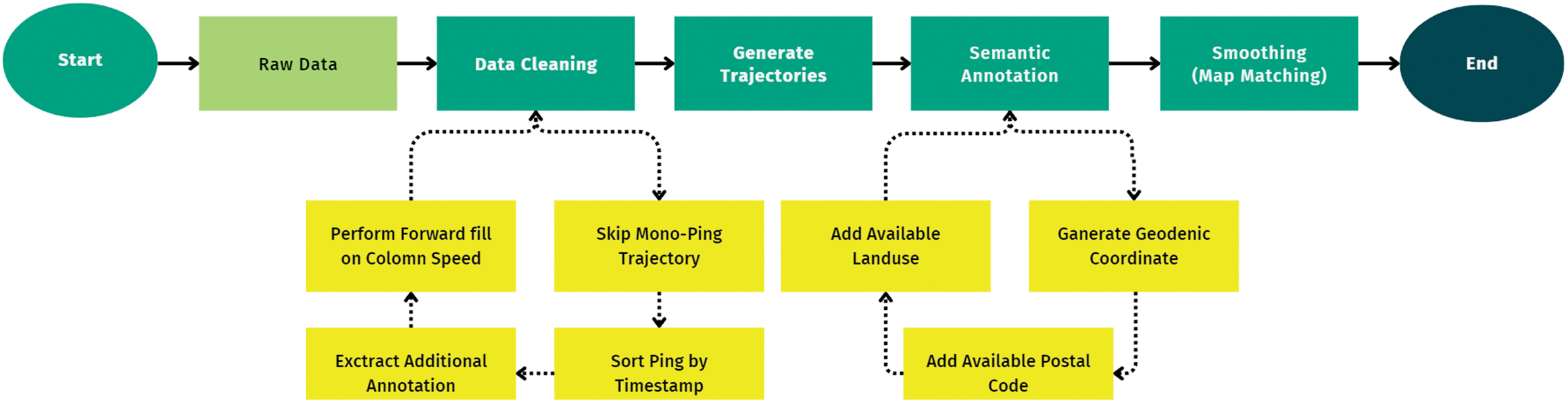 Fig. 1. Proposed context-enriched trajectory preparation pipeline for STC-LSTM-based next-location prediction.
First, raw trajectory data undergo a data cleaning procedure that includes forward-filling missing speed values, removing monopings, sorting pings by timestamp, and extracting additional available metadata to ensure temporal consistency (such as day_of_week and is_holiday) and structural completeness. We grouped the data by “trj_id” to ensure each group had a complete trajectory, serving as a representation. Second, the cleaned data is transformed into ordered movement sequences through a trajectory-generation step that reconstructs user mobility paths. Third, a semantic-annotation module enriches each trajectory point with contextual attributes by integrating available land-use information, postal codes, and geodesic coordinates, thereby producing trajectories with both geometric and semantic depth. Finally, a smoothing stage employing map-matching techniques aligns the annotated trajectories to the underlying road network to reduce GPS noise and ensure spatial accuracy. These four stages collectively produce high-quality, semantically enriched spatio-temporal trajectories suitable for downstream modeling and prediction tasks.
During the data preparation phase, a series of critical steps are taken to ensure the data is clean and ready for further analysis. The raw data used are from Grab-Posisi, the first GPS trajectory dataset in Southeast Asia, encompassing both developed countries, such as Singapore and Indonesia [32]. The dataset’s large volume, with 56,000 trajectories and 5.6 million GPS pings, demonstrates its richness and potential for detailed analysis. Each ping contains a trajectory ID, latitude, longitude, timestamp (UTC), accuracy level, bearing, and speed, as illustrated in Fig. 2. The minimum GPS sampling rate is 1 second, with an average of 13 seconds, the highest among existing open-source datasets, indicating a high frequency of data capture and providing detailed and accurate information about user movements.
 Fig. 2. Sample trajectory records and metadata attributes in the Grab-Posisi dataset.
1).DATA CLEANING & SEMANTIC ANNOTATION
The raw dataset, provided in Parquet format (Fig. 2), requires substantial preprocessing to standardize and simplify its structure. Trajectory identifiers (trj_id) and point identifiers (point_id) are converted into sequential numeric indices and regrouped to ensure consistent ordering. During this phase, several data inconsistencies are identified, including negative speed values and single-point trajectories, neither of which represents meaningful movement and therefore holds little analytical value. As a result, these invalid records are removed from the dataset. In total, 8.879 points across 3.617 trajectories contained negative speed values, indicating potential measurement errors or sensor anomalies. To mitigate their impact, a forward-fill strategy is applied, replacing invalid entries with the most recent valid observation. This procedure improves dataset coherence and minimizes distortions or biases caused by unrealistic speed measurements.
Semantic context annotations are categorized into temporal attributes (day_of_week, is_holiday) and spatial attributes (latitude, longitude, land use, and postal code). Temporal semantics are derived directly from the timestamp, where the day_of_week feature distinguishes weekdays from weekends, and is_holiday is determined by importing the Python holidays module and creating a list of public holidays for Indonesia using the “holidays.CountryHoliday('ID')” function. This function checks whether a given date is in the holidays list and returns True if it is and False otherwise. The result is stored in a newly defined field “is_holiday.” This method ensures that each record in the dataset includes a Boolean indicator specifying whether the associated date is a public holiday in Indonesia. Furthermore, a function determine_day_of_week(date) is defined to specify the day type based on the given date. The function first converts the date to the name of the day using format_date_to_day_name(date). If the resulting day name is “Saturday” or “Sunday,” the function returns “Weekend”; otherwise, it returns “Weekday.” Subsequently, each record in the dataset is processed to classify the started_at date.
Figure 3 illustrates the statistics of the Grab-Posisi data after deriving the temporal additional features. The Grab demand in Jakarta transportation services begins at 6 AM, reaching its peak at 10 AM. Conversely, the period from 5 PM to 9 PM is the least busy. It also reveals that the number of trips on weekdays exceeds that on weekends, with a substantial disparity. Additionally, a similar pattern is observed between holidays and non-holidays, with a more pronounced difference indicating significantly fewer trips on holidays than on regular days.
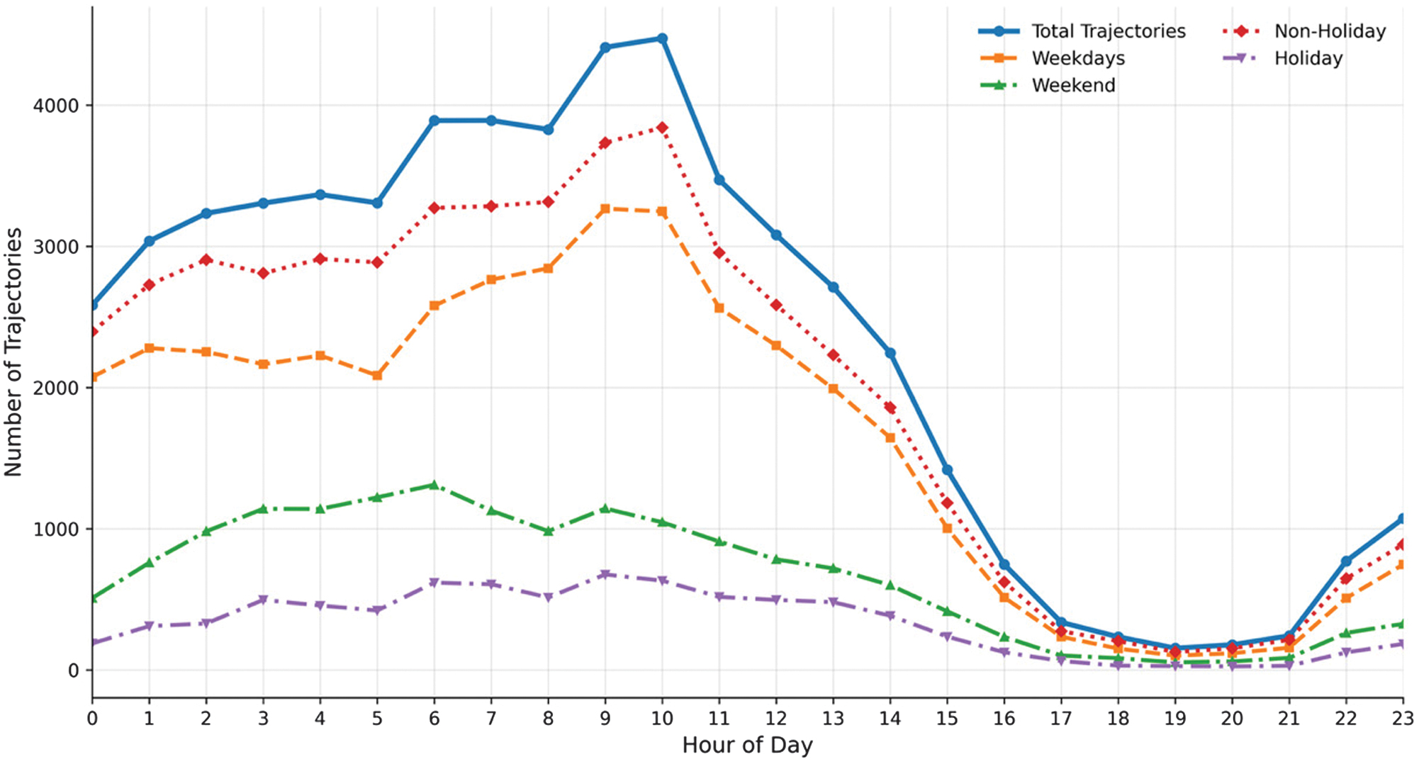 Fig. 3. Temporal distribution of mobility trajectories by hour, day type, and holiday status.
Spatial semantics are generated by mapping the trajectories (origin and destination) into the OpenStreetMap database for Indonesia, which provides standardized land-use classifications and postal code information [37]. Algorithm 1 outlines the procedure for generating the land-use context.
Algorithm 1. Land-use context extraction based on openstreetmap
| lat_lon_to_landuse ← create dictionary from CSV (latitude, longitude) to landuse |
| connect to PostgreSQL and fetch all points (point_id, lat, lon) |
| for each (point_id, lat, lon) in fetched points do |
| if (lat, lon) in lat_lon_to_landuse then |
| landuse ← lat_lon_to_landuse[(lat, lon)] |
| else |
| nearest_point, nearest_dist ← None, ∞ |
| for each (x, y) in lat_lon_to_landuse.keys() do |
| tmp_dist ← geodesic((lat, lon), (y, x)).km |
| if tmp_dist < nearest_dist then |
| nearest_dist, nearest_point ← tmp_dist, (x, y) |
| landuse ← lat_lon_to_landuse[nearest_point] |
| write update query to file with point_id and landuse |
| reconnect to PostgreSQL and execute queries from file |
| commit changes and close connection |
The “get_landuse()” function extracts land-use data by reading the geospatial file to identify the land-use geometric types of origin and destination points of trajectories. We perform spatial operations to determine if the origin or destination is within the polygon in the database. If it is within the polygon, retrieve the polygon’s land use. If not, then use the Vincenty (geodesic) method to get the nearest land-use polygon by calculating the shortest distance between points and polygons. The nearest land-use value is then updated in the database for each point. The Vincenty method is a widely used geodesic algorithm for calculating the shortest distance between two points on the Earth’s surface, taking into account the planet’s ellipsoidal shape. It is an iterative method renowned for its high accuracy in calculating distances on the ellipsoid, making it a preferred choice for geospatial analyses.
Figure 4 shows that the majority of trips occur within residential areas, which dominate the distribution by a substantial margin, followed by military zones as the second-most-frequent land-use category. The remaining classes: brownfield, cemetery, grass, and retail appear with considerably lower and relatively comparable frequencies. The temporal distribution also aligns with the trend observed in Fig. 3, with trip activity concentrated between 06:00 and 12:00, peaking around 10:00–11:00 before steadily declining through 19:00.
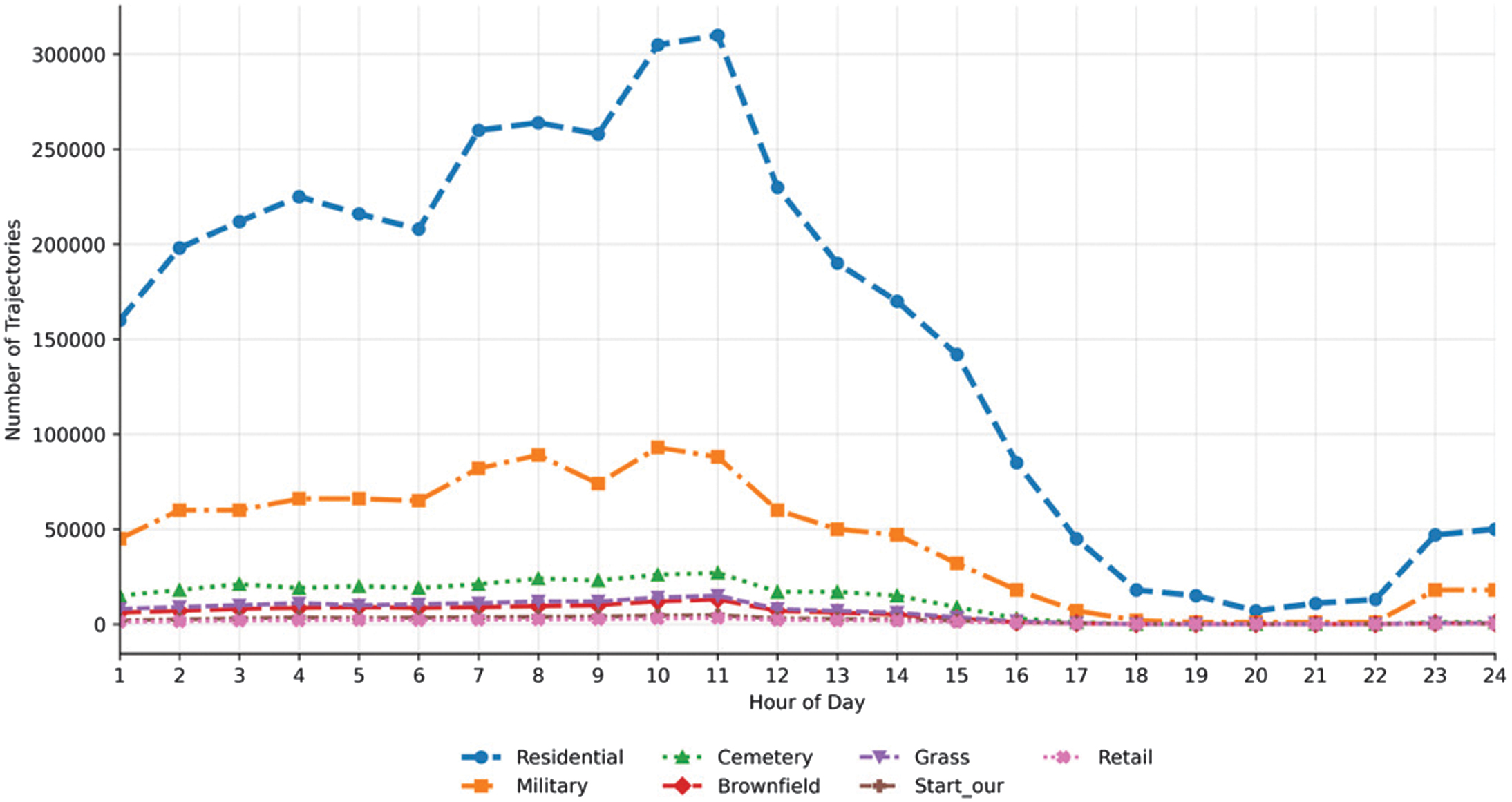 Fig. 4. Hourly distribution of trajectories across different land-use categories.
Incorporating postal codes enriches each trajectory with fine-grained spatial semantics, enabling the model to capture neighborhood-level movement patterns that are otherwise indistinguishable in raw coordinate data. This additional contextual layer enhances the model’s interpretability and predictive capabilities by linking mobility behavior to underlying socio-geographical structures. The dataset comprises over 407 unique postal codes and six land-use types, enriching the data with contextual information to improve prediction performance.
Algorithm 2 first constructs a dictionary from a CSV file, where each latitude–longitude pair is associated with its corresponding postal code. Using the coordinate keys from this dictionary, a cKDTree structure is then generated to support efficient nearest-neighbor searches. When processing each trajectory point retrieved from the PostgreSQL database, the algorithm first attempts a direct dictionary lookup for the postal code; if the point’s coordinates are not present in the dictionary, it then queries the cKDTree to find the nearest coordinate. Postal codes identified through either method are compiled into update statements, which are executed in batches of 1,000 records to optimize database performance. Once all updates are applied, the database connection is closed.
Algorithm 2. Postal Code Extraction
| create lat_lon_to_postalcode dictionary from CSV |
| build cKDTree from lat_lon_to_postalcode keys |
| connect to PostgreSQL and fetch points (point_id, lat, lon) |
| for each point (point_id, lat, lon) do |
| postalcode ← lat_lon_to_postalcode.get((lat, lon)) |
| if postalcode is None then |
| nearest_point ← tree.query([lat, lon]) |
| postalcode ← lat_lon_to_postalcode[nearest_point] |
| if postalcode is not None then |
| add update query to list |
| batch_size ← 1000 |
| for each batch of update queries do |
| execute and commit batch in PostgreSQL |
| close database connection |
Table I shows the top 10 postal codes ranked by trajectory count, indicating that the distribution of these 10 postcodes is relatively even, given the nearly 5.6 million points. These 10 postcodes are also expected to be prominently represented and distributed across approximately 56,000 recorded trajectory data points.
Table I. Top 10 postal codes areas with the highest number of recorder trajectories
| Postal code | Count |
|---|---|
| 11610 | 74158 |
| 11470 | 71104 |
| 15810 | 67910 |
| 12310 | 64071 |
| 11730 | 62916 |
| 14240 | 61090 |
| 17510 | 60355 |
| 17530 | 59905 |
| 11530 | 55888 |
| 14450 | 48970 |
2).SMOOTHING
During the trajectory data validation stage, several GPS points are identified as deviating from the underlying road network, indicating errors in off-road positioning. Highlighting the importance of accuracy helps the audience trust the data’s reliability. Consequently, a correction procedure, such as map-matching or filtering based on accuracy thresholds, is required to realign these points with the actual road geometry. Positional uncertainty is explicitly captured in the accuracy attribute of the Grab-Posisi dataset, which represents the precision of each recorded GPS observation. This attribute is measured in meters and denotes the radius of a circular confidence area surrounding a GPS point, within which the actual location is expected to lie. Smaller accuracy values indicate higher positional precision, whereas larger values reflect greater uncertainty. As such, the accuracy attribute provides critical information for assessing the reliability of GPS points and serves as an essential indicator for subsequent map-matching and trajectory-smoothing processes.
Specifically, trajectories with trj_id 15096 and 11956 exhibited average positional accuracies of 41.38 m and 35.30 m, respectively, which are close to the overall dataset average (above 30 m) and thus serve as representative cases for baseline evaluation. In contrast, trajectories with trj_id 21873 and 54225 show substantially higher average inaccuracies of 80.60 m and 64.50 m, respectively, indicating more severe deviations from the true road geometry and posing greater challenges for map-matching algorithms.
Including trajectories with both moderate and high positional uncertainty enables a more comprehensive and robust evaluation of map-matching performance. In particular, trajectories 21873 and 54225 contain a large proportion of points located far from the actual road network, providing a stringent test for algorithmic robustness. A map-matching model that performs well across this diverse set of trajectories can therefore be considered reliable for real-world applications involving heterogeneous data quality.
To mitigate GPS noise and correct spatial inconsistencies in the trajectory data, this study adopts a map-matching framework based on the Longest Common Subsequence (LCSS) approach. Four map-matching approaches are comparatively assessed: Euclidean Distance Matrix, Kalman Filter, HMM, and LCSS. The Euclidean Distance Matrix method assigns each GPS point to the nearest road segment independently, disregarding global path continuity, which leads to frequent mismatches and fragmented trajectories. The Kalman Filter reduces random noise but fails to consistently align points with the true road geometry, leading to persistent off-road positioning errors. The HMM improves path alignment by modeling sequential dependencies; however, it produces trajectories that are significantly shortened by approximately 30–65% of the original length, thereby distorting the actual travel path. In contrast, the LCSS-based approach successfully aligns all GPS points with the appropriate road segments, while preserving the overall trajectory length and structural integrity.
Across all evaluated trajectories (15096, 11956, 21873, and 54225), the LCSS-based map-matching model consistently outperforms the alternative methods, as illustrated in Fig. 5. The results demonstrate that LCSS effectively preserves both spatial accuracy and trajectory continuity, even under conditions of high positional noise and dense sampling. Its ability to maintain both spatial correctness and path continuity makes it the most accurate and representative approach for map-matching in the context of high-noise, dense trajectory data and therefore the preferred preprocessing method for subsequent spatio-temporal modeling.
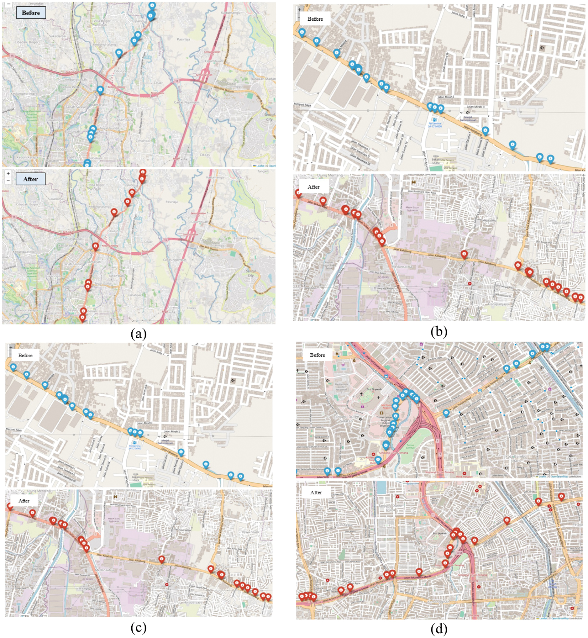 Fig. 5. Representative examples of LCSS-based map-matching before and after trajectory correction. (a) 21873, (b) 54225, (c) 15096, and (d) 11956.
B.BUILDING MODEL
This subsection introduces the proposed LSTM-based modeling framework for next spatio-temporal location prediction. The model is designed to learn sequential mobility patterns from dense, semantically enriched trajectories by jointly capturing temporal dependencies and spatial dynamics embedded in ordered movement sequences. By leveraging the LSTM’s capability to model long-term dependencies in time-series data, the proposed approach effectively integrates historical movement information with contextual features to predict the subsequent location in both spatial and temporal dimensions. The following sections detail the model architecture, input feature representation, and training procedure.
We propose an LSTM-based architecture, termed STC-LSTM, to enhance next spatio-temporal location prediction by jointly modeling spatial, temporal, and contextual information. As illustrated in Fig. 6, the spatial component captures geographic coordinates of trajectory points, the temporal component models time-related factors, and the contextual component incorporates auxiliary semantic attributes, including holidays, day of the week, postal codes, and land-use categories. By integrating these heterogeneous features, STC-LSTM learns a more comprehensive representation of user mobility behavior, enabling the model to capture how environmental and temporal contexts influence movement patterns and, consequently, improve prediction accuracy.
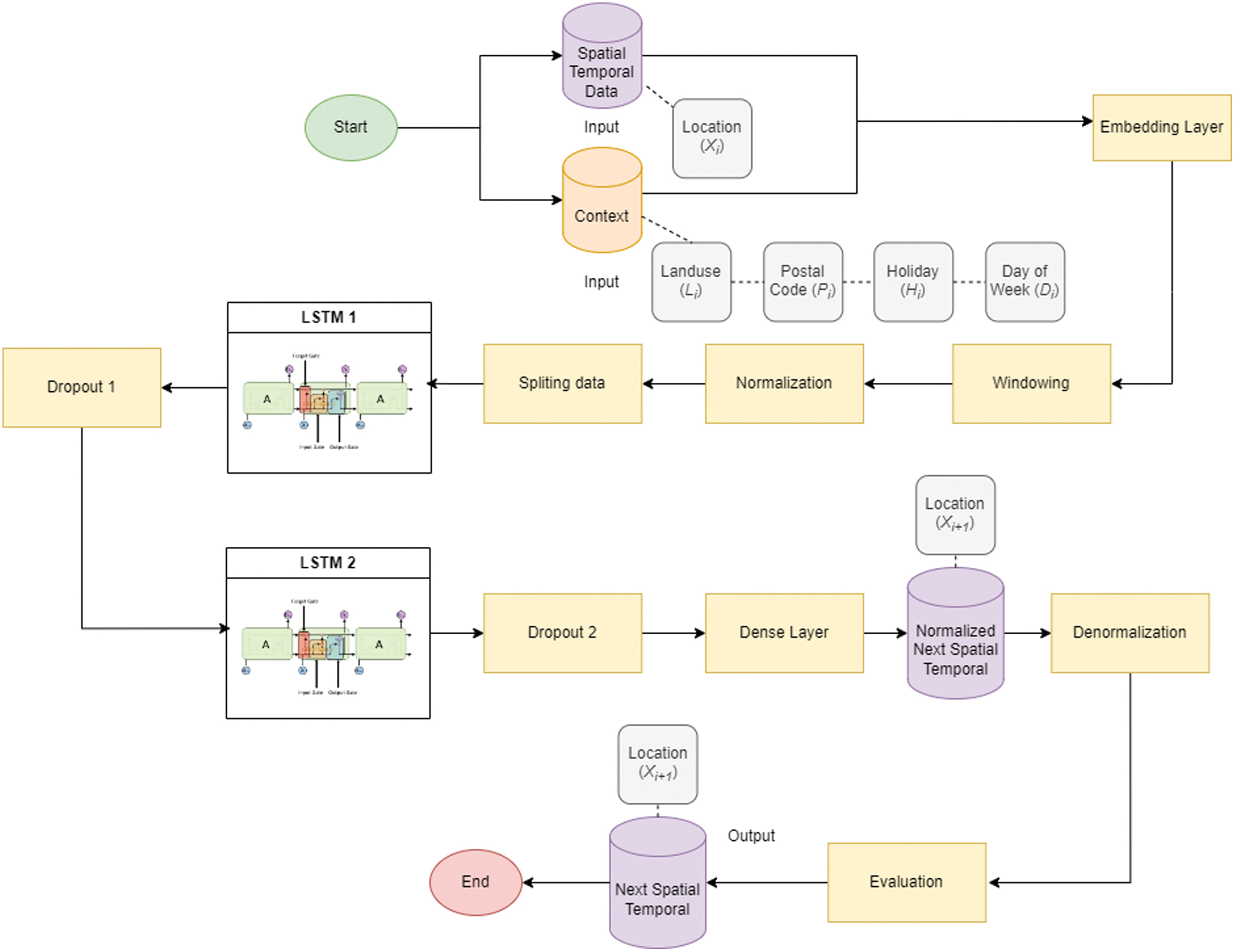 Fig. 6. Proposed context-aware spatio-temporal trajectory prediction framework based on stacked LSTM networks.
The STC-LSTM architecture operates on ordered trajectory sequences, where the index i denotes the current position in a trajectory. The input layer receives spatio-temporal information consisting of the current location (Xi), together with contextual attributes, including land-use type (Li), holiday indicator (Hi), day-of-week label (Di), and postal code (Pi). To effectively represent categorical contextual information, an embedding layer transforms these variables into dense continuous vectors, enabling the model to learn latent semantic relationships among contextual categories. The embedded contextual features are then combined with spatial–temporal trajectory information and organized into fixed-length sequences using a windowing mechanism. Feature normalization is subsequently applied to ensure numerical stability and balanced feature contributions during training.
The resulting sequence representation is processed through two stacked LSTM layers. The first LSTM layer captures local mobility dynamics and short-term movement dependencies, while the second LSTM layer learns higher-level temporal patterns and longer-term behavioral dependencies from the hidden representations generated by the preceding layer. Dropout regularization is incorporated between layers to reduce overfitting and improve model generalization. The final hidden representation is then passed to a fully connected dense layer with ReLU activation to model nonlinear interactions among spatial, temporal, and contextual features. Finally, the output layer predicts the next location (Xi + 1), and the predicted coordinates are denormalized to restore their original scale. This information flow enables STC-LSTM to jointly learn spatial, temporal, and contextual mobility patterns for accurate next-location prediction.
1).MATHEMATICAL FORMULA OF STC-LSTM
The STC-LSTM model predicts the next spatial location by jointly encoding spatial coordinates, temporal signals, and semantic contextual attributes within a gated recurrent architecture. The complete framework is expressed through five consolidated equations below.
Input Representation
At each time step i, the enriched input vector is formed by concatenating continuous features with learned embeddings for the three categorical attributes: day-of-week Di, land use Li, and postal code Pi:
where xi and yi are normalized latitude/longitude, ti is the normalized timestamp, Hi ∈ {0,1} is the binary holiday indicator, and ED, EL, and EP are learnable embedding matrices.LSTM Cell Update
All four gates (forget f, input i, candidate g, output o), the cell state c, and the hidden state h are computed in a single gated cell update. and b_gates stack the four gate weight matrices and biases:
where σ(·) is the sigmoid function, tanh(·) is the hyperbolic tangent, and ⊙ denotes element-wise multiplication.Stacked Layers with DropoutTwo LSTM layers (ℓ = 1, 2) are stacked, where . Dropout is applied after each layer during training to prevent overfitting:Output Prediction and Denormalization
The final hidden state hT(2) is passed through a dense ReLU layer and a linear output head to yield the predicted normalized coordinates , which are then scaled back to geographic coordinates:
where represents the final predicted latitude (equivalently for longitude), and xmax and xmin are the normalization bounds.Training Objective
The model is trained end-to-end by minimizing the mean squared error (MSE) between predicted coordinates and and ground-truth locations over M training windows:
All parameters Θ = {W_gates, W_d, , b_gates, b_d, , ED, EL, EP} are optimized jointly using the Adam optimizer with learning rate η ∈ {0.01, 0.001} and batch size ∈ {128, 512}, as determined by Bayesian hyperparameter search. Training uses a sliding window of size w ∈ {3, 10} to construct input–output pairs from each trajectory.
IV.RESULTS AND DISCUSSION
This section presents and analyzes the experimental results obtained from the proposed STC-LSTM framework for next spatio-temporal location prediction. We first report the quantitative performance of the model under different experimental settings and compare it with baseline approaches to evaluate prediction accuracy and robustness. The results are then discussed in depth to highlight the impact of dense trajectory data and contextual enrichment on model performance and to provide insights into the strengths and limitations of the proposed approach in real-world mobility prediction scenarios.
A.EXPERIMENT SCENARIO
Figure 7 illustrates the experimental design adopted to assess the effectiveness of the proposed STC-LSTM framework for next spatio-temporal location prediction under varying contextual configurations. To systematically evaluate the contribution of contextual information, a series of controlled experiments is conducted in which different combinations of spatial, temporal, and semantic features are incorporated into the model. The objective of these experiments is to quantify how individual contextual factors, as well as their joint integration, influence prediction accuracy, as measured by the MSE and mean absolute error (MAE) metrics.
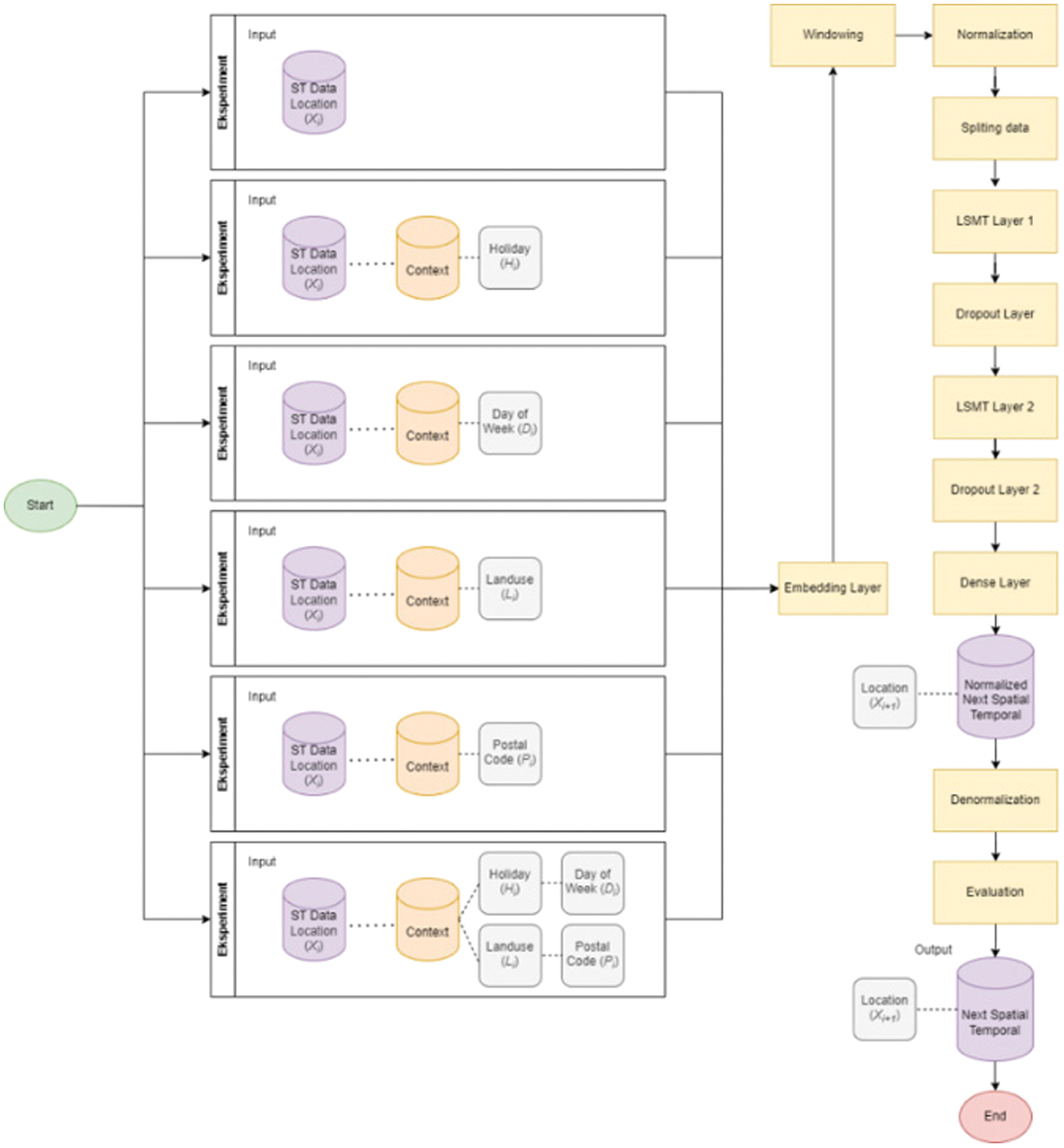 Fig. 7. Experimental configurations of the STC-LSTM framework for contextual-aware next-location prediction.
The experimental scenarios are structured as follows:
- 1.No Context (Baseline): This experiment serves as the baseline configuration, where the STC-LSTM model utilizes only spatial–temporal trajectory information (location and time) without any additional contextual features. Establishing this baseline is crucial for a fair comparison, and we want to reassure that this approach provides a solid reference point to measure the impact of added contextual features.
- 2.Is_holiday context: In this scenario, a binary holiday indicator (is_holiday) is incorporated into the model to capture variations in mobility behavior on public holidays. This experiment assesses the impact of holiday-related temporal context on movement patterns and prediction performance.
- 3.Day_of_week context: This experiment introduces the day_of_week feature, allowing the model to learn weekly mobility regularities, such as differences between weekdays and weekends. The aim is to assess whether recurring weekly patterns improve the accuracy of predictions of the next location.
- 4.Land-use context: Land-use information is added to represent the functional characteristics of locations (e.g., residential, commercial, industrial). This experiment examines how semantic knowledge of the surrounding environment influences spatial transition behavior.
- 5.Postal code context: This scenario augments the model with postal code information, providing fine-grained geographic context at the neighborhood level. The objective is to evaluate whether localized spatial semantics improve the model’s ability to predict subsequent movements.
- 6.All contexts combined (is_holiday, day_of_week, landuse, and postal code): The final experiment integrates all available contextual features simultaneously. This comprehensive configuration assesses the cumulative effect of full contextual enrichment on prediction accuracy, representing the complete STC-LSTM framework.
Across all scenarios, the contextual features are embedded and processed through the same STC-LSTM architecture, including windowing, normalization, stacked LSTM layers, and dense output layers, ensuring a fair comparison. We have designed this methodology to be transparent and reproducible, aiming to build confidence in the robustness of our evaluation. By progressively enriching the input with semantic context, these experiments provide insight into the relative and combined contributions of temporal and spatial semantics to next spatio-temporal location prediction.
To identify optimal model configurations for spatio-temporal prediction, this study employs Bayesian Optimization implemented via the Optuna framework. Bayesian Optimization is selected for its efficiency in navigating high-dimensional, non-convex hyperparameter spaces, particularly for deep learning models where exhaustive grid search becomes computationally infeasible. By iteratively modeling the relationship between hyperparameters and objective performance, Bayesian Optimization enables informed exploration and exploitation of promising regions in the search space.
In this study, Optuna is used to fine-tune key hyperparameters of the proposed STC-LSTM models under various contextual settings, including configurations with and without semantic enrichment. The optimization process evaluates multiple combinations of architectural and training hyperparameters, as summarized in Table II, including the number of LSTM units per layer, dropout rates, learning rate, batch size, and window size. Each candidate configuration is trained and evaluated using the same experimental protocol, with Test MSE and MAE serving as the objective function. To ensure fairness and reproducibility, the best-performing hyperparameter set identified through Bayesian Optimization is consistently applied across all prediction experiments.
Table II. Hyperparameter configurations evaluated in the STC-LSTM experiments
| Hyperparameter | Value 1 | Value 2 |
|---|---|---|
| lstm_units1 | 64 | 128 |
| dropout_rate1 | 0,1 | 0,2 |
| lstm_units2 | 16 | 32 |
| dropout_rate2 | 0,2 | 0,5 |
| learning_rate | 0,01 | 0,001 |
| batch_size | 128 | 512 |
| window size | 3 | 10 |
| optimizer | adam | |
| epoch | 20 | |
The results indicate that the fully context-enriched configuration, incorporating is_holiday, day_of_week, land-use, and postal code features, achieves the best predictive performance. This configuration yields the lowest Test MSE of 1.04 × 10⁻⁵, demonstrating the effectiveness of combining contextual information with optimized model settings. The optimal hyperparameter configuration consisted of moderate LSTM capacities (64 units in the first layer and 32 units in the second layer), dropout rates of 0.2 for both layers, a learning rate of 0.01, and a batch size of 512. This combination provides a balanced trade-off between model expressiveness and regularization, effectively mitigating overfitting while maintaining stable and efficient convergence during training. Given its consistent superiority over alternative configurations, this hyperparameter set is adopted as the benchmark setting for STC-LSTM prediction experiments.
B.RESULTS
This subsection presents the experimental results obtained from the proposed STC-LSTM framework and analyzes the impact of contextual enrichment on next spatio-temporal location prediction performance across different experimental configurations.
Figure 8 illustrates the convergence behavior and predictive performance of the proposed STC-LSTM model under different contextual configurations across training epochs, evaluated using MSE and MAE. The results are reported for two temporal window sizes (3 and 10) and compare six experimental settings: without context (baseline), individual contextual features (is_holiday, day_of_week, landuse, and postalcode), and the complete contextual configuration integrating all features.
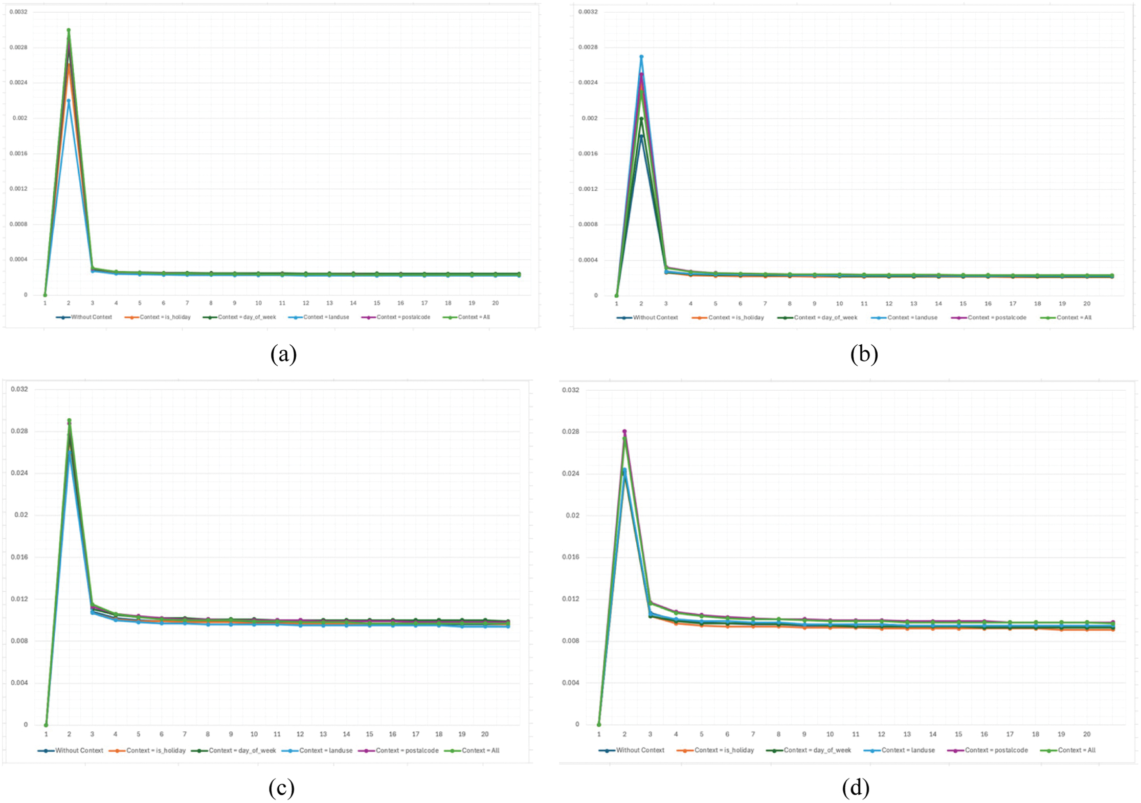 Fig. 8. Training convergence and prediction error comparison of STC-LSTM under different contextual configurations and window sizes. (a) MSE, window size = 3; (b) MSE, window size = 10; (c) MAE, window size = 3; (d) MAE, window size = 10.
Across all scenarios, a sharp reduction in error is observed during the early epochs, indicating rapid learning and stable convergence of the LSTM-based models. After approximately three epochs, both MSE and MAE gradually decrease and stabilize, demonstrating consistent optimization behavior across different context settings. Notably, models incorporating contextual information consistently outperform the baseline configuration without context, achieving lower error values throughout training.
Among individual contextual features, day_of_week, landuse, and postalcode yield more pronounced improvements than is_holiday, highlighting their significant role in improving prediction accuracy. This demonstrates that recurring temporal patterns and fine-grained spatial semantics are particularly valuable, validating their importance in model design. The full context configuration achieves the best overall performance, consistently yielding the lowest MSE and MAE values across both window sizes. This confirms that jointly modeling temporal, spatial, and semantic context enables the STC-LSTM framework to capture complex mobility dynamics more effectively than relying solely on spatio-temporal information. Furthermore, a larger window size (10) generally yields marginally better performance than a smaller one (3), suggesting that incorporating longer historical trajectories improves the model’s ability to learn long-term dependencies in movement behavior.
After training, we evaluate the STC-LSTM’s predictive performance on the test dataset across different contextual configurations, using MSE as the evaluation metric. We also measure the percentage improvement in prediction accuracy relative to the baseline model to quantify the effectiveness of each contextual configuration. The improvement is computed based on the reduction in MSE relative to the baseline, as defined by Equation (6):
This metric represents the relative decrease in prediction error achieved by a given model configuration compared to the baseline scenario without contextual information. A greater improvement percentage indicates a greater reduction in prediction error and, consequently, superior predictive performance.
As shown in Table III and visualized in Fig. 9, the baseline scenario without contextual information yields the highest MSE for both window sizes, indicating the lowest prediction accuracy. Introducing individual contextual features consistently reduces the prediction error, demonstrating the effectiveness of contextual enrichment in modeling user mobility patterns. Among the single-context scenarios, the postal code configuration achieves the lowest MSE for both window sizes (0.0000202 for a window size of 3 and 0.0000142 for a window size of 10), illustrating that combining temporal and spatial data yields the most accurate predictions. The all-context scenario delivers the best overall performance, achieving the lowest MSE across all configurations, with values of 0.0000193 (window size = 3) and 0.0000104 (window size = 10). This confirms that integrating both temporal and spatial information enhances the model’s ability to capture complex mobility patterns effectively.
Table III. The MSE result of testing the STC-LSTM under different contextual configurations
| Context | Test MSE | % Improvement | ||
|---|---|---|---|---|
| Window size = 3 | Window size = 10 | Window size = 3 | Window size = 10 | |
| no context | 0.000078 | 0.0000431 | - | - |
| is_holiday | 0.0000323 | 0.000028 | 58.59 | 35.03 |
| day_of_week | 0.000046 | 0.0000269 | 41.03 | 37.59 |
| landuse | 0.000048 | 0.0000413 | 38.46 | 4.18 |
| postalcode | 0.0000202 | 0.0000142 | 74.10 | 67.05 |
| all context | 0.0000193 | 0.0000104 | 75.26 | 75.87 |
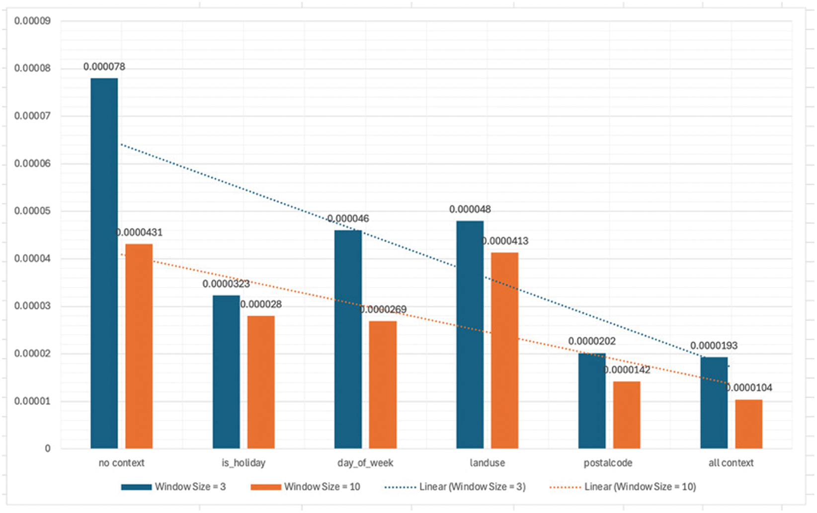 Fig. 9. Performance of STC-LSTM under different contextual configurations.
C.DISCUSSION
This section presents an in-depth discussion of the experimental findings, interpreting the observed performance differences among contextual configurations and relating them to the underlying characteristics of spatio-temporal mobility patterns. We analyze how integrating semantic context influences prediction accuracy, examine the implications of window size and model design choices, and situate the results within the broader literature on next-location prediction.
Adding contextual information is essential for capturing the regularity and underlying structure of user movement behavior, as mobility patterns are often influenced by spatial–temporal coordinates, as well as semantic and environmental factors. The percentage improvement analysis further highlights the advantage of incorporating contextual information into spatio-temporal mobility prediction. As shown in Fig. 10 (a), all context-aware configurations achieve substantial reductions in prediction error compared to the baseline model that relies solely on trajectory data, with improvements ranging from approximately 38% to over 75%. This result indicates that spatial–temporal coordinates alone are insufficient to fully characterize user mobility behavior. In particular, the strong performance gains observed when integrating postal code and land-use information demonstrate the importance of fine-grained spatial semantics in capturing localized movement patterns. Moreover, the consistently superior performance of the all-context configuration confirms that temporal and spatial contextual features provide complementary information, enabling the model to learn richer and more discriminative representations of mobility. Compared with previous studies that primarily focus on raw trajectory sequences, the proposed STC-LSTM framework offers a more comprehensive modeling approach by explicitly incorporating semantic context, leading to significantly improved prediction accuracy and more robust next-location forecasting.
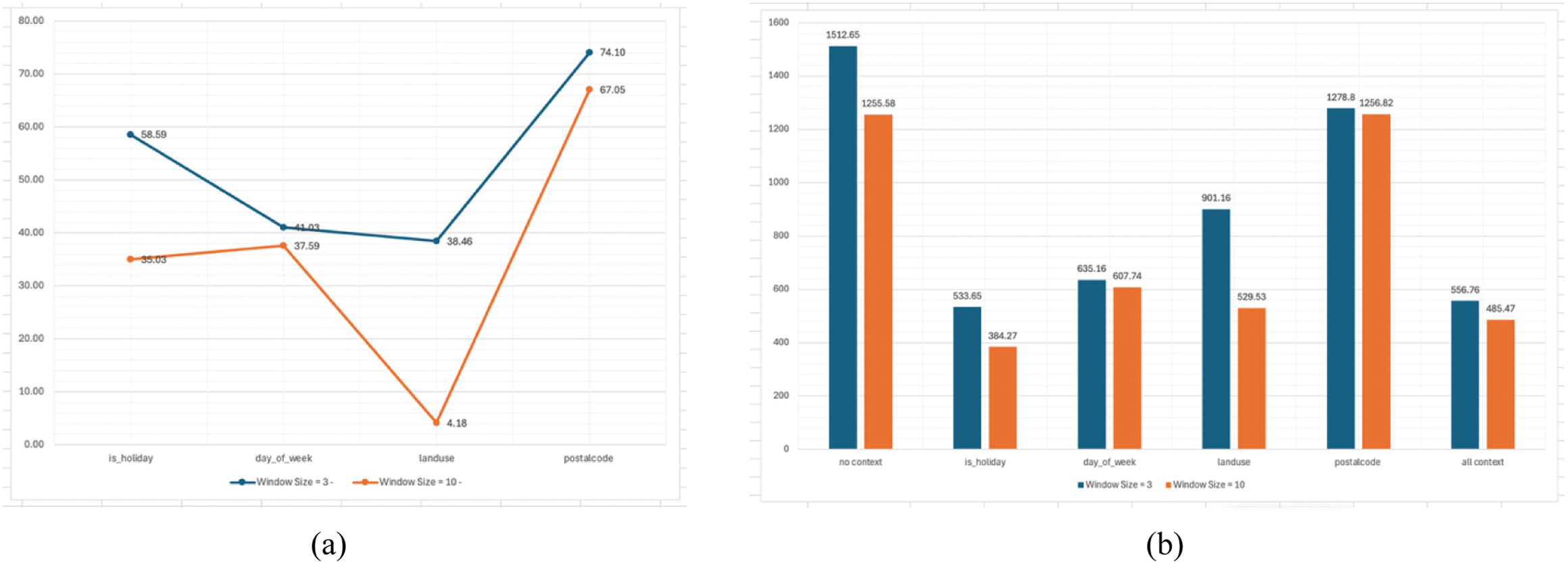 Fig. 10. Contribution of contextual features to (a) prediction performance and (b) spatial accuracy.
Furthermore, Fig. 10(b) shows the average spatial error, measured as the difference in distance (in meters) between the predicted and actual next locations, across different contextual configurations and window sizes. The baseline model without contextual information exhibits the largest prediction error, with average distances exceeding 1.5 km for a window size of 3 and 1.25 km for a window size of 10. This result confirms that relying solely on raw trajectory coordinates limits the model’s ability to accurately capture user movement behavior.
Incorporating contextual information leads to substantial reductions in spatial error across most configurations. Among individual contexts, the inclusion of holiday information (is_holiday) yields the most significant improvement, reducing the average error to 533.65 m (window size 3) and 384.27 m (window size 10). This suggests that holiday-related temporal context significantly influences mobility patterns and substantially improves next-location prediction accuracy. The day-of-week context also improves performance, reflecting the presence of regular weekly mobility routines. The land-use context yields moderate improvements, particularly for the larger window size, indicating that the functional characteristics of locations become more informative when longer historical trajectories are considered. In contrast, the postal code context alone yields relatively limited gains and, in some cases, performance comparable to the baseline. This indicates that while postal codes offer fine-grained spatial semantics, their limited gains suggest that relying solely on them may not sufficiently improve practical mobility predictions without additional contextual cues. The all-context configuration consistently achieves low spatial error across both window sizes, demonstrating that integrating multiple contextual cues provides complementary benefits. By jointly modeling temporal regularities and spatial semantics, the STC-LSTM framework significantly improves the practical accuracy of next-location prediction, reducing average spatial error by more than half compared to the baseline. These results further support the conclusion that context-aware modeling is essential for reliable and realistic spatio-temporal mobility prediction.
An illustrative example of next-location prediction is presented in Fig. 11. The STC-LSTM model is trained on the complete trajectory dataset and subsequently evaluated on an unseen individual trajectory. At each time step, the model predicts the subsequent spatial position based on historical movement and contextual information. In the figure, the ground-truth next locations are indicated by red markers, while the model-generated predicted locations are shown in blue. The visual comparison demonstrates that the predicted trajectory closely follows the actual movement pattern, highlighting the model’s ability to capture both spatial continuity and directional consistency in real-world mobility scenarios.
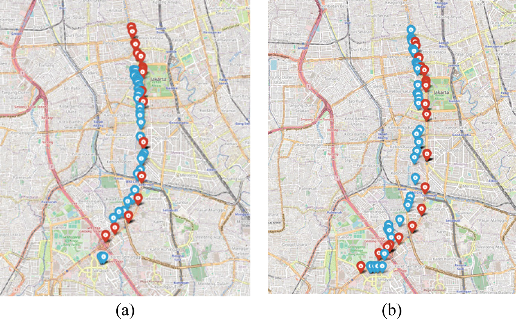 Fig. 11. Next-location prediction results using the all-context STC-LSTM model for trajectory ID 23648 with window sizes of (a) 3 and (b) 10.
Although incorporating contextual information significantly reduces spatial prediction error, the remaining average distance error still exceeds 300 meters in the best-performing configurations, indicating substantial room for improvement. Future work may investigate more advanced modeling strategies, such as diffusion-based generative models to capture the uncertainty and multi-modal nature of human mobility, as well as agent-based modeling frameworks that explicitly simulate individual decision-making and movement dynamics. Combining context-aware deep learning with diffusion or agent-based approaches, potentially constrained by road network topology, and incorporating richer contextual signals, including real-time traffic conditions, user activity semantics, and point-of-interest dynamics, may enable finer-grained spatial predictions and further reduce residual location error.
V.CONCLUSION
This study investigated next-location prediction in spatio-temporal trajectory data by explicitly integrating contextual information into a deep learning framework based on LSTM. Using a large-scale real-world dataset comprising approximately 56,000 trajectories or 5.6 million GPS points, we proposed the STC-LSTM model, which incorporated temporal and spatial semantic contexts, including day of the week, holiday indicators, land use, and postal codes. The experimental pipeline included rigorous preprocessing steps such as trajectory cleaning and map-matching, followed by contextual annotation, normalization, and model training with stacked LSTM and dropout layers. Extensive evaluations demonstrated that context-aware modeling substantially improves prediction accuracy compared to trajectory-only approaches (without context). The all-context configuration consistently outperformed individual context and baseline models, achieving the lowest MSE of 1.04 × 10⁻⁵ with a window size of 10, while the no-context baseline recorded the highest error of 7.80 × 10⁻⁵. Specifically, incorporating contextual information improved prediction accuracy by approximately 38% to over 75%.
Beyond numerical error reduction, distance-based evaluation further confirmed the benefit of contextual enrichment in improving spatial prediction quality. Although integrating context information significantly reduced prediction error, residual spatial inaccuracies remain, indicating opportunities for further refinement. Future research will focus on enhancing spatial semantic assignment by leveraging full-polygon and multipolygon geometries from OpenStreetMap (OSM) rather than centroid-based representations, enabling more precise modeling of land-use and postal code boundaries. Additionally, extending the framework to support multi-step prediction and incorporating advanced modeling strategies, such as diffusion-based generative models or agent-based mobility representations, may further improve predictive realism and robustness. Future studies will also investigate the generalizability of the proposed STC-LSTM framework through cross-dataset evaluation on mobility datasets with varying characteristics, including sparse and dense trajectories, different sampling frequencies, and diverse contextual attributes. Such evaluations will provide deeper insights into the robustness of context-aware mobility modeling across heterogeneous mobility environments. Overall, this study highlighted the critical role of contextual information in spatio-temporal modeling and provided a strong foundation for developing more accurate and reliable next-location prediction systems.