JAIT

I.INTRODUCTION

Accurate mortality prediction is the primary determinant in actuarial frameworks, providing essential information for actuarial pricing, including reserve valuation for life insurance and pension solvency assessment. Inaccurate modeling of mortality projection may impose a profound financial risk. For instance, underestimating mortality rates can result in underpriced premiums and underfunded liabilities, while overestimating the rate of mortality decline may lead to excessive pension payouts due to longevity risk. Robust mortality models are therefore essential for capturing survival dynamics in aging populations and supporting the long-term sustainability of life insurance and pension systems.

Malaysia is projected to transition into an aged nation by 2030, a demographic shift accelerated by a continuous decline in mortality and a decline in total fertility rates from 3.3 to 1.9 children per woman over the last four decades [1]. According to the Department of Statistics, Malaysia [2], life expectancy at birth has increased substantially from 71.2 years in 1990 to 75.2 years in 2024. While the increasing life expectancy trend reflects significant improvements in health and longevity, this demographic transition places greater pressure on pension systems and increases the need for accurate mortality forecasting models.

Mortality forecasting models have evolved from deterministic to stochastic methods that are capable of addressing data complexities. Prior to the 1990s, mortality modeling was dominated by conservative parametric models, such as the Gompertz [3] and Makeham [4], that relied on periodic life tables to extrapolate trends. While the Heligman–Pollard (HP) model [5] introduced greater flexibility through multi-component age-group representation, its application for long-term projection is frequently compromised by high parameter dimensionality. This complexity often leads to overfitting and increased residuals, limiting its efficacy in large-scale demographic data.

A major turning point occurred in 1992 with the introduction of the Lee–Carter (LC) bilinear regression model [6]. The LC model provided a robust and widely adopted framework for predicting mortality rates. There are two factors simultaneously incorporated in the model, namely the age component $(b_{x})$ and the time component $(k_{t})$ . While the first captures the age-specific sensitivity of mortality rates to temporal changes, the second represents the general level of mortality over time. This bi-factor LC model [6] can be formulated as a nonlinear specification in which age and time are treated as factors with a homoscedastic and normally distributed error term [7]. The model decomposes the logarithm of the central mortality rate into three primary elements, the average age-specific mortality rate $(a_{x})$ in addition to $k_{t}$ and $b_{x}$ . This approach enables the model to distinguish between age-related variation in mortality and time-dependent changes, making it significantly more reliable than conservative parametric approaches.

Although the LC model [6] has been widely used in mortality forecasting, it has several limitations. The model assumes that mortality is invariant across ages, which limits its ability to capture heterogeneous age-specific changes over time, particularly among children and the oldest-old. In addition, the LC model does not account for cohort effects, thereby overlooking generational differences in mortality patterns arising from varying lifestyles, environmental exposures, or medical influences. The stochastic structure of the traditional model, which typically models the time component as a random walk with drift, is viewed as insufficient to capture complex uncertainties and as potentially underestimating longevity risk.

To address these limitations, various extensions have been proposed. For example, the Renshaw–Haberman model [8] incorporates cohort effects, thereby enhancing its capacity to capture intergenerational variation. The Cairns, Blake, and Dowd (CBD) model [9] was developed and tailored for older age groups and introduces multiple period factors, making it particularly suitable for pension and annuity applications. More flexible approaches, such as functional data methods [10], have also been developed, offering improved accuracy in capturing complex mortality patterns and delivering more robust long-term forecasts. In addition, coherent mortality models [11] have been developed to jointly model multiple populations and avoid divergence in long-term forecasts, with recent studies confirming their improved performance [12–14].

Despite the growing number of extended models proposed in the literature, the choice of an appropriate fitting period is often overlooked. This remains an important gap, as the selection of the fitting period plays a crucial role in determining the accuracy and reliability of mortality forecasts. Most existing studies assumed fixed fitting periods without testing whether the chosen period yields optimal accuracy. An inadequately chosen fitting period may produce biased model estimates, resulting in significant out-of-sample prediction errors. According to Ibrahim et al. [15], the time $(k_{t})$ and the age $(b_{x})$ components of the LC model are sensitive to the chosen fitting period, as different periods capture different structural fluctuations in mortality trends. Therefore, inappropriate selection of the fitting period may lead to biased parameter estimates and inaccurate projections.

Based on this gap, this research aims to develop a hybrid LC mortality forecasting framework that integrates optimized fitting period selection with stochastic time-series models (auto-regressive integrated moving average (ARIMA)) and machine learning methods, specifically artificial neural networks (ANNs) and random forests (RFs), for forecasting the time component $k_{t}$ of the model. The predictive performance of the proposed models is systematically evaluated using out-of-sample forecasting error metrics. The best-performing model is then used to generate mortality rate projections by age and gender for the Malaysian population.

The key contributions of this research are as follows:

•It develops a hybrid LC mortality forecasting framework that integrates optimized fitting period selection with stochastic time-series (ARIMA) and machine learning methods (ANN and RF) to improve the estimation of the time component of the model.
•It provides a systematic comparison of LC-ARIMA, LC-ANN, and LC-RF models, offering practical evidence on how ARIMA and machine learning approaches perform under different fitting period configurations.
•It also highlights the importance of selecting an appropriate fitting period, showing how this can improve the accuracy and stability of mortality parameter estimations.
•Since the framework is applied to Malaysian mortality data from 1980 to 2024, this contributes to new empirical insights from a developing country with a rapid aging population growth.

The remainder of this article is structured as follows. Section II provides a critical review of the relevant literature and foundational mortality frameworks, specifically on the selection of the fitting period. Section III describes the proposed methodology and algorithmic design. Section IV presents a comprehensive analysis of the empirical findings and performance metrics. Finally, Section V offers concluding remarks and future research directions, followed by the acknowledgments and references.

II.RELATED WORKS

The traditional LC model established the basis for stochastic mortality predictions. However, its assumptions, such as a single universal mortality trend across all ages and the exclusion of cohort effects, restrict its efficiency, especially in populations undergoing rapid changes [16,17]. As a result, several modifications and extensions have been introduced by many researchers to capture a better understanding of the complex dynamics of mortality pattern forecasting.

Concerns about the selection of an appropriate fitting period started as early as research by [18], which provided a detailed assessment of the traditional LC model’s predictive accuracy. In their study, the model was tested by using different historical subsamples. Forecasts started with data from 1900 to 1920 and then gradually extended year by year until 1900–1997, which produced a forecast for 1998. This approach generated 78 one-year-ahead forecasts, 77 two-year-ahead forecasts, and longer-horizon forecasts extending up to 78 years. For each subsample, the parameters $a_{x}$ and $b_{x}$ were re-estimated over the fitting period, and the time-varying component $k_{t}$ was modeled as a stochastic drift process using ARIMA (0,1,0), maintaining structural consistency with the original framework. The findings indicated that longer fitting periods, combined with shorter forecast horizons, resulted in lower forecast errors.

Moreover, Tuljapurkar et al. [19] suggested a simple and satisfactory solution to fitting period problems by using the base of the forecast on data from 1950, instead of 1900, as was originally done by Lee and Miller [18]. This adjustment is assumed to be invariant $b_{x}$ over the first half century, irrespective of the total observational period. Booth et al. [20] identified the optimized fitting period based on the period displaying an approximately linear decreasing pattern in the time-varying component $k_{t}$ . The methodology employs a fixed-horizon ending point, whereas the initial year $(S)$ was optimized to ensure the fitting period produces a near-linear trajectory pattern. The model determined the fitting period through a judgment-based assessment of the observed patterns of both $b_{x}$ and $k_{t}$ , with the latter constrained to exhibit a linear decreasing pattern, and subsequently modeled using the ARIMA approach.

Ibrahim et al. [15] examined Malaysian mortality dynamics through the traditional LC framework and explored two alternative fitting periods, including 1970–1993 and 1970–2000. To estimate in-sample goodness-of-fit, the researchers employed the Akaike information criterion (AIC) and Bayesian information criterion (BIC), while out-of-sample predictive stability was quantified via mean absolute percentage error (MAPE) and root mean square error (RMSE). Their findings revealed that the constrained fitting period achieved a superior fit and enhanced forecast accuracy for females, suggesting that extended temporal horizons may introduce stochastic noise rather than improve forecast accuracy.

In the traditional LC framework, the estimated $k_{t}$ is typically extrapolated using linear time-series models, such as a random walk with drift. However, these models impose strong assumptions of linearity and stationarity, which may limit their ability to capture nonlinear mortality dynamics, structural changes, and heterogeneous age-specific changes.

To address these limitations, recent studies have incorporated machine learning methods into the LC framework for forecasting $k_{t}$ . Hong et al. [21] demonstrated that ANNs and RF models are more effective in capturing nonlinear patterns in mortality time series. Unlike ARIMA-based approaches, these models do not rely on strict assumptions such as linearity or stationarity. This allows them to better handle complex relationships and interactions within the data, resulting in greater flexibility and improved predictive accuracy. Furthermore, integrating ANN and RF into the LC framework enhances forecasting performance by improving the estimation of the time component $k_{t}$ while maintaining robustness without extensive parametric specification. Hong et al. [21] also explored both the effects of time-varying indices and age-component invariance within the LC model to select the optimum fitting period. Their research applied two machine learning algorithms, namely ANN and RF.

While studies have explored various methods to identify optimal fitting periods for mortality forecasting, relatively few have examined both ARIMA stochastic processes and machine learning models within the LC framework, and none have focused on Malaysian mortality data. Although several studies have applied machine learning models to Malaysian datasets [22–24], the integration of machine-learning–based prediction within the LC framework remains limited, and the selection of an optimized fitting period has been ignored. In particular, there is a gap in the direct comparative analysis of the LC-ARIMA, LC-ANN, and LC-RF models under optimized fitting periods.

Accordingly, this research develops a hybrid LC mortality forecasting framework that integrates optimized fitting period selection with alternative approaches for forecasting the time component $k_{t}$ , including stochastic time-series models (ARIMA) and machine learning methods, namely ANNs and RFs. Within this framework, the predictive performance of LC-ARIMA, LC-ANN, and LC-RF models is systematically evaluated and compared using out-of-sample error metrics. Based on the model demonstrating the highest predictive accuracy, future mortality rates of the Malaysian population are forecasted, from which life expectancy estimates and mortality improvements are derived.

III.METHODOLOGY

A.MORTALITY DATA PREPROCESSING

Yearly mortality data by age (0–75) and gender for the period 1980 to 2024 were obtained from the National Statistics Department of Malaysia. Disaggregation data by male and female populations is performed to allow age- and gender-specific mortality analyses. Rainbow plots were generated in R using the demography package by Hyndman et al. [25] to visualize temporal and age-specific mortality patterns. These visualizations provided an overview of the evolution of mortality across ages and calendar years.

The raw data were reported in five-year age intervals. These data were smoothed to obtain single-year age data using the smooth.demogdata function in R. This procedure reduced random variation and measurement noise while preserving the underlying mortality structure. This preprocessing step improved the stability of the model’s parameter estimation and reduced outliers during subsequent forecasting. In addition, life expectancy by gender was computed to support the interpretation of mortality trends and to provide an aggregate summary measure consistent with the age-specific mortality patterns observed in the data.

To determine the optimal fitting period, we conducted a comparative performance analysis across various observational periods. Out-of-sample accuracy was assessed through mean absolute error (MAE) and RMSE. The optimal fitting period was chosen based on the period that yielded the minimum forecast errors.

B.MORTALITY FORECASTING MODEL

1).THE BASELINE LC MODEL

The traditional LC model was employed as the baseline statistical approach. The model expresses the logarithmic central mortality rate as a bilinear combination of age and time factors, as shown in Equation (1):

\log (m_{x, t}) = a_{x} + b_{x} k_{t} + ɛ_{x, t}

(1)

In this formulation, $m_{x, t}$ denotes the observed mortality rate for a specific age $x$ during year $t$ for either male or female. The term $a_{x}$ represents the respective average log mortality over the observed years and $b_{x}$ captures the sensitivity of specific age mortality to fluctuations in time index, $k_{t}$ . This time index captures the overall stochastic progression of mortality. The residual variance is accounted for by the error term $ɛ_{x, t}$ .

To determine the model’s structural parameters, a singular value decomposition (SVD) was performed on the matrix of mean-adjusted log-mortality rates. This estimation process was performed under the standard constraints of $\sum_{x} b_{x} = 1$ and $\sum_{t} k_{t} = 0$ .

Furthermore, $k_{t}$ serves as the stochastic time component within the framework, which requires an econometric forecasting approach. In this study, the temporal trajectory of $k_{t}$ was modeled through an ARIMA model. To achieve statistical stationarity, appropriate differencing orders were applied, while the optimal lag structure was identified by minimizing the AIC and BIC. The general mathematical specification for the ARIMA process is provided in Equation (2):

{\hat{k}}_{t} = c + {\emptyset︀}_{1} k_{t - 1} + \dots + {\emptyset︀}_{p} k_{t - p} + ɛ_{t} + θ_{1} ɛ_{t - 1} + \dots + θ_{q} ɛ_{t - q}

(2)

where

k_{t - p}

is the observed time component value for the previous year

t - p

, or lagged values, while

ɛ_{t}

denotes a white noise error term, and

\emptyset︀

and

θ

are the model’s estimating parameters.

The forecasted mortality time component ${\hat{k}}_{t}$ was then integrated into the LC model together with the estimated $b_{x}$ and $a_{x}$ to obtain projected values of mortality rates according to age and gender, as shown in Equation (3):

{\hat{m}}_{x, t} = e x p (a_{x} + b_{x} {\hat{k}}_{t})

(3)

2).ARTIFICIAL NEURAL NETWORK (ANN)

Instead of forecasting the LC time component, $k_{t, i}$ using time-series ARIMA model, this study employed the ANN to capture potential nonlinear dynamics in mortality trends. Lagged values of the estimated $k_{t, i}$ served as inputs to the ANN, and the forecast values were subsequently incorporated into the LC framework to obtain age-specific mortality projections.

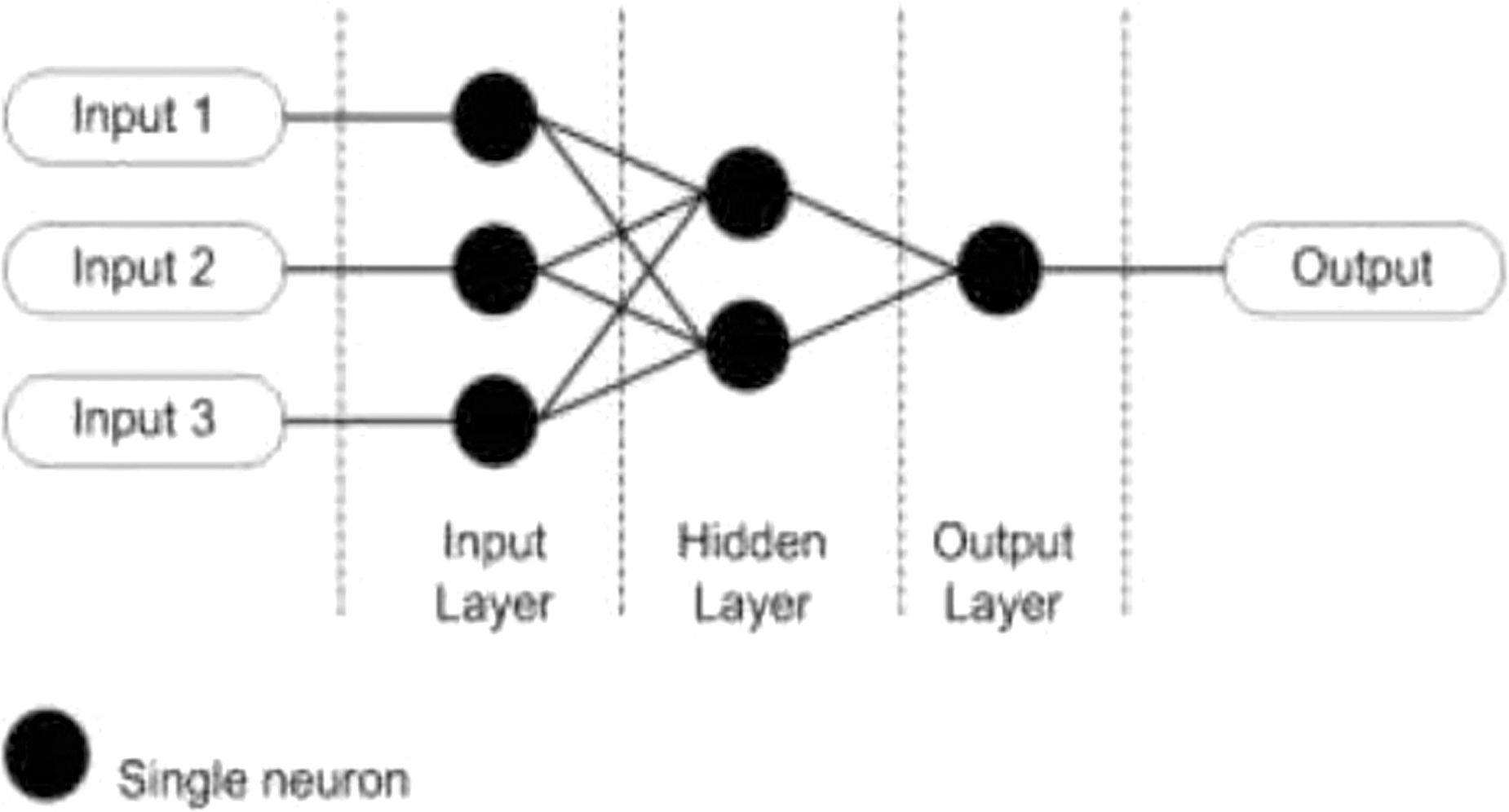
Following Hong et al. [21], a feed-forward multilayer perceptron (MLP) architecture was employed. The system consisted of an input layer containing p neurons corresponding to lagged values of $k_{t, i}$ , a single hidden layer with nonlinear activation functions, rectified linear unit (ReLU), and a single output neuron, which produced the predicted value $k_{t}$ . This ANN model was trained to produce forecast future $k_{t}$ values. The network structure was tuned by adjusting the number of hidden neurons and training epochs. Input data were normalized before training and denormalized after prediction. The model’s architectural components are summarized as follows:

•An input layer at time t: lagged values of $k_{t, i}$ $(k_{t, i - 1}, k_{t, i - 2} \dots .. k_{t, i - p})$ , where $p$ denotes the length of the fitting data in terms of number of years;
•A single hidden layer with ReLU activation;
•An output layer to produce predictions of future $k_{t, i}$ .

As illustrated in Fig. 1, the feed-forward ANN architecture indicates that data move in one direction linearly across layered neurons. The implementation of the ANN model involved the following procedural stages:

1.The extracted observed mortality index $k_{t}$ derived from the LC model was stratified into training and validation datasets.
2.To improve learning accuracy, $k_{t}$ was normalized using the following formula:
${k_{t, i}}^{norm} = \frac{k_{t, i} - μ}{σ}$ (3)
where $μ$ denotes the mean of the in-sample data which used as the training datasets and $σ$ denotes the standard deviation of the data.
3.The training data were used as the inputs to the ANN. Determination of the optimized hidden neuron layer was achieved through an iterative trial and validation framework. We compare various architectural iterations against standard performance metrics, selecting the one that yielded the minimum forecast errors.
4.The model generated forecasts of normalized $k_{t}$ values, which were then demoralized. The projected ${\hat{k}}_{t}$ indices were subsequently integrated with the previously estimated parameters $b_{x}$ and $a_{x}$ from the LC, to generate mortality projections.

Fig. 1. A feed-forward ANN structure (Hong et al. [20]).

3).RANDOM FOREST (RF)

Consistent with Hong et al. [21], the RF method employed an ensemble of decision trees to predict future values of $k_{t}$ . Hyperparameter optimization focused on the total tree counts and variables per split were performed using out-of-bag (OOB) errors. The RF modeling procedure was conducted in these steps:

1.Similar to the ANN, the extracted observed mortality index $k_{t}$ from the LC model was stratified into training and validation datasets.
2.Key hyperparameters, such as trees and splitting variable counts, were tuned based on the OOB error plot. The best combination was selected for final training.
3.The trained RF model was used to forecast the re-estimated $k_{t, i}$ values for both genders.

C.EVALUATION OF THE OPTIMIZED FITTING PERIOD

To identify the optimal historical fitting period, the data were divided into training and validation subsets. The mortality dataset covered the period from 1980 to 2024. The initial training set comprised observations from 1980 to 2002, while the remaining data from 2003 to 2024 were reserved for testing. This split resulted in an approximately 50:50 ratio between the training and testing samples. The training and validation datasets are illustrated in Fig. 2.

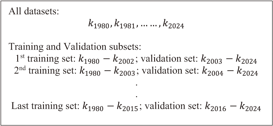Fig. 2. Illustration of the full dataset, divided into training (fitting) and testing (out-of-sample) sets.

The process was repeated iteratively by extending the training window forward by one year at each step. This evaluation continued until the final training period, which ranged from 1980 to 2015, with the corresponding testing period covering from 2016 to 2024, resulting in an 80:20 split. Each model was fitted using the training set and tested on the out-of-sample data. The accuracy of predicted values was assessed through MAE and RMSE, as defined in Equations (4) and (5) respectively, as below:

M A E = \frac{1}{N} \sum_{i = 1}^{N} | m_{x, t} - {\hat{m}}_{x, t} |

(4)

R M S E = \sqrt{\frac{1}{N} \sum_{i = 1}^{N} m_{x, t} - {\hat{m}}_{x, t}^{2}}

(5)

The models were compared across gender and age groups based on these error values. The optimal fitting period was selected as the one that yielded the lowest forecast error, measured by both MAE and RMSE.

D.MORTALITY IMPROVEMENT AND LIFE EXPECTANCY

The best-performing model was then applied to forecast future mortality rates from 2025 to 2038. Based on these forecasts, life expectancy at birth and mortality improvement rates were calculated. Annual (year-over-year) mortality improvement at age $x$ , denoted as $M I_{x, t}$ , and the geometric (multi-year average) mortality improvement, denoted as $M I_{x, t, t + n}$ , are defined in Equations 6 and 7, respectively, as follows:

M I_{x, t} = (1 - \frac{m_{x, t + 1}}{m_{x, t}}) \times 100

(6)

M I_{x, t, t + n} = (1 - {(\frac{m_{x, t + n}}{m_{x, t}})}^{\frac{1}{n}}) \times 100

(7)

Meanwhile, the forecasted life expectancy was measured using the Actuarial Life Table approach. The projected mortality rates were transformed into $q_{x, i}$ , which denotes the probability that an individual either male or female dies between age $x$ and $x + n$ . A standard radix of 100,000 was used to initialize the synthetic cohort at birth, denoted by $l_{o}$ . Next, $l_{x}$ , which denotes the survivor counts derived at the initial age interval, and, $d_{x}$ , which denotes the number of deaths derived within the interval, were estimated using Equations (8) and (9):

l_{x + 1} = l_{x} \cdot (1 - q_{x})

(8)

d_{x} = l_{x} - l_{x + 1}

(9)

The person-years survived within each age interval, denoted by $L_{x}$ , was estimated under the uniform distribution assumption within the interval. The probabilities of survival and death are estimated only over a single-year period. In order to obtain the overall survival probabilities, the survival probabilities for each individual year were multiplied by the probability of a person surviving from age $x$ to $x + t$ :

L_{x} = l_{x + 1} + \frac{d_{x}}{2}

(10)

The person-years survived after age $x$ , denoted as $T_{x}$ , was computed by cumulatively summing $L_{x}$ from that age onward:

T_{x} = \sum_{y = x}^{\infty} L_{y}

(11)

Finally, life expectancy, denoted as $e_{x}$ , was calculated using the following formula:

e_{x} = \frac{T_{x}}{l_{x}}

(12)

IV.RESULTS AND DISCUSSION

This study explores the choice of an appropriate fitting period for mortality forecasting using Malaysian mortality data from 1980 to 2024. Four forecasting approaches were evaluated: the traditional LC model, the LC ARIMA model, and two machine learning approaches, namely LC-ANN and LC-RF. The analysis focused on identifying optimized fitting periods that minimize forecast errors and yield more reliable mortality predictions.

The analysis commences with an assessment of historical mortality patterns and life expectancy trends among the Malaysian population by age and gender. Subsequently, various fitting-period configurations are evaluated to determine the optimal fitting periods that minimize forecast errors across the selected model variants. The model with the highest predictive performance is then used to generate future mortality forecasts. Finally, projected mortality improvements are examined to provide insights into future longevity trends.

A.TRENDS IN MORTALITY AND LIFE EXPECTANCY

Figure 3 displays rainbow plots of smoothed historical mortality rates for both genders on a logarithmic scale from 1980 to 2024. The plot provides a clear visualization of how mortality has evolved over time. The age pattern of mortality is a fundamental component of mortality modeling, as mortality risks vary substantially with age due to differences in biological processes and causes of death. Ignoring age variation in mortality forecasting may therefore compromise the accuracy of projected mortality rates.

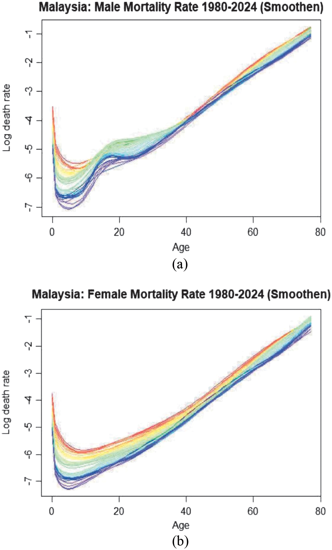Fig. 3. Malaysian mortality rates by age and gender, including males (a) and females (b), from 1980 to 2024.

As illustrated in Fig. 3, mortality rates increase nearly exponentially with age, with infants and older adults being the most vulnerable groups. The oldest exhibit substantially higher mortality rates due to high risk diagnosed with chronic diseases and the cumulative effects of multiple identifiable age-related risk factors associated with senescence [26]. These age-mortality patterns remain consistent for both Malaysian males and females across the study period. Mortality trends by year show a clear downward shift in the mortality curves from initial years (red shades) to more recent years (violet shades), indicating substantial improvements in mortality.

Notably, significant declines in mortality rates are observed at younger and older ages throughout the study period. A comparison between genders shows that mortality declines among females appear more gradual and stable over time, whereas male mortality trends show some fluctuations, especially during the presence of an accident hump among young male groups.

In terms of mortality improvement, a substantial reduction is observed among infants and young children, as indicated by the wide gap between the red and purple lines, which denote early and recent mortality curves, respectively. This suggests significant gains in survival for this age group. In contrast, the gap between curves is narrower for individuals aged 40 to 60 years, particularly among males, indicating that mortality improvements in this middle-aged group have been relatively limited.

Life expectancy at birth was computed using the mortality rates and the life table formulation described in Equations (10–12). Figure 4 shows a steady rise in Malaysian life expectancy over more than four decades, with women’s life expectancy consistently higher than that of men. In 2024, Malaysian life expectancy reached 83 and 74 years for women and men, respectively. Malaysia experienced a temporary decline in life expectancy in 2020–2021, largely due to excess mortality during the COVID-19 pandemic. This included both direct deaths from COVID-19 and indirect effects such as disruptions to healthcare services. In particular, 2021 saw a significant surge in excess mortality during the peak waves of the pandemic, with deaths exceeding expected levels and contributing to the deterioration in overall mortality outcomes during this period. [27]. In terms of the overall percentage, life expectancy increased by approximately 3% for every 10 years over the recorded study period.

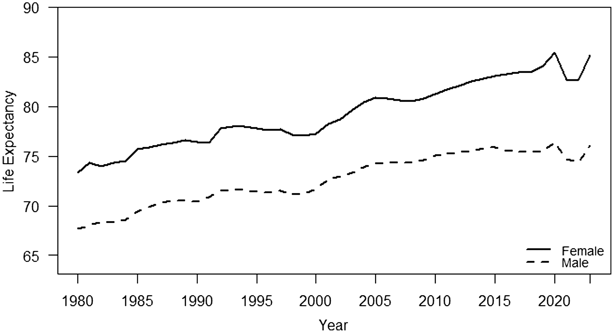Fig. 4. Malaysian life expectancy for males and females from 1980 to 2024.

B.OPTIMAL FITTING PERIODS FOR MORTALITY FORECASTING MODELS

All forecasting models were evaluated using out-of-sample forecasting error metrics, including MAE and RMSE. Results indicate that each forecasting model exhibits a different optimal fitting period for achieving the most accurate mortality forecasts.

Table I presents the LC-ARIMA model’s predictive performance across varying fitting or training periods. The results indicate that the model’s accuracy is highly dependent on the selection of the fitting period. The optimized fitting period for the male population was achieved in 1980–2002, whereas the female population reached its minimum errors in 1980–2004. Generally, extending the training period, particularly toward 2015, led to a progressive increase in forecast errors.

Table I. Forecast performance accuracy of the LC-ARIMA model by genders

Training period	Male		Female
Training period	MAE	RMSE	MAE	RMSE
1980–2002	0.002244	0.004356	0.003366	0.007094
1980–2003	0.002245	0.004567	0.002385	0.005036
1980–2004	0.002811	0.005795	0.002026	0.004177
1980–2005	0.003352	0.006797	0.002046	0.004276
1980–2006	0.003129	0.006427	0.002089	0.004321
1980–2007	0.002399	0.005161	0.002272	0.004742
1980–2008	0.002306	0.004896	0.002442	0.005168
1980–2009	0.002510	0.005454	0.002373	0.005029
1980–2010	0.003252	0.006720	0.002136	0.004443
1980–2011	0.003295	0.006779	0.002091	0.004277
1980–2012	0.003320	0.006798	0.002132	0.004290
1980–2013	0.003368	0.006862	0.002268	0.004414
1980–2014	0.003698	0.007293	0.002446	0.004632
1980–2015	0.003239	0.006497	0.002656	0.004878

Tables II and III show the predictive performance of the machine learning-based models, specifically the LC-ANN and LC-RF models. In contrast to the ARIMA-based framework, these models demonstrate a significant capacity to utilize more extensive historical datasets to improve prediction accuracy. For instance, the LC-ANN model achieves its optimal predictive performance with a medium- to long-term training period. For the male population, the model achieved its lowest error during 1980–2010, while the female population reached its lowest error during 1980–2013. The initial high errors in the 1980–2002 period suggest that the neural network requires longer fitting data to effectively learn the nonlinear dynamics of mortality transitions. However, the observed increase in errors after 2013 toward the 2015 horizon indicates a potential threshold beyond which incorporating more recent data introduces greater volatility in mortality patterns.

Table II. Forecast performance accuracy of the LC-ANN model by genders

Training period	Male		Female
Training period	MAE	RMSE	MAE	RMSE
1980–2002	0.006515	0.012319	0.008877	0.017647
1980–2003	0.003507	0.006752	0.004675	0.008326
1980–2004	0.004630	0.008522	0.008617	0.016711
1980–2005	0.005320	0.009834	0.004285	0.008250
1980–2006	0.002477	0.004604	0.003462	0.008274
1980–2007	0.002348	0.004530	0.004319	0.009819
1980–2008	0.002785	0.005418	0.004616	0.010341
1980–2009	0.002491	0.004843	0.004547	0.010252
1980–2010	0.001986	0.003908	0.003822	0.009063
1980–2011	0.002132	0.004244	0.002700	0.006804
1980–2012	0.002215	0.004349	0.002169	0.005376
1980–2013	0.002330	0.004525	0.002114	0.004778
1980–2014	0.002628	0.005039	0.002300	0.005237
1980–2015	0.002662	0.004944	0.002494	0.005495

Table III. Forecast performance accuracy of the LC-RF model by genders

Training period	Male		Female
Training period	MAE	RMSE	MAE	RMSE
1980–2002	0.011341	0.020843	0.010983	0.020838
1980–2003	0.011615	0.021226	0.011255	0.021284
1980–2004	0.011566	0.021318	0.011340	0.021555
1980–2005	0.011618	0.021446	0.011465	0.021988
1980–2006	0.011613	0.021502	0.011485	0.022067
1980–2007	0.011524	0.021638	0.011381	0.022214
1980–2008	0.011290	0.021219	0.011393	0.022251
1980–2009	0.010767	0.020677	0.011174	0.022324
1980–2010	0.010513	0.020313	0.011288	0.022355
1980–2011	0.010221	0.019830	0.010834	0.021650
1980–2012	0.009450	0.018472	0.010102	0.020973
1980–2013	0.007028	0.015189	0.008623	0.018603
1980–2014	0.005683	0.012363	0.007540	0.016771
1980–2015	0.005063	0.011489	0.006573	0.015689

Table III illustrates the performance of the LC-RF model, which exhibits a distinct “learning curve” characterized by a continuous reduction in error as the training period extends. Unlike all other evaluated models, the LC-RF model produced the most accurate forecasts when the full fitting period from 1980 to 2015 was used for both genders. This indicates the stability of the RF model, particularly when using 500 decision trees. The model effectively mitigates variance and avoids overfitting, even as the dataset becomes more complex. This rigorous analysis, across multiple training and fitting periods, provides a robust framework for accurate mortality prediction.

Table IV summarizes the predictive performance and optimal fitting periods for the evaluated mortality models. The LC-ANN model outperforms other models, achieving the lowest average MAE of 0.00205 and particularly high precision for the male population. While the LC-ARIMA model also demonstrated strong competitive accuracy (average MAE: 0.00214), it required significantly more constrained temporal windows, with fitting periods ending in 2002 and 2004, to achieve its optimal performance. In contrast, the LC-ANN and LC-RF models utilized more recent data (2010 to 2015), suggesting that the machine learning approaches are more adept at internalizing recent structural shifts in mortality trends. Although the LC-RF model exhibited higher error rates than the LC-ANN, it maintained stable performance over extended fitting periods.

Table IV. Summary of optimal fitting periods for the selected mortality forecasting models among males (M) and females (F)

Model	Gender	Optimal fitting period	Min MAE	Average MAE
LC	M	1980–2012	0.00430	0.00503
LC	F	1980–2012	0.00576	0.00503
LC-ARIMA (0,1,1)	M	1980–2002	0.00224	0.00214
LC-ARIMA (0,1,0)	F	1980–2004	0.00203	0.00214
LC-ANN (one neuron with one hidden layer	M	1980–2010	0.00199	0.00205
LC-ANN (one neuron with one hidden layer	F	1980–2013	0.00211	0.00205
LC-RF (500 trees)	M	1980–2015	0.00506	0.01359
LC-RF (500 trees)	F	1980–2015	0.00657	0.01359

Collectively, these findings provide a robust, data-driven justification for adopting hybrid LC mortality prediction frameworks. Our study proved that the incorporation of an optimized fitting period reduces forecast error by ensuring that model estimation is based on the most suitable fitting window, thereby increasing prediction accuracy of mortality rates. While stochastic LC-ARIMA remains effective for capturing short-term trends, LC-ANN demonstrates superior mortality predictions. This finding is consistent with [21] who compared LC, LC-ANN, and LC-RF models and found that ANNs improved predictive accuracy by better capturing nonlinear mortality behavior that is not well represented in the classical LC framework.

C.PREDICTED FUTURE TRENDS OF MORTALITY AND LIFE EXPECTANCY

Mortality rates and life expectancy at birth were predicted for the years 2025 to 2038 using the best model, the LC-ANN model. Figure 5 depicts future logarithmic Malaysian mortality rates by age and gender, based on the optimal fitting period identified in Table IV. The predicted mortality patterns show a clear continuity and mirror the historical mortality patterns observed from 1980 to 2024 (as previously depicted in Fig. 3), which show a significant decline among the younger age group, followed by a gradual increase in the middle and older age groups for both genders. However, males exhibit higher overall log-mortality rates than females across nearly all age groups.

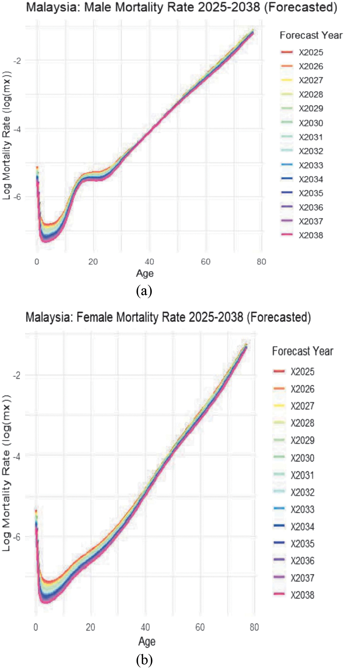Fig. 5. Predicted mortality rates by age and gender, males (a) and females (b), from 2025 to 2038.

The projected mortality curves exhibit only marginal downward shifts over time, as indicated by the narrow gaps between the earlier and later prediction years. This suggests that mortality decline is occurring at a decelerating rate, reflecting a stabilization phase in mortality dynamics. The increase in life expectancy is achieved without substantial shifts in age-specific mortality patterns, as shown in Fig. 6. Such behavior aligns with empirical findings that mortality reductions persist over time but tend to slow as populations reach advanced stages of demographic transition [28].

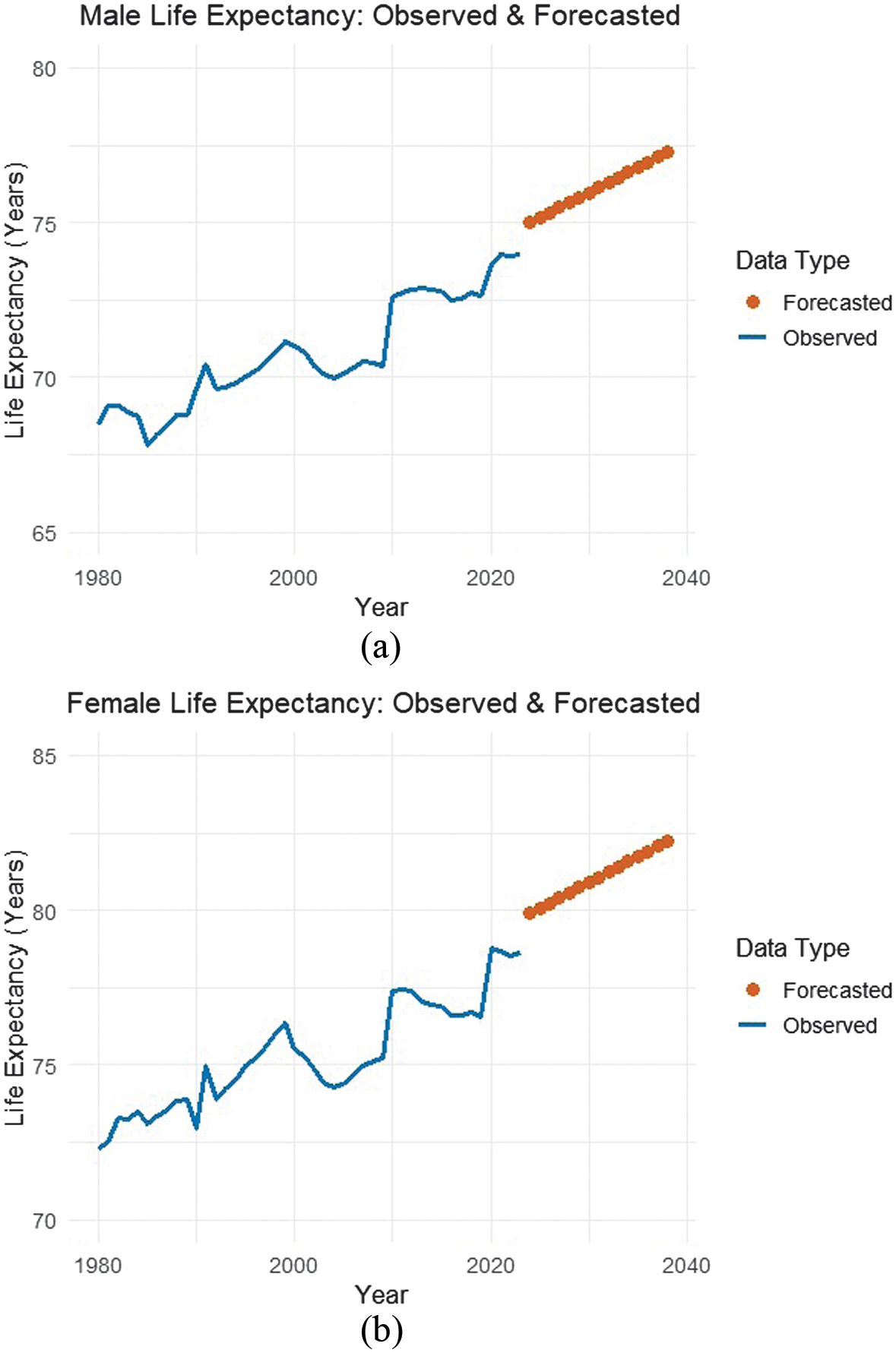Fig. 6. Observed (1980–2024) and projected (2025–2038) life expectancy for Malaysian males (a) and females (b).

Continued slow declines in mortality rates throughout future years lead to a consistent increase in future life expectancy, as depicted in Fig. 6. The projections indicate a gradual and steady rise in life expectancy from 2025 to 2038. Throughout this horizon, females are expected to consistently outlive males, with the life expectancy gap widening to approximately eight years by 2038. These results point to a persistent gender differential in longevity within the Malaysian population.

D.MORTALITY IMPROVEMENT ANALYSIS

Improvements in mortality have practical implications for actuarial work. In particular, premium pricing and reserve calculations can be more accurately aligned with observed and expected longevity patterns, thereby reducing the likelihood of systematic under-pricing or insufficient reserving. More reliable mortality projections also support longer-term planning for pension schemes, which has become increasingly important as Malaysia moves toward an aging population.

The heat map (Fig. 7) illustrates the projected annual improvement rates in female mortality across different age groups and future year intervals. The y-axis represents age, ranging from 0 to 80+ years. The x-axis shows successive biennial year intervals, starting from 2025–2026 to 2037–2038. The color intensity, as indicated by the “Improvement” legend on the right, corresponds to the mortality improvement rate. Darker shades of blue represent higher improvement rates (up to 0.04), while lighter shades indicate lower improvement rates (down to 0.01).

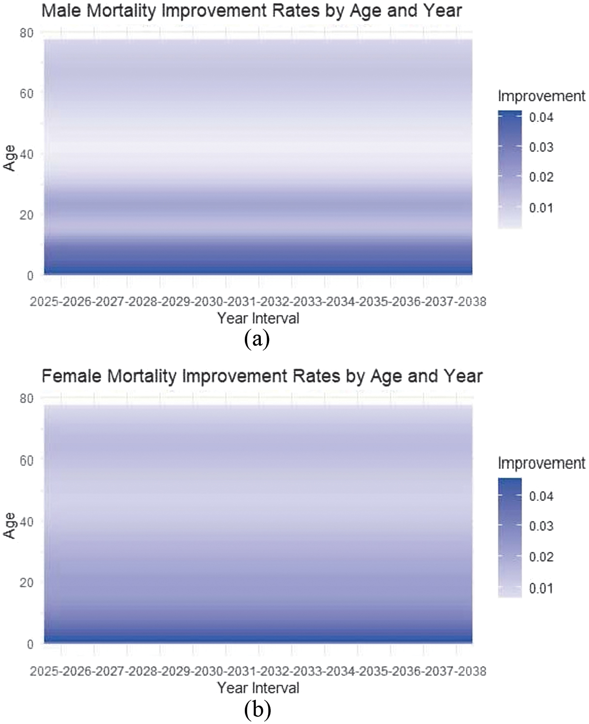Fig. 7. Malaysian mortality improvement rates by age and gender (males (a) and females (b)). Darker shades represent high mortality improvement rates, whereas lighter shades indicate low mortality improvements.

Substantial improvements in mortality are observed among infants and young children, as indicated by the darkest shades at the lower age groups, suggesting that survival at younger ages is expected to continue improving in the future. These developments contribute significantly to long-term gains in life expectancy and further support projections of population aging and increased longevity in Malaysia. In contrast, the least mortality improvement is observed among middle-aged individuals, particularly those aged 40 to 50 years, as shown by the lighter blue shades. This pattern is more pronounced among males compared to females.

V.CONCLUSION AND RECOMMENDATIONS

This study evaluates the optimization of fitting period selection for mortality forecasting in the Malaysian context by comparing the predictive performance of the standard LC model with three extended variants: the LC-ARIMA model and two machine learning-enhanced approaches, LC-ANN and LC-RF. The findings demonstrate that the choice of fitting period plays a critical role in determining forecast accuracy across all models. Using Malaysian mortality data from 1980 to 2024, the results indicate that an appropriately selected fitting period substantially improves predictive performance. In particular, the LC-ANN model achieved the lowest forecast errors for males, with the optimal fitting period identified as 1980–2010. Moreover, when averaged across both genders, LC-ANN consistently outperformed the competing models, especially under longer fitting periods. These results highlight the importance of fitting period optimization and provide empirical support for the integration of machine learning techniques in enhancing mortality forecasting models.

The analysis confirms a sustained decline in mortality over time, with improvements appearing more pronounced and stable among females. Correspondingly, life expectancy is projected to continue increasing through 2038. These findings are especially relevant in Malaysia and other rapidly aging countries, where demographic projections indicate a transition to an aging population. Reliable mortality forecasts are therefore essential for informing insurance pricing, reserving valuation, pension planning, and broader public policy. Future research could extend this study by incorporating more flexible machine-learning and hybrid mortality models, such as deep-learning-based extensions of the LC framework, to better capture nonlinear and cohort-specific patterns.

A Hybrid Lee–Carter Mortality Prediction Framework with Optimized Fitting Period and Machine Learning Integration