JAIT

I.INTRODUCTION

Organizational audit is a systematic activity aimed at evaluating an organization’s strategic development, operational effectiveness, and potential risk factors that may affect its future growth [1,2]. Unlike narrowly focused financial audits, organizational audits assess a wide range of elements, including resources, business processes, policies, information systems, and governance structures, in order to determine their alignment with organizational goals and regulatory requirements. As a result, organizational audits play a critical role in identifying inefficiencies, outdated practices, and latent risks that may hinder an organization’s adaptability in increasingly complex and dynamic business environments.

Modern organizations operate within highly interconnected and data-intensive information systems, where business processes, data flows, and technological infrastructures continuously evolve [3–7]. The growing complexity of enterprise systems, combined with increasing volumes of heterogeneous audit data, has made traditional manual audit procedures progressively less effective. Manual analysis is time-consuming, prone to human error, and difficult to scale, particularly when dozens of risk indicators and cross-sector organizational characteristics must be considered simultaneously. These limitations highlight the need for intelligent, data-driven approaches that support auditors in large-scale, multidimensional risk assessment tasks.

Recent advances in artificial intelligence (AI), particularly machine learning (ML) and deep learning (DL), offer promising opportunities to automate and enhance audit analytics. ML-based techniques have been increasingly adopted for tasks such as fraud detection, risk scoring, document analysis, and compliance monitoring. By leveraging predictive models, auditors can prioritize high-risk entities or documents, thereby improving audit efficiency and allowing experts to focus on critical decision-making tasks. However, the effectiveness of such models strongly depends on data quality, feature selection, and the ability to interpret model outputs in a manner that is meaningful to domain experts.

Despite growing interest in AI-assisted auditing, existing research exhibits several limitations. Most prior studies focus on narrowly defined problems, such as financial fraud detection or cybersecurity audits [8], often within a single domain or data type. Moreover, while advanced ML and DL models can achieve high predictive performance, they are frequently treated as “black boxes,” limiting their practical adoption in audit contexts where transparency, traceability, and accountability are essential. Explainable AI techniques, such as Correlation analysis, Feature Importance measures, and SHapley Additive exPlanations (SHAP), are still underutilized in organizational audit research, particularly in studies involving multi-sector data and comparative model evaluation.

In this context, the present study aims to design and evaluate an intelligent and interpretable organizational audit risk classification framework. The proposed framework integrates data preprocessing, Chi-square-based feature selection, Correlation analysis, and model-based Feature Importance with a comprehensive set of ML and DL classifiers, including random forest (RF), XGBoost, dense neural networks (DNNs), and hybrid recurrent architectures such as long short-term memory (LSTM)-gated recurrent unit (LSTM-GRU). SHAP-based explainability is employed to provide both global and local interpretations of model predictions, supporting transparency and informed human-in-the-loop audit decision-making. Rather than proposing new algorithms, this work focuses on systematically integrating and evaluating these techniques within a unified audit analytics pipeline.

The main contributions of this study can be summarized as follows:

−A comprehensive comparison of traditional ML and DL models for organizational audit risk classification using a real-world, multi-sector dataset.
−A structured feature selection and analysis process that combines statistical methods (Chi-square and Correlation analysis) with model-driven Feature Importance and SHAP explanations.
−An extensive evaluation framework that considers predictive performance, calibration, computational efficiency, and interpretability, addressing practical deployment concerns in audit environments.
−An interpretable audit decision-support pipeline that enhances transparency while preserving strong classification performance.

The remainder of this paper is organized as follows. Section II reviews related work on AI-based auditing and risk assessment. Section III describes the dataset, preprocessing steps, feature selection procedures, and model architectures. Section IV presents experimental results and performance analysis. Section V discusses the findings, limitations, and practical implications and outlines directions for future research.

II.LITERATURE REVIEW

There are numerous papers on ML and DL approaches to data auditing.

The paper [9] explores information security concepts and the methods for managing the latest security threats, drawing on guidance from experts and advisors. The paper [10] examines the effectiveness of auditing the financial transactions of Chinese companies and reporting on fraudulent activities using several ML algorithms, such as logistic regression (LR) [11], support vector machine (SVM) [12], RF [13], AdaBoost, XGBoost, and RUSBoost. The RUSBoost algorithm shows the best results, achieving classification accuracy values of 0.721. Reference [14] analyzes and predicts audit results in municipalities of South Africa. The dataset includes 1560 financial observations from entity reports, 55% of which are unqualified audit opinions. The accuracy of classification models is assessed using LR, decision tree (DT), and artificial neural networks (ANNs). The ANN model achieves the receiver operating characteristics (ROC) values of 0.71 and 0.74 with the entire feature set.

In ref. [15], supply efficiency is considered in the study of waste management for sustainable development and cost reduction. The neural network (NN) model achieves F1-scores of 0.72 and 0.71. The study [16] uses DT, Bayesian belief network (BBN), and other NNs. It analyzes data from the financial statements of Greek organizations, including their profit and loss statements. At the same time, the BBN model shows the best results in classifying companies with a prediction accuracy of 90.3%. The accuracy score is 80% for the NN and 73.6% for the DT models. In ref. [17], capital turnover and fraudulent financial reporting are investigated using publicly available data from 103 and 100 firms over a 2-year period. The LR algorithm shows the best classification results. In ref. [18], the authors propose using ML models in document management systems, where documents scanned for audit are processed using information retrieval and content recognition techniques, achieving an accuracy of 0.93 or higher. The paper [19] describes the implementation of the DT model for analyzing financial indicators. The accuracy of the model’s prediction in the financial sector is around 93%. In ref. [20], the ML approach is used to evaluate the risk assessments of the supplement chains, reducing the subjectivity of the main user analysis. The estimated risk probability reaches 87%. The authors of ref. [21] explore the business characteristics of organizations, such as size, profitability, and sustainability, using regression and ML models. They found that these factors are the most critical for estimating the efficiency of business organizations. Many more works and research publications explore and evaluate the audit of organizations. A comparative overview of the most relevant ML/DL-based auditing studies, including applied models, domains, performance, and limitations, is presented in Table I.

Table I. Comparative analysis of ML/DL applications in audit-related tasks

Study	ML/DL methods	Dataset/domain	Best result	Limitation
J. Brasse et al. [10]	LR, SVM, RF, AdaBoost, XGBoost, RUSBoost	Financial transactions (China)	RUSBoost, accuracy = 72.1%	Focused only on imbalanced fraud data
Mabelane et al. [13]	LR, DT, ANN	1560 municipal audit reports (South Africa)	ANN, ROC = 0.74	Public sector only
Kirkos et al. [16]	DT, BBN, NN	Greek financial statements	BBN, accuracy = 90.3%	Narrow financial domain
Persons [17]	Logistic regression	US firms, 2-year turnover data	—	The traditional method only
Othmane et al. [18]	ML + IR + OCR	Audited scanned documents	Accuracy > 93%	No DL/SHAP interpretation
Xiaofeng et al. [22]	Deep learning	Financial auditing logs	Enhanced performance	No explainability tools
The present study	RF, XGBoost, DNN, CNN-LSTM, LSTM-GRU	773 organizational units across 14 sectors	Accuracy = 0.957, F1 = 0.958	First to use SHAP + hybrid DL + multi-sector data

The reviewed literature confirms the successful application of ML and DL methods in various audit-related tasks, particularly in financial auditing and document classification. However, several important gaps remain:

•Most studies are domain-specific and do not generalize across organizational types or sectors.
•The majority of works rely on traditional ML methods, with limited exploration of hybrid or deep neural architectures.
•Explainability techniques such as SHAP or feature attribution analysis are rarely applied, reducing trust in model outputs.

This study addresses these limitations by introducing a hybrid framework that combines interpretable ML and DL models, feature selection, and multi-sector risk indicators. It is one of the first to integrate SHAP, Feature Importance, and Correlation analysis into an intelligent organizational audit pipeline.

III.METHODOLOGY

This paper discusses the construction of ML [22] and DL [23] models for determining the risks of organizations. The model development stages encompass the following steps: dataset preparation, data normalization, feature selection, and classification using ML and DL models [24]. The entire methodology is illustrated in Fig. 1.

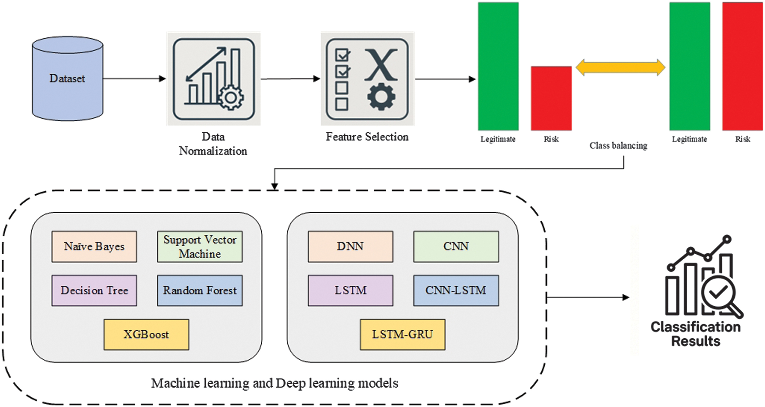Fig. 1. The methodological scheme of data processing and classification with ML and DL models.

The organizational audit dataset, comprising 773 units (305 risky and 468 non-risky organizations), is sourced from the GitHub website [25]. This dataset consists of 26 features describing the risk parameters for 14 types of organizations: Corporate, Communications, Buildings and Roads, Science and Technology, Public Health, Irrigation, Forest, Animal Husbandry, Electrical, Land, Tourism, Industries, Fisheries, and Agriculture. In the study, auditors visited companies’ offices and examined their business activities. The audit processes include the following specifications:

−Interviewing employees and proposing risk assessments of organizations.
−Investigating the entire history of various risk factors to examine and evaluate the degree of risk of the analyzed organizations.
−Implementing the particle swarm optimization algorithm to improve the ranking of risk factors and evaluate the organization’s risk class (fraudulent and non-fraudulent).

In the dataset, the “Audit_Risk” feature is derived from the “Risk” label, suggesting a direct dependence between this feature and the outcome. The label is called “Risk” and is already presented in a binary (0/1) format. The detailed description of all 26 features is shown in Table II.

Table II. The description of the dataset features

No.	Feature name	Definition	Data type	Unit	Derivation from label
1	Sector_score	Risk weight assigned to the industrial sector of the organization based on regulatory vulnerability	Continuous	Index	No
2	LOCATION_ID	Encoded geographical location identifier of the organization	Categorical	None	No
3	PARA_A	Regulatory compliance violations	Continuous	Count/score	No
4	Score_A	Normalized score derived from PARA_A	Continuous	Index	No
5	Risk_A	Risk class derived from Score_A	Categorical	Low/medium/high	No
6	PARA_B	Financial irregularities	Continuous	Count/score	No
7	Score_B	Normalized score derived from PARA_B	Continuous	Index	No
8	Risk_B	Risk class derived from Score_B	Categorical	Low/medium/high	No
9	TOTAL	Aggregate audit parameter score across A and B categories	Continuous	Index	No
10	numbers	Operational scale indicator	Discrete	Count	No
11	Score_B.1	Secondary normalized score derived from TOTAL	Continuous	Index	No
12	Risk_C	Risk category derived from Score_B.1	Categorical	Low/medium/high	No
13	Money_Value	Total audited financial turnover of the organization	Continuous	Currency	No
14	Score_MV	Normalized financial exposure score derived from Money_Value	Continuous	Index	No
15	Risk_D	Financial risk class derived from Score_MV	Categorical	Low/medium/high	No
16	District_Loss	Financial loss recorded at the district level	Continuous	Currency	No
17	PROB	Expert-estimated probability of loss occurrence	Continuous	Probability [0–1]	No
18	RiSk_E	Economic environment risk index	Continuous	Index	No
19	History	Binary indicator of prior audit violations	Binary	[0,1]	No
20	Prob	Historical probability of previous audit failures	Continuous	Probability [0–1]	No
21	Risk_F	Final probabilistic risk category	Categorical	Low/medium/high	No
22	Score	Global aggregated risk score computed from all sub-scores	Continuous	Index	No
23	Inherent_Risk	Intrinsic organizational risk before controls	Continuous	Index	No
24	CONTROL_RISK	Risk remaining after internal control measures	Continuous	Index	No
25	Detection_Risk	Risk of audit failure to detect anomalies	Continuous	Index	No
26	Audit_Risk	Evaluation of the risky or non-risky degree	Continuous	Probability	YES

All significant risk factors are identified through interviews, and their likelihood of existence is assessed. The external auditors evaluate the discrepancies and misstatements of the organization’s financial documents, including fraud factors and other errors. The risk is usually measured as the expected value of the undesirable outcome, such as the likelihood of material misstatements in the financial statements, using an audit risk assessment (ARA). This organizational audit dataset includes the following features, defining the risk factors of organizations: para (the inconsistency found in the planned expenses of inspection), number (the historical inconsistency score), sector score (the historical risk score in a specific sector of the organization), history (an average historical loss of the organization), money (the sum of money implemented in past misstatements), etc.

The distribution by class is shown in Fig. 2.

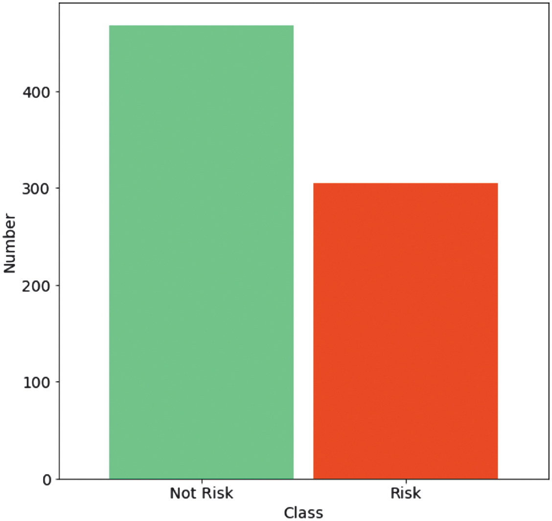Fig. 2. The distribution of risk and not risk units into corresponding classes.

The dataset’s features generally do not contribute equally to the essential factors, especially when their number exceeds several dozen. Therefore, it is preferable not to use all of them during ML model training but to select the most important ones, accepting the associated inaccuracies. In this way, the specialized normalization techniques are reflected in the preparation of optimal features for the dataset used. Among these techniques, the most popular ones are the mean and min-max scaling methods.

Mean normalization [26] is calculated by Eq. (1):

| a | = \frac{a - \bar{a}}{\max (a) - \min (a)}

(1)

where

\bar{a}

is a mean value,

a

is an initial value, and

| a |

is a normalized value.

Min-max normalization [27] is calculated by Eq. (2):

| a | = \frac{a - \min (a)}{\max (a) - \min (a)}

(2)

where

| a |

is a normalized value and

a

is an initial value. The min-max method is used to conduct the experimental results.

There are infrequent occasions when all the features must be used during the development of ML models. Therefore, feature selection techniques are used to reduce the dataset’s dimensionality significantly. There are many feature selection techniques used in dataset processing. They are even divided into several categories: Filter (Chi-square, Mutual Information, Correlation, and Information Gain), Wrapper (Stepwise Selection, Backward Elimination, and Forward Selection), and Embedded (Lasso, Ridge Regression, and Elastic Net).

Information Gain [28] considers the Correlation of objective functions according to the reduction of the data transformation’s entropy. It selects features by measuring the values of every variable. It is calculated by Eq. (3):

I (X; Y) = H (Y) - H (Y | X)

(3)

The Chi-square test [27] computes the score of each feature by comparing observed and expected values and identifying the features that show the best scores. It is calculated by Eq. (4):

s_{c}^{2} = \sum \frac{{(X_{i} - Y_{i})}^{2}}{Y_{i}}

(4)

where

X

is observed values,

Y

is expected values, and

s_{c}

is a score.

Mutual Information [29] is a model-agnostic feature selection technique that measures the statistical dependency between an input feature and a target variable. It originates from information theory and quantifies how much information knowing one variable provides about another. It is calculated by Eq. (5):

M I (X, Y) = \sum_{x \in X} \sum_{y \in Y} p (x, y) l o g \frac{p (x, y)}{p (x) p (y)}

(5)

In the experimental results presented in this paper, the Chi-square test is employed for feature selection. The additional comparative experiments are conducted with the use of Mutual Information.

The selected features are evaluated with the use of Feature Importance, Correlation heatmap, and SHAP summary [30] metrics.

Feature Importance is a technique in ML used to determine which input features have the most influence on a model’s predictions. It provides a ranking or score that reflects the usefulness or value of each feature in building the model. This concept is especially useful for understanding complex models and improving their interpretability. In this research, XGBoost is used for calculating the Feature Importance.

A Correlation heatmap is a graphical representation of the Correlation matrix between multiple variables in a dataset. It visually displays the strength and direction of linear relationships between pairs of features using color gradients. Typically, the values range from −1 to 1, where 1 indicates a perfect positive Correlation, −1 a perfect negative Correlation, and 0 no Correlation at all. In the heatmap, rows and columns represent the features, and the intersecting cell color encodes the Correlation value—darker or more intense colors usually indicate stronger Correlations.

A SHAP summary [31] plot is a visualization that provides a comprehensive overview of how features affect a model’s predictions, based on SHAP ions values. It combines both Feature Importance and feature effect into a single, interpretable chart. In this plot, each dot represents a SHAP value [32] for an individual data point and a specific feature. The x-axis represents the SHAP value, indicating the extent to which a feature contributes to increasing or decreasing the model’s prediction. The y-axis lists the features, ordered by overall importance—features at the top are the most influential. The color of each dot reflects the original feature value (e.g., red for high values and blue for low values), allowing users to understand how specific values affect predictions.

The class balancing technique [33] is implemented to avoid severely penalizing model performance due to false-negative predictions. The Random Oversampling method is chosen for class balancing. This method works by randomly duplicating samples from the minority class until the number of samples in each class becomes approximately equal. Unlike undersampling, Random Oversampling does not remove any majority-class samples, thereby preserving all available information from the dominant class. Random Oversampling is shown in Fig. 3.

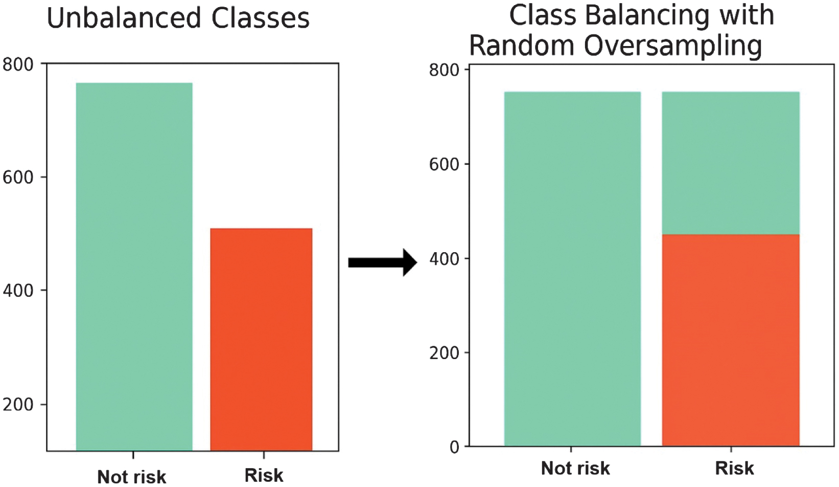Fig. 3. Class balancing technique for risk and not risk units.

After the best features are chosen, the dataset is further classified with several ML and DL models: Naive Bayes (NB), SVM, DT, RF, XGBoost, DNN, convolutional neural network (CNN), LSTM, CNN-LSTM, and LSTM-GRU.

The choice of ML and DL models [34] has to consider various factors. Classical ML models, such as NB, SVM, and DT, are highly interpretable and computationally inexpensive but exhibit lower predictive accuracy. RF and XGBoost ensemble methods provide a balance between predictive power and interpretability, with fast inference, modest resource requirements, and compatibility with SHAP-based explanations. DNN, CNN, LSTM, CNN-LSTM, and LSTM-GRU DL models introduce significantly greater model complexity, longer training times, and limited interpretability, while yielding only marginal, non-statistically significant improvements relative to ensemble methods. From the perspective of real-world audit deployment, where explainability, reliability, and low-latency decision support are essential, such complexity offers limited practical advantage. Accordingly, RF and XGBoost emerge as effective and parsimonious candidates, combining strong performance with operational feasibility and interpretable behavior suitable for audit triage and risk assessment workflows.

NB [28] is a straightforward ML algorithm that is based on the probabilistic approach. It is calculated by Eq. (6):

P (D | C) = \frac{P (D) \times P (C | D)}{P (C)}

(6)

where

P (D)

is an observed probability,

P (C)

is an occurred probability, and

P (C | D)

is a probability that a feature is classified as a label.

SVM [14] is an algorithm that works with a space of features shared by a separation hyperplane, having the greatest distance to the nearest points of the training data of two classes.

The hyperplane equation is calculated by Eq. (7):

y_{i} (\vec{w} \times \vec{x} + b) \geq 0

(7)

where

\vec{w} = (w_{1}, w_{2}, \dots, w_{n})

is a vector of weights,

\vec{x} = (x_{1}, x_{2}, \dots, x_{n})

is a feature vector,

y_{i}

is an output value, and

b

is bias. The hyperplane is shown in Fig. 4.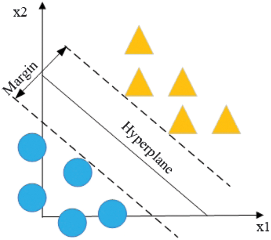

Fig. 4. Illustration of a support vector machine (SVM) separating hyperplane [10].

DT [16] is an algorithm that uses a method based on dividing a dataset by features, answering specific questions until all data points belong to a particular class. Thus, a tree structure is formed by adding a node for each question (Fig. 5).

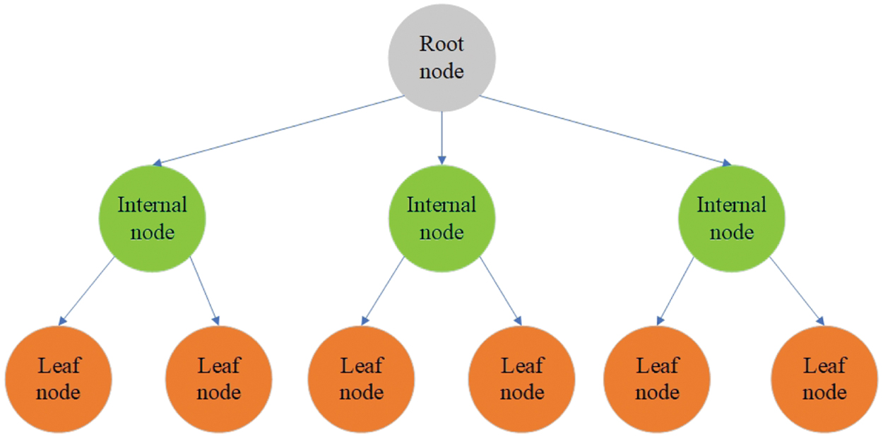Fig. 5. Illustration of the decision tree classifier [11].

RF [18] uses the concept of ensemble learning, involving several classifiers for the improvement of the performance of the ML model. This algorithm includes a range of DTs. The class is defined by the highest number of votes of all trees in the ensemble (Fig. 6).

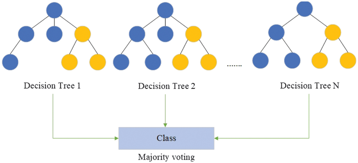Fig. 6. Illustration of the random forest ensemble classifier [11].

XGBoost [20] is an advanced ML algorithm that uses the boosting principle. The preceding errors are eliminated in a new model using the boosting approach, and the deviations of the trained ensemble predictions are calculated on the training set at every iteration. Therefore, the optimization is performed by adding new tree predictions to the ensemble, dropping the mean deviations.

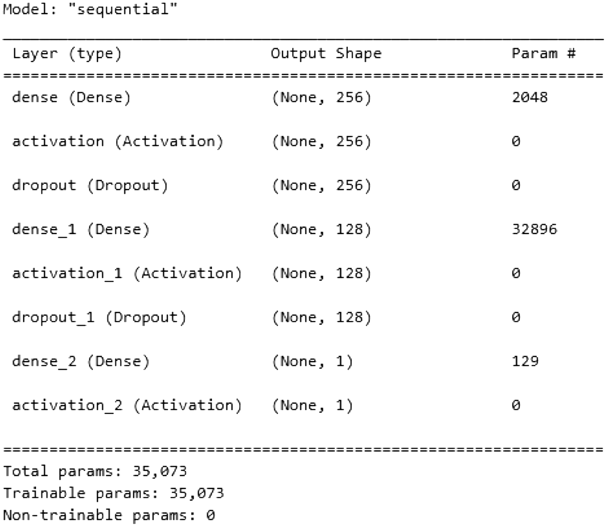
DNN [22] is a model of NN with two or more hidden layers. A DNN consists of an input layer containing the input data, hidden layers containing nodes called neurons, and an output layer comprising one or more neurons (Fig. 7).

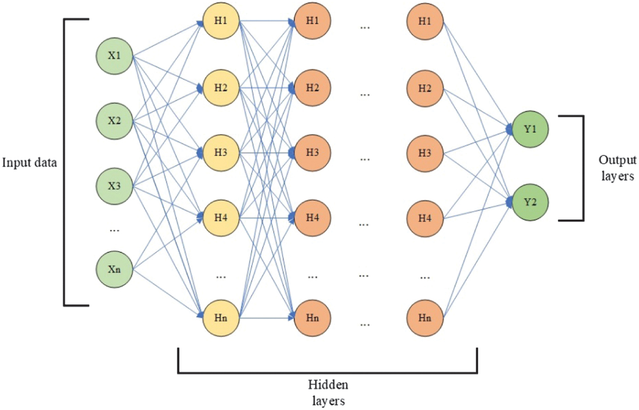Fig. 7. The architecture of a dense neural network [26].

The hyperparameters of ML models are shown in Table III.

Table III. Hyperparameters of ML models

Model	Hyperparameter	Value used
Multinomial Naive Bayes	Alpha	1.0
	fit_prior	True
Support vector machine	Kernel	linear
	C	1.0
	Gamma	scale
Decision tree	Criterion	gini
	Splitter	best
	max_depth	None
Random forest	n_estimators	10
	Criterion	gini
	max_depth	None
	Bootstrap	True
XGBoost	random_state	42
	learning_rate	0.3
	max_depth	6
	n_estimators	100
	Subsample	1.0

In the DNN, $x = x_{1}, x_{2}, \dots, x_{f}$ is an input vector, $w_{1}, w_{2}, \dots, w_{i}$ are weights, $b_{1}, b_{2}, \dots, b_{i}$ is a bias vector, and $y_{1}, y_{2}, \dots, y_{m}$ is an output vector. The structure of the network used in the experiments contains one input layer, two hidden layers, two dropout layers, and one output layer. The hyperparameters of DNN are shown in Table IV.

Table IV. Hyperparameters of DNN

Category	Parameter	Value used
Architecture	Hidden layers	256–128
	Activation	ReLU/Sigmoid
	Dropout	0.4/0.2
	L2 regularizer	1e–4
Optimization	Optimizer	Adam
	Learning rate	0.001
Training	Batch size	14000
	Epochs	100
	Validation split	0.125
	Early stopping	Not used
Loss and metrics	Loss	Binary cross-entropy
	Metrics	Accuracy, precision, recall, F1-score

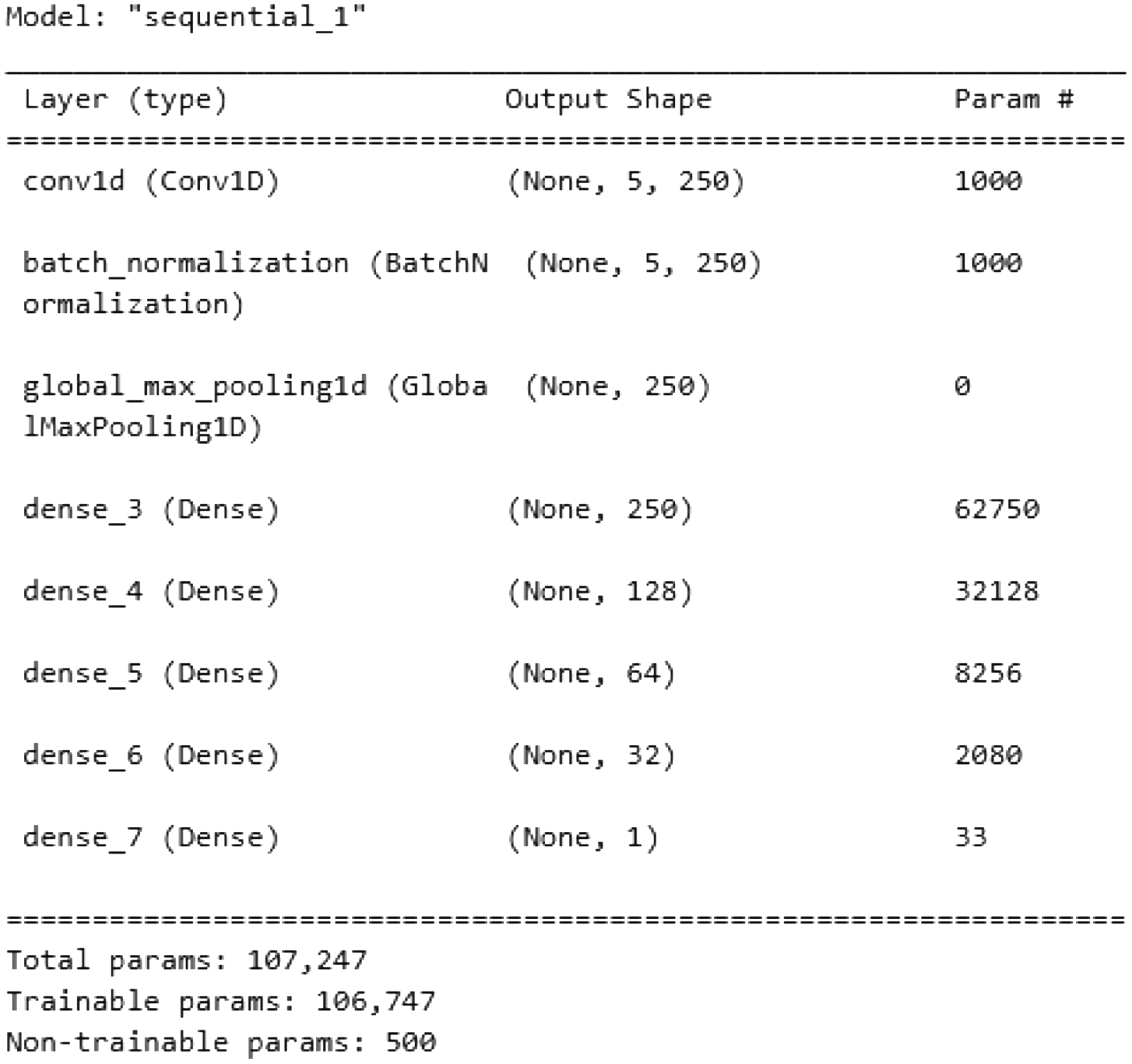
CNN [23] is a type of NN that processes spatially structured input data, such as images and videos, and can also efficiently handle text data represented as a one-dimensional vector. The architecture of this NN includes the following elements:

−A convolutional layer is a layer that performs a convolution of the input data using a filter. The filter moves over an image or text vector using convolution operations.
−A max-pooling layer is a layer that reduces feature size by selecting the maximum value within a given region.
−An output layer is a layer that contains the results of binary classification. In this binary classification problem, the vector represents the output values $\vec{y} = y_{1}, y_{2}$ of the CNN as shown in Fig. 8.

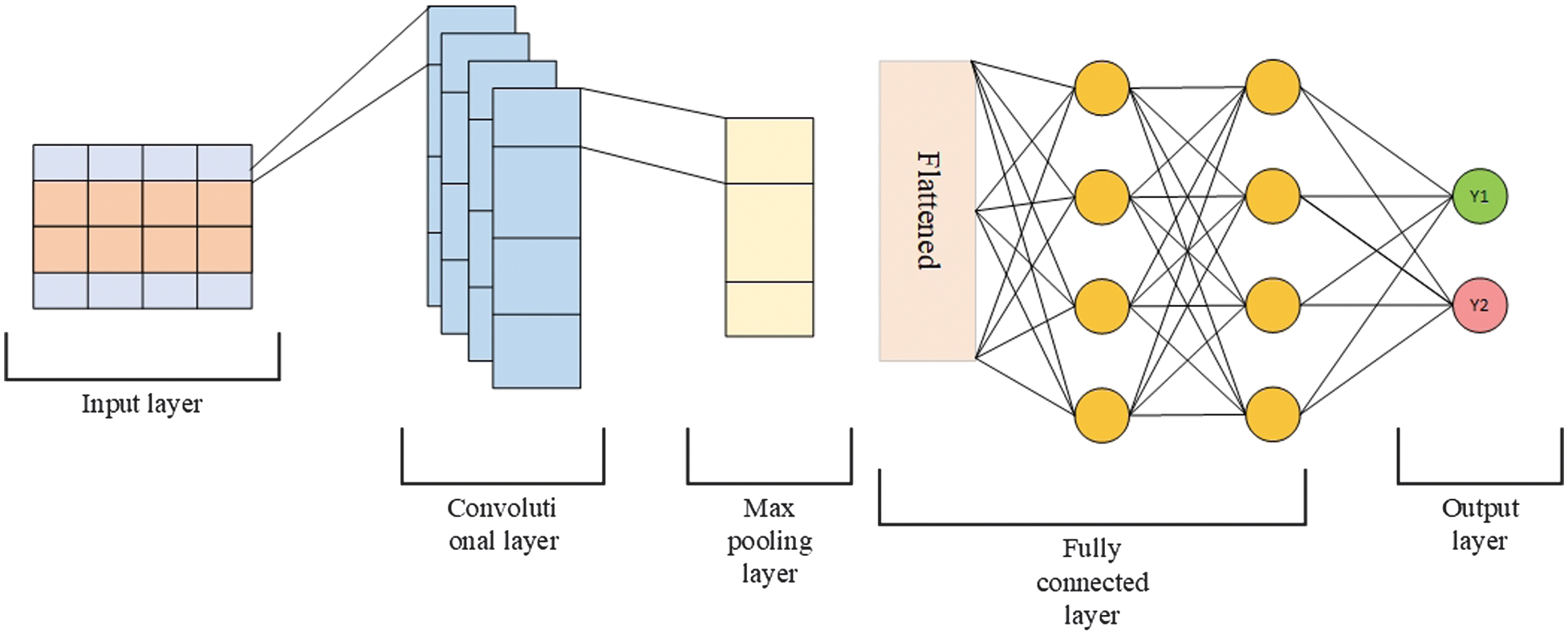Fig. 8. The architecture of a convolutional neural network.

The hyperparameters of the CNN are shown in Table V.

Table V. Hyperparameters of CNN

Category	Parameter	Value used
Convolution	Filters	nb_filter
	Kernel size	filter_length
	Activation	ReLU
	L2 regularizer	1e-4
Pooling	Pooling type	Global Max Pooling
Dense layers	Fully connected layers	hidden_dims, 128, 64, 32
Optimization	Optimizer	Adam
	Learning rate	0.00008
Training	Batch size	14000
	Epochs	100
	Validation split	0.125
	Early stopping	Not used
Loss and metrics	Loss	Binary cross-entropy
	Metrics	Accuracy, precision, recall, F1-score

LSTM [24] is a type of recurrent neural network (RNN) designed to process sequential data and take context into account across different sequences. LSTM mandatory has the following elements:

−A memory cell $C_{t - 1}$ is the memory cell at the previous time step. It represents the information that is saved in the previous steps.
−A memory cell $C_{t}$ is a state of the current memory cell. It is updated based on the previous memory cell, the input data $x_{t}$ , and the forget and input gates that determine what information to keep or forget.
−A previous state $h_{t - 1}$ is a hidden state at the previous time step.
−A state $h_{t}$ is a current hidden state.
−Data $x_{t - 1}$ are input data from the previous time step.
−Data $x_{t}$ are input data at the current time step.

LSTM is shown in Fig. 9.

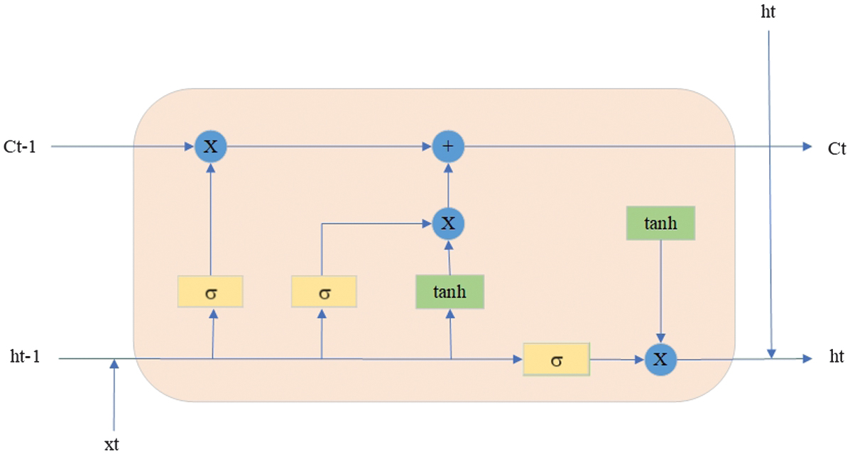Fig. 9. The architecture of a long short-term memory neural.

The hyperparameters of LSTM are shown in Table VI.

Table VI. Hyperparameters of LSTM

Category	Parameter	Value used
Recurrent layers	LSTM units (layer 1)	128
	LSTM units (layer 2)	32
	Return sequences	True
	L2 regularizer	1e-4
Regularization	SpatialDropout1D	0.2
	Dropout	0.2
Output layer	Activation	Sigmoid
Optimization	Optimizer	Adam
	Learning rate	0.0001
Training	Batch size	14000
	Epochs	100
	Validation split	0.125
	Early stopping	Not used
Loss and metrics	Loss	Binary cross-entropy
	Metrics	Accuracy, precision, recall, F1-score

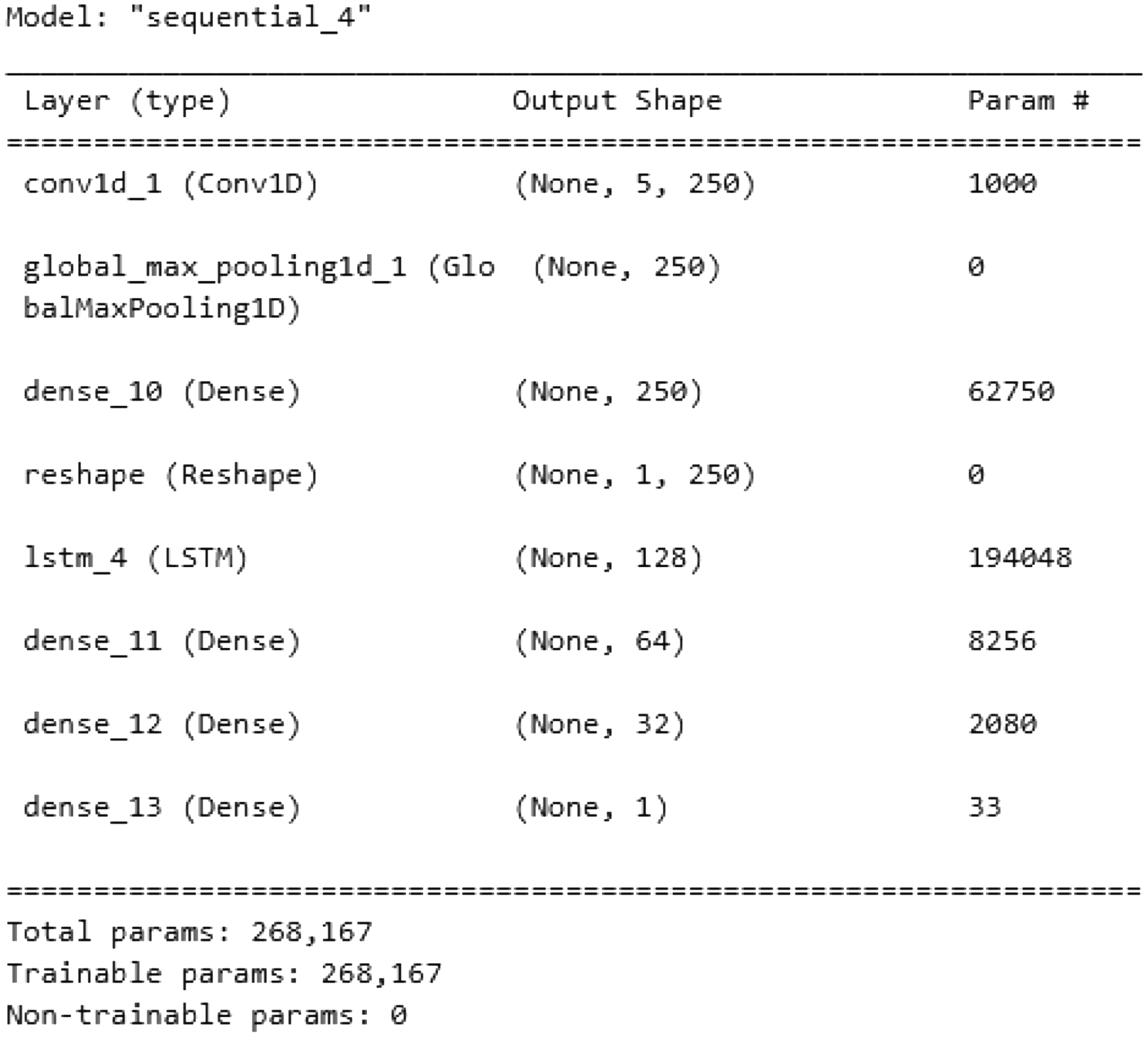
The CNN-LSTM neural network is a hybrid architecture that combines a CNN and an LSTM to process data with both spatial and temporal characteristics effectively. This model is particularly suited to tasks where both local feature extraction and sequence modeling are crucial [35]. The CNN-LSTM model detects complex patterns across various features. The CNN component serves as a feature extractor. It scans the input using convolutional filters to capture local dependencies or spatial structures, such as edges in images, frequency patterns in signals, or n-gram features in text. Once spatial features are extracted, they are reshaped and passed into the LSTM component, which is adept at learning temporal dependencies. The LSTM network processes the sequential nature of the data by maintaining a form of memory over time steps. Combining CNN and LSTM layers creates a powerful end-to-end model capable of jointly learning spatial structures and temporal sequences. CNN-LSTM is shown in Fig. 10. The structure of the model is presented in Table VII.

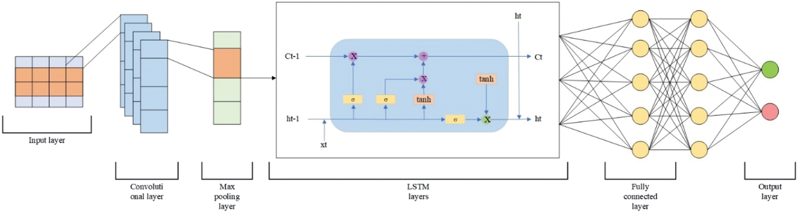Fig. 10. The architecture of a CNN-LSTM.

Table VII. The hyperparameters of CNN-LSTM

Category	Parameter	Value used
CNN block	Filters	nb_filter
	Kernel size	filter_length
	Activation	ReLU
	Pooling	Global Max Pooling
	Dense after CNN	hidden_dims
	L2 regularizer	1e-4
Reshaping	Reshape target	(1, hidden_dims)
LSTM block	LSTM units	128
	Return sequences	False
Fully connected	Dense layers	64 – 32
Optimization	Optimizer	Adam
	Learning rate	0.0001
Training	Batch size	14000
	Epochs	100
	Validation split	0.125
	Early stopping	Not used
Loss and metrics	Loss	Binary cross-entropy
	Metrics	Accuracy, precision, recall, F1-score

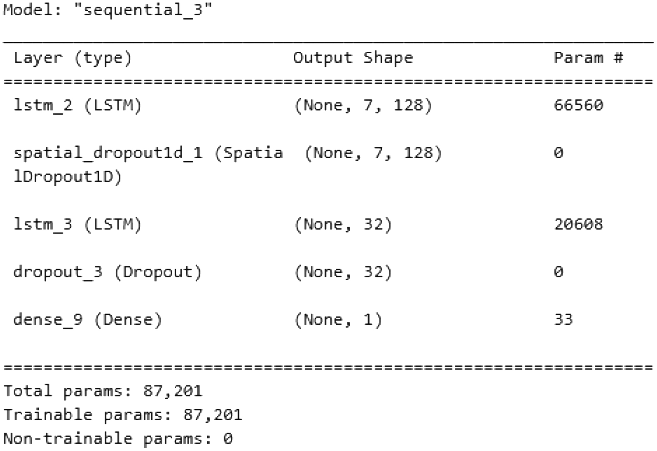
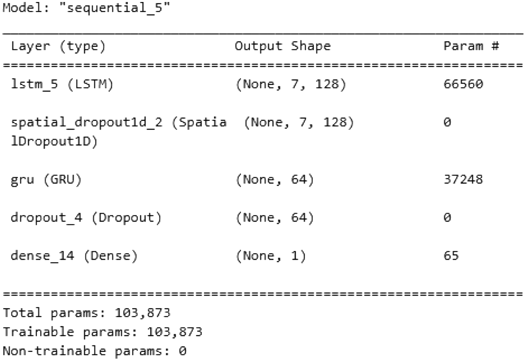
The LSTM-GRU model is a hybrid NN architecture that integrates both LSTM and GRU layers [36]. These two types of RNNs are widely used for processing sequential data such as time series, natural language, or speech. By combining them, the LSTM-GRU model aims to take advantage of the strengths of both architectures to improve performance on complex tasks. LSTM layers are particularly effective at learning long-term dependencies within sequences, thanks to their three-gate structure: input, forget, and output gates. GRU layers use a simplified gating mechanism with only reset and update gates [37]. This makes GRUs more computationally efficient, often resulting in faster training and inference while still performing well on many tasks. The hybrid model leverages the memory capacity of LSTM and the speed and simplicity of GRU to capture both long- and short-term patterns effectively. LSTM-GRU is shown in Fig. 11. The structure of the model is presented in Table VIII.

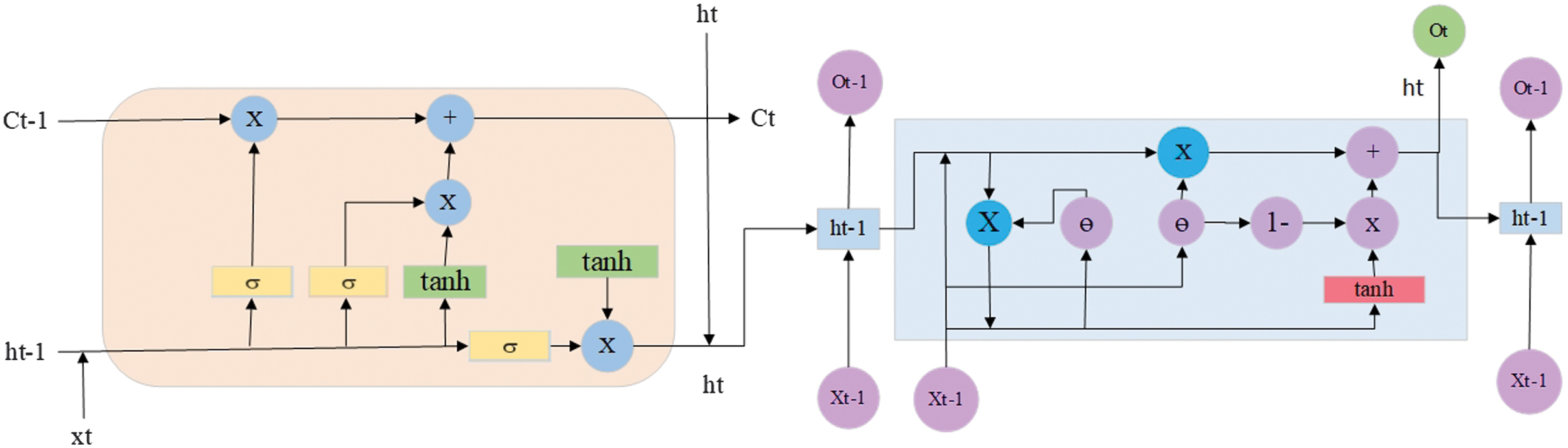Fig. 11. The architecture of an LSTM-GRU.

Table VIII. The structure of the LSTM-GRU neural network

Category	Parameter	Value used
Recurrent block (LSTM)	LSTM units	128
	Return sequences	True
	L2 regularizer	1e-4
Regularization	SpatialDropout1D	0.25
Recurrent block (GRU)	GRU units	64
Regularization	Dropout	0.2
Output layer	Activation	Sigmoid
Optimization	Optimizer	Adam
	Learning rate	0.0001
Training	Batch size	14000
	Epochs	100
	Validation split	0.125
	Early stopping	Not used
Loss and metrics	Loss	Binary cross-entropy
	Metrics	Accuracy, precision, recall, F1-score

IV.RESULTS AND DISCUSSION

The experiments are conducted on a PC equipped with a Core i7 4790 K CPU, an RTX 2070 GPU, 32 GB DDR3 RAM, a 1 TB SSD, and a 2 TB HDD.

At the first step, the dataset is preprocessed and normalized using the min-max method. Then, the Chi-square feature selection technique is implemented to retrieve the 10 most significant features, and Mutual Information is used to obtain the 14 most important features, respectively. The features are additionally evaluated with the Correlation heatmap, Feature Importance, and SHAP summary.

A Correlation heatmap is a visual tool that summarizes and interprets the strength and direction of relationships between features in a dataset. It displays the pairwise Correlation coefficients between features in the form of a colored matrix. Each cell represents the Correlation between two features, typically measured using Pearson’s Correlation coefficient, which ranges from −1 to +1. A value of +1 indicates a strong positive Correlation: when one variable increases, the other also increases. A value of −1 indicates a strong negative Correlation: as one variable increases, the other decreases. A value of 0 indicates no Correlation, where there is no linear relationship between the variables. For the Chi-square feature selection technique, 10 features are chosen for Correlation analysis.

The Correlation heatmap for Chi-square feature selection is shown in Fig. 12.

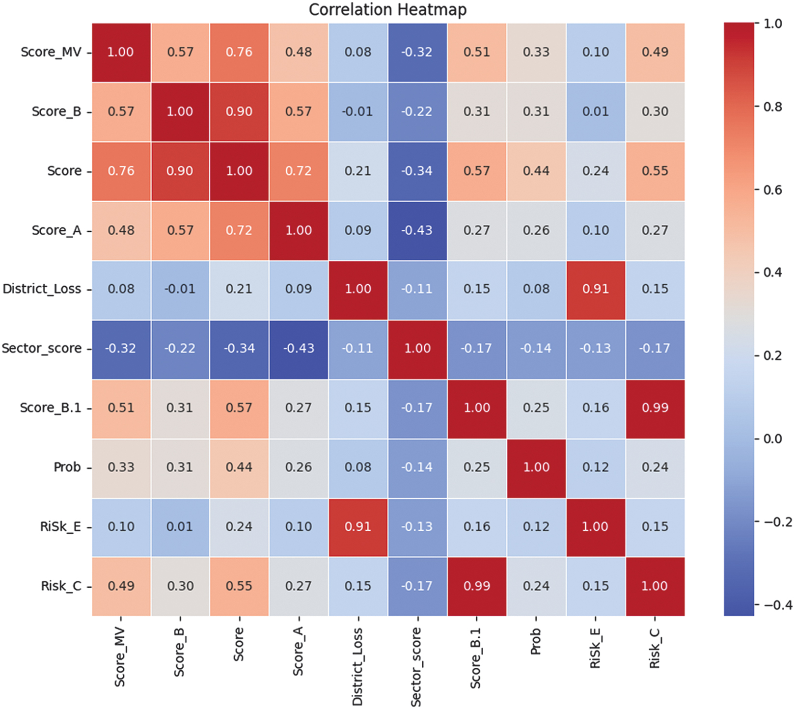Fig. 12. The Correlation heatmap diagram for Chi-square feature selection with 10 features.

This Correlation heatmap shows a very strong positive Correlation of 0.90 between Score and Score_B, as well as 0.99 between Score_B.1 and Risk_C, and 0.91 between District_Loss and RiSk_E, indicating that these features likely carry overlapping or redundant information. High Correlation between these features suggests they could be removed to reduce multicollinearity. On the other hand, features like Sector_score show negative Correlation values −0.43 and −0.34 with Score_A and Score, implying an inverse relationship. Solving a strong Correlation problem, Score_B.1 is removed in favor of Risk_C, Score is eliminated in favor of Score_B, and District_Loss is withdrawn in favor of RiSk_E. A new Correlation heatmap with seven features left is shown in Fig. 13

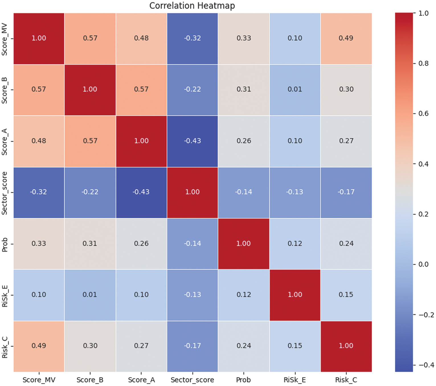Fig. 13. The Correlation heatmap diagram for Chi-square feature selection with 7 features left.

The Correlation heatmap for Mutual Information feature selection is shown in Fig. 14.

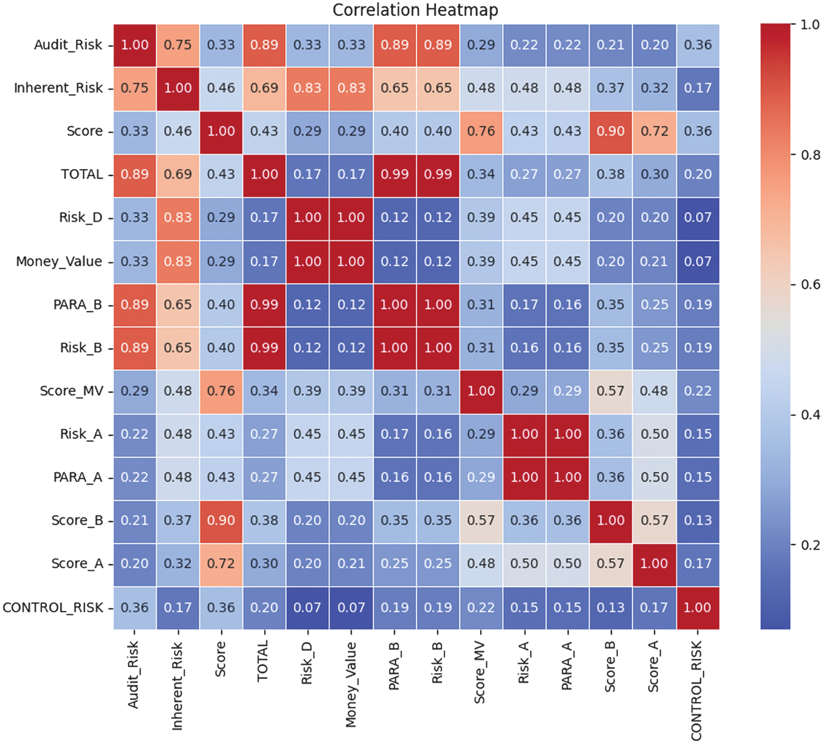Fig. 14. The Correlation heatmap diagram for Mutual Information feature selection with 14 features.

The Correlation analysis, performed after Mutual Information feature selection, reveals that several initially selected variables are highly redundant. As shown in the first Correlation heatmap, multiple feature pairs exhibit robust Correlations of 0.99–1.00, such as Risk_D-Money_Value, PARA_B-Risk_B, and PARA_A-Risk_A, indicating that these variables contain nearly identical information. In addition, composite indicators such as TOTAL, Audit_Risk, and Inherent_Risk show strong Correlations with several base risk and score variables, suggesting overlapping representations of the same underlying risk factors. To address redundancy, a Correlation-based pruning step is applied, retaining only one representative feature from each highly correlated group, prioritizing variables with higher Mutual Information scores and greater interpretability. As a result, the reduced feature set exhibits only low-to-moderate inter-feature Correlations, with a maximum Correlation of 0.57. It confirms that redundant variables are successfully removed while preserving the most informative and complementary risk indicators for subsequent modeling. A new Correlation heatmap with seven features left is shown in Fig. 15.

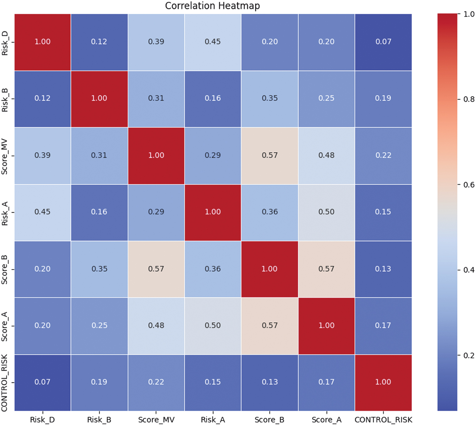Fig. 15. The Correlation heatmap diagram for Mutual Information feature selection with 7 features left.

After the Correlation analysis, the Feature Importance is implemented. Feature Importance is a set of techniques used to quantify the contribution of individual input features to a predictive model’s output. Its primary purpose is to identify which features most strongly influence model decisions, thereby improving interpretability, supporting feature selection, and aiding model validation, especially in high-stakes domains such as auditing and risk assessment. The Feature Importance plot of histograms for seven features of the dataset is shown in Fig. 16.

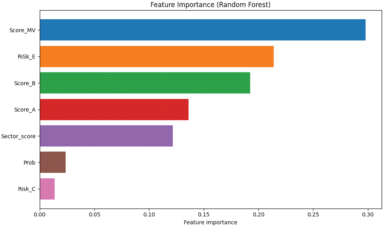Fig. 16. The Feature Importance histograms for 7 features of the dataset.

The Feature Importance plot indicates a clear dominance of a small subset of features in driving audit risk classification. Score_MV emerges as the most influential feature, contributing the largest share to the model’s predictive decisions, followed by Risk_E and Score_B, which also exhibit substantial importance. These features consistently appear as primary split variables within the ensemble, suggesting that they capture critical aspects of organizational risk behavior. Score_A and Sector_score provide moderate contributions, indicating that sector-level context and auxiliary scoring information add incremental predictive value beyond the core risk indicators. In contrast, Prob and Risk_C are of minimal importance, suggesting limited marginal benefit in the presence of stronger predictors. Overall, the results demonstrate that effective audit risk prediction can be achieved with a reduced feature set, supporting dimensionality reduction and more interpretable models without significant performance loss.

The Feature Importance is also evaluated with the use of SHAP. The selection of the SHAP depends on the ML model used. For the tree-based classifiers DT, RF, and XGBoost, TreeSHAP, which computes exact Shapley values with polynomial-time complexity by leveraging the internal tree structure, are applied. For the linear and probabilistic models of NB and SVM with linear kernel, the KernelSHAP method is used to approximate Shapley values through weighted linear regression. For KernelSHAP, a background dataset of 100 randomly sampled observations from the training set is selected to approximate the empirical feature distribution. Global explanations are computed across the entire test set, while local explanations are generated for representative true-positive and false-negative cases to show individual decision behavior. This configuration ensures global interpretability and actionable local insights for audit-oriented decision analysis. The SHAP summary plots are shown in Figs. 17–19.

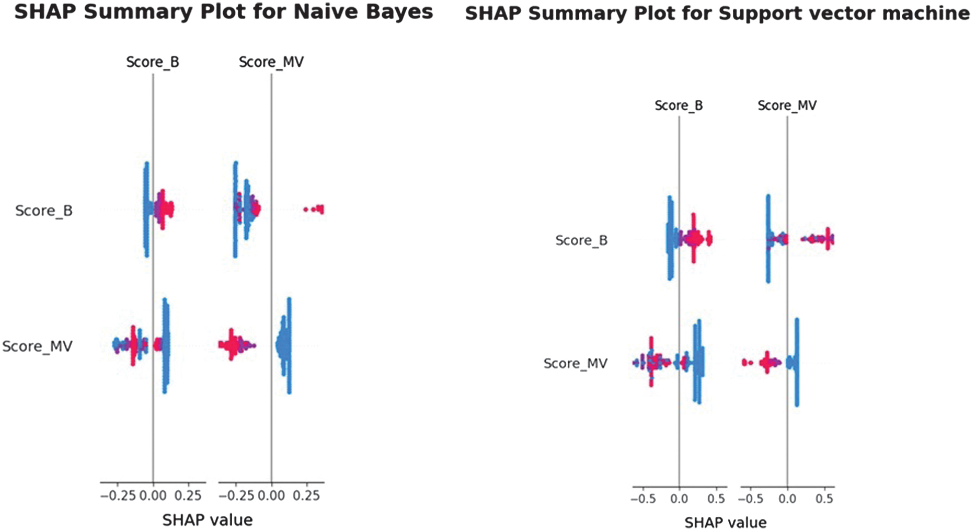Fig. 17. The SHAP summary diagram 1.

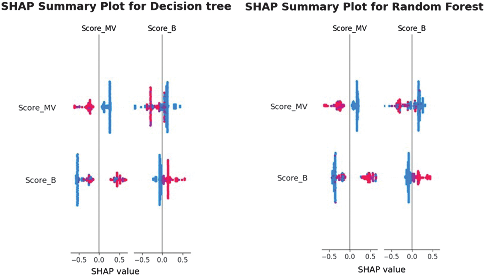Fig. 18. The SHAP summary diagram 2.

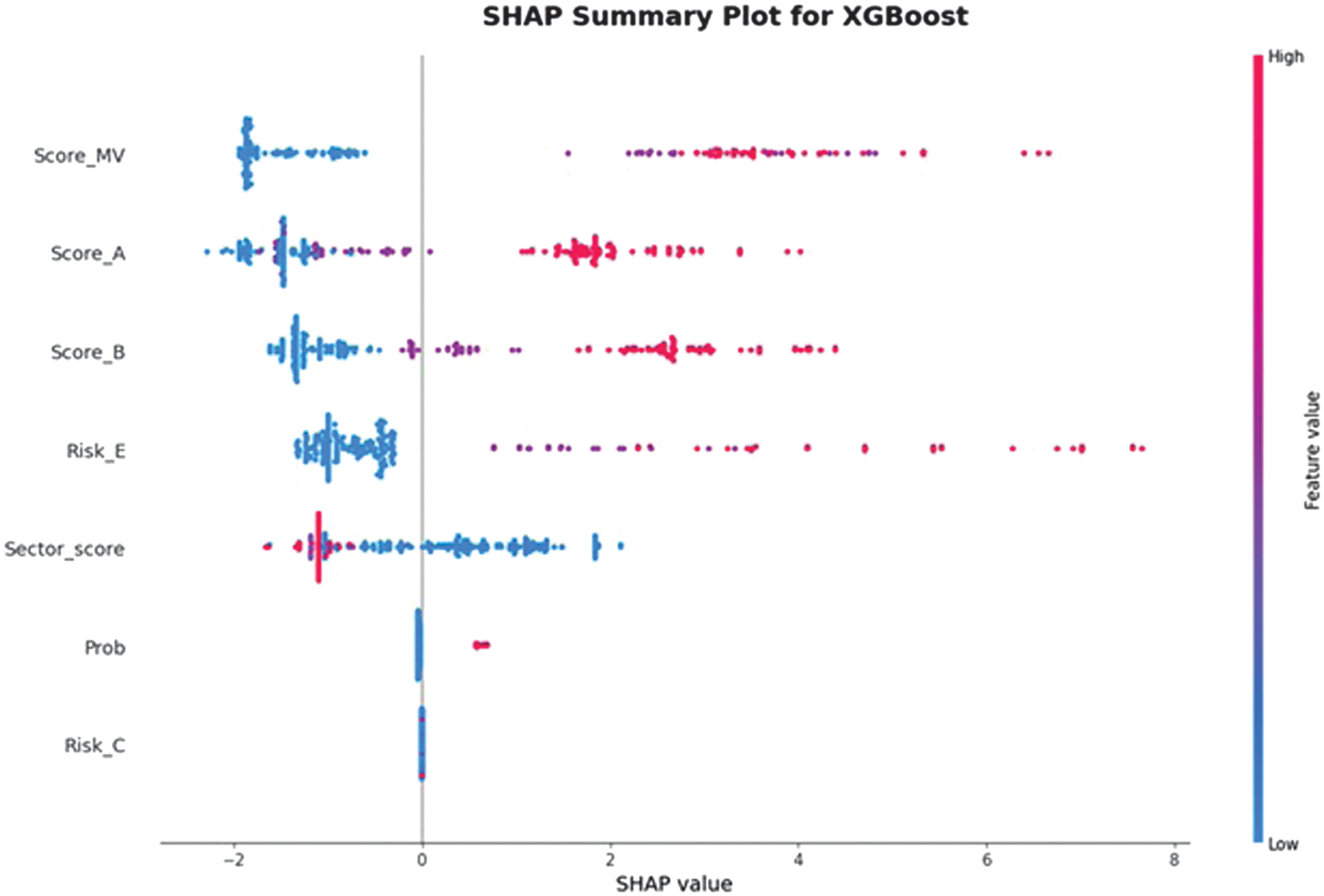Fig. 19. The SHAP summary diagram 3.

The SHAP analysis reveals consistent patterns in how the models utilize the available audit-related features. For the simpler models, such as NB, SVM, DT, and RF, the summary plots show that Score_MV and Score_B dominate the predictive behavior, with all remaining features contributing minimally or negligibly. This indicates that these models rely primarily on the binary scoring indicators to separate risky from non-risky units, reflecting their limited capacity to capture nonlinear interactions. In contrast, the XGBoost model exhibits a markedly richer and more distributed SHAP landscape: Score_MV, Score_A, Score_B, and Risk_E all have substantial impact on the model output, while Sector_score and Prob show moderate influence. This broader use of features suggests that XGBoost can incorporate more complex relationships in the dataset, resulting in different decision boundaries. The clear separation of positive and negative SHAP values across high- and low-risk feature levels further demonstrates that the model assigns risk in a directionally consistent and interpretable manner. Overall, the SHAP results confirm that, although baseline and linear models rely on a subset of strong predictors, the XGBoost model leverages a more comprehensive representation of the audit features, thereby enhancing both predictive accuracy and interpretability.

The dataset is classified using the described ML algorithms. The accuracy, precision, recall, and F1-score classification measures are used to evaluate the efficiency of developed models [29,30]. These measures are stated by Eq. (8)–(10):

accuracy = \frac{T P + T N}{T P + F P + T N + F N}

(8)

precision = \frac{T P}{T P + F P}

(9)

recall = \frac{T P}{T P + F N}

(10)

F 1_s c o r e = 2 \frac{precision \times r e c a l l}{precision + r e c a l l}

(11)

First, the data are divided into 75% for training and 25% for testing. Then, for ML models, the training data are split using cross-validation [31], creating folds for training and validating using different combinations of these parts (Fig. 20). Then the trained model is applied to the testing part. The classification results with the standard deviations of the K-fold cross-validation ML models on the training and testing parts with the Chi-square feature selection technique are shown in Tables IX and X. The additional experiments of classification of features chosen by the Mutual Information feature selection technique are conducted. The results are shown in Tables XI and XII.

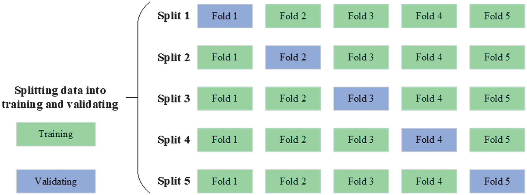Fig. 20. K-fold cross-validation [31].

Table IX. Classification results on the training part with the standard deviation using the Chi-square feature selection technique

Classifier	NB	SVM	DT	RF	XGBoost
Accuracy	0.849 ± 0.030	0.959 ± 0.015	0.957 ± 0.009	0.964 ± 0.009	0.956 ± 0.007
Precision	0.787 ± 0.028	0.965 ± 0.024	0.968 ± 0.016	0.983 ± 0.017	0.968 ± 0.016
Recall	0.953 ± 0.048	0.951 ± 0.017	0.945 ± 0.020	0.945 ± 0.023	0.942 ± 0.018
F1-score	0.862 ± 0.034	0.958 ± 0.017	0.956 ± 0.011	0.963 ± 0.011	0.955 ± 0.009

Table X. Classification results on the testing part using the Chi-square feature selection technique

Classifier	NB	SVM	DT	RF	XGBoost
Accuracy	0.846	0.949	0.957	0.949	0.944
Precision	0.785	0.942	0.958	0.921	0.934
Recall	0.958	0.958	0.958	0.983	0.958
F1-score	0.863	0.950	0.958	0.951	0.946

Table XI. Classification results on the training part, with the standard deviation using the Mutual Information feature selection technique

Classifier	NB	SVM	DT	RF	XGBoost
Accuracy	0.740 ± 0.157	0.906 ± 0.016	0.987 ± 0.009	0.989 ± 0.006	0.990 ± 0.009
Precision	0.799 ± 0.197	0.958 ± 0.034	0.983 ± 0.014	0.991 ± 0.007	0.989 ± 0.011
Recall	0.726 ± 0.050	0.848 ± 0.019	0.991 ± 0.007	0.986 ± 0.009	0.991 ± 0.007
F1-score	0.748 ± 0.114	0.899 ± 0.021	0.987 ± 0.009	0.989 ± 0.006	0.990 ± 0.009

Table XII. Classification results on the testing part with the Mutual Information feature selection technique

Classifier	NB	SVM	DT	RF	XGBoost
Accuracy	0.799	0.927	0.962	0.970	0.966
Precision	0.851	0.963	0.936	0.959	0.944
Recall	0.729	0.890	0.992	0.983	0.992
F1-score	0.785	0.925	0.963	0.971	0.967

The comparison of classification results using Chi-square and Mutual Information feature selection techniques shows noticeable quantitative differences across models. Using the Chi-square method, the training accuracy ranges from 0.849 for NB to 0.964 for RF, with RF and XGBoost achieving the highest F1-scores of 0.963 and 0.955, respectively. On the testing set, Chi-square maintains stable performance, with DT achieving an accuracy of 0.957 and an F1-score of 0.958, while RF achieves 0.949 accuracy and 0.951 F1-score, indicating good generalization and low performance degradation between the training and testing phases. In contrast, the Mutual Information feature selection technique results in significantly higher training performance for tree-based models. On the training data, RF and XGBoost achieve accuracy scores of 0.989 and 0.990, respectively, and F1-scores of 0.989 and 0.990, outperforming their Chi-square by approximately 2.5–3.5%. However, NB with Mutual Information shows lower and less stable performance, with training accuracy of 0.740 ± 0.157 and F1-score of 0.748 ± 0.114. On the testing set, Mutual Information-based selection outperforms Chi-square for advanced classifiers: RF achieves an accuracy score of 0.970 and an F1-score of 0.971; XGBoost achieves an accuracy of 0.966 and an F1-score of 0.967; and DT achieves an accuracy of 0.962 and an F1-score of 0.963, exceeding the Chi-square results. Overall, Mutual Information provides superior predictive performance for DT, RF, and XGBoost on both training and testing datasets, while Chi-square offers more balanced and stable results, particularly for simpler models such as NB and SVM. Next, the training and average inference time of ML models are evaluated. For brevity, the results for Chi-square feature selection are shown in Table XIII.

Table XIII. Training time and average inference time per sample for the Chi-square

Type of time (seconds)	NB	SVM	DT	RF	XGBoost
Training time	0.0018	0.0122	0.0037	0.0146	0.0770
Average inference time	0.0057	0.0065	0.0069	0.0089	0.0107

Table XIII presents the computational efficiency of the evaluated ML models for Chi-square in terms of training time and average inference time per sample. The results indicate clear differences in computational cost across algorithms. NB demonstrates the lowest training time (0.0018 s) and the fastest inference latency (0.0057 s), reflecting its simple probabilistic structure and suitability for large-scale, real-time audit screening. DT also exhibits low computational overhead, with a short training time (0.0037 s) and efficient inference (0.0069 s), making it a practical option when interpretability and speed are required. More complex ensemble models incur higher computational costs. RF and XGBoost show increased training times (0.0146 s and 0.0770 s, respectively) due to the construction of multiple trees and boosting iterations. However, their inference times remain within milliseconds per sample, indicating that their deployment remains feasible for offline or batch-based audit analysis. SVM has an intermediate position, with moderate training and inference times compared to simpler classifiers. Overall, the results demonstrate a trade-off between predictive performance and computational efficiency. While ensemble models achieve superior classification accuracy, simpler models such as NB and DT offer significant speed advantages. These findings support the practical feasibility of the proposed models and highlight that ensemble-based approaches can be deployed in organizational audit workflows without prohibitive computational cost, particularly when inference latency rather than training time is the primary operational concern. The calculated mean and deviation measures are supplemented with the t-test and p-value statistics. The paired t-test is a statistical hypothesis test used to determine whether the difference in mean performance between two models is statistically significant when they are evaluated under identical experimental conditions. In this study, the paired t-test compares the performance scores (accuracy, precision, recall, and F1-score) obtained by two classifiers on the same cross-validation folds. Because each fold is shared, the results are paired, removing variability introduced by data partitioning and providing a more reliable comparison. The t-test and p-value for an accuracy score of all ML models for Chi-square feature selection are shown in Table XIV.

Table XIV. The statistics scores for ML models for the Chi-square

Model A	Model B	t-Test	p-Value
NB	SVM	− 7.455	0.0017
NB	DT	− 6.687	0.0026
NB	RF	− 6.091	0.0037
NB	XGBoost	− 6.823	0.0024
SVM	NB	7.455	0.0017
SVM	DT	0.190	0.8589
SVM	RF	− 0.476	0.6587
SVM	XGBoost	0.376	0.7262
DT	NB	6.687	0.0026
DT	SVM	− 0.190	0.8589
DT	RF	− 2.135	0.0997
DT	XGBoost	1.000	0.3739
RF	NB	6.091	0.0037
RF	SVM	0.476	0.6587
RF	DT	2.135	0.0997
RF	XGBoost	2.205	0.0921
XGBoost	NB	6.823	0.0024
XGBoost	SVM	− 0.376	0.7262
XGBoost	DT	− 1.000	0.3739
XGBoost	RF	− 2.205	0.0921

The results indicate that SVM, DT, RF, and XGBoost models outperform NB (p-values < 0.01), demonstrating robust, statistically significant improvements over the baseline. In contrast, comparisons among SVM, DT, RF, and XGBoost yield p-values > 0.05, indicating that their accuracies are statistically comparable. These findings suggest that while replacing NB with more sophisticated classifiers leads to a clear and significant gain in accuracy, no single advanced model can be claimed to be superior to the others based on statistical evidence alone. The classification results for the DL models and the Chi-square feature selection technique are shown in Table XV, and the classification results with the Mutual Information feature selection technique are shown in Table XVI. The training and average inference time of DL models are shown in Table XVII.

Table XV. Classification results on the testing part with the Chi-square feature selection technique

Classifier	DNN	CNN	LSTM	CNN-LSTM	LSTM-GRU
Accuracy	0.949	0.838	0.880	0.850	0.880
Precision	0.934	0.845	0.941	0.888	0.941
Recall	0.966	0.831	0.814	0.805	0.814
F1-score	0.950	0.838	0.873	0.844	0.873

Table XVI. Classification results on the testing part with the Mutual Information feature selection technique

Classifier	DNN	CNN	LSTM	CNN-LSTM	LSTM-GRU
Accuracy	0.927	0.880	0.910	0.795	0.889
Precision	0.939	0.852	0.929	0.724	0.918
Recall	0.915	0.924	0.890	0.958	0.856
F1-score	0.927	0.886	0.909	0.825	0.886

Table XVII. Training time and average inference time per sample

Type of time (seconds)	DNN	CNN	LSTM	CNN-LSTM	LSTM-GRU
Training time	7.39	10.01	11.60	10.48	12.58
Average inference time	0.07	0.10	0.12	0.10	0.13

The DL results illustrate how the choice of feature selection technique influences model behavior and generalization. In Table XV, with the Chi-square feature selection, DNN achieves the best overall performance, with an accuracy of 0.949 and an F1-score of 0.950, supported by a high recall of 0.966, indicating strong sensitivity to risky entities. The LSTM and LSTM-GRU models show moderate, comparable performance, both achieving an accuracy of 0.880 and an F1-score of 0.873, while the CNN-LSTM achieves slightly lower values, with an accuracy of 0.850 and an F1-score of 0.844. CNN performs worst in this setting, with an accuracy of 0.842 and an F1-score of 0.848, suggesting that pure convolutional architectures are poorly suited to tabular audit data. When applying the Mutual Information feature selection in Table XVI, performance patterns change noticeably. While DNN experiences a decline in accuracy from 0.949 to 0.927 and in F1-score from 0.950 to 0.927, recurrent architectures benefit from the Mutual Information-selected features. LSTM improves to 0.910 in accuracy and 0.909 in F1-score, while CNN-LSTM increases recall from 0.805 to 0.958, indicating that Mutual Information emphasizes features strongly associated with the risk class. LSTM-GRU improves slightly to an accuracy of 0.889 and an F1-score of 0.886. Overall, Chi-square feature selection favors stable, well-balanced performance, particularly for DNNs, while Mutual Information enhances recall and class separability for recurrent and hybrid architectures. These results confirm that DL models respond differently to feature selection strategies and that no single method universally dominates.

Table XVII reports the training time and average inference time per sample for the evaluated DL models. Compared to classical ML approaches, all DL architectures exhibit substantially higher training times, reflecting their increased architectural complexity and iterative optimization procedures. DNN shows the lowest training cost among the deep models (7.39 s), followed closely by CNN (10.01 s) and CNN-LSTM (10.48 s). It indicates that shallow feed-forward and convolutional architectures converge relatively efficiently on the given dataset. Sequential and hybrid recurrent architectures incur higher computational overhead. LSTM and LSTM-GRU models exhibit the longest training times (11.60 s and 12.58 s, respectively), which is expected given their recurrent structure and gate-based memory mechanisms. Despite differences in training costs, the average inference time per sample remains relatively stable across all DL models, ranging from 0.10 s to 0.13 s. It suggests that while training complexity varies significantly, inference latency is less sensitive to architectural differences and remains feasible for offline audit risk assessment. Overall, these results highlight a clear trade-off between model complexity and computational efficiency. Although DL models offer expressive representational capacity, their increased training cost and marginal inference-time advantage limit their practical appeal for routine organizational audit deployment. Consequently, unless large-scale data or temporal dependencies justify their use, simpler ensemble-based models may provide a more computationally efficient and operationally practical solution.

The accuracy, loss, and confusion matrices plots [38,39] using Matplotlib and Seaborn libraries [40,41] are shown in Figs. 21–25. The histograms, AUC-ROCs, AUC-PRs, and calibration curves with Brier scores are shown in Figs. 26–29.

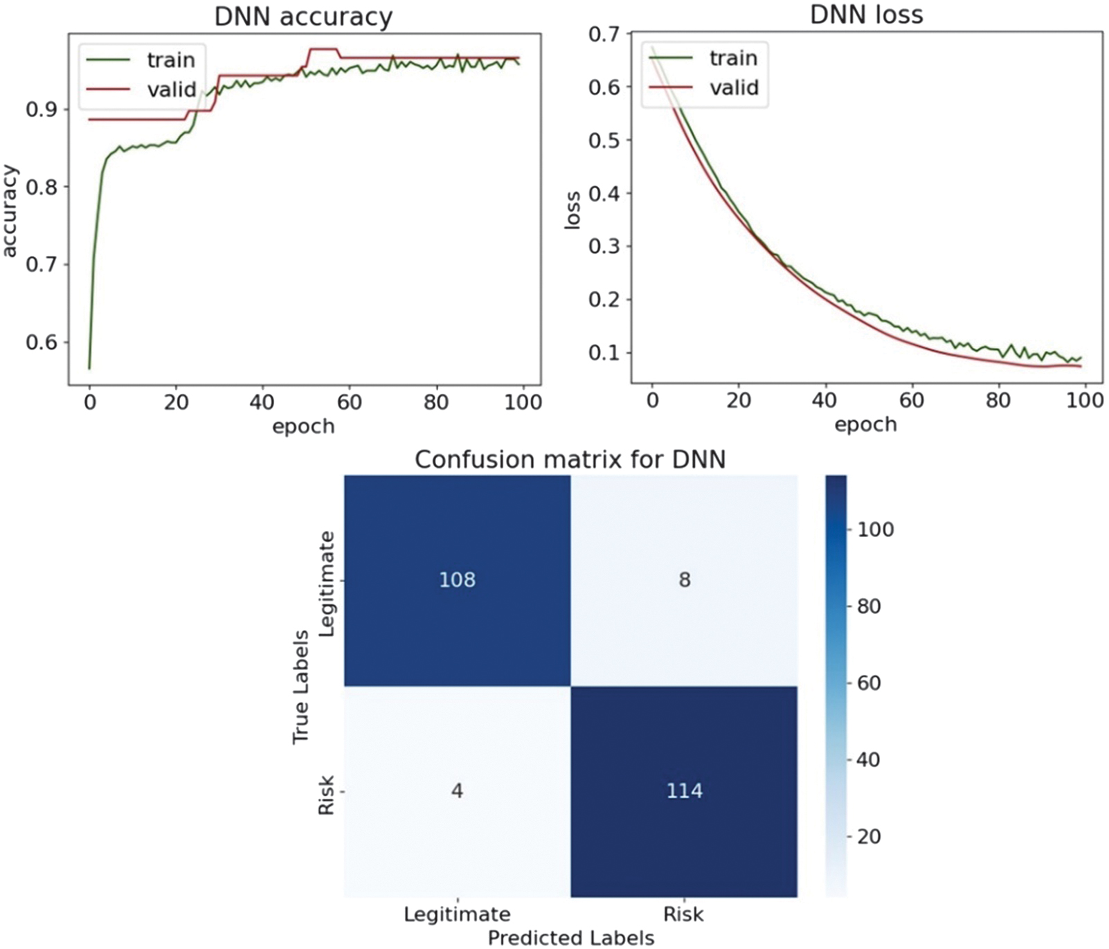Fig. 21. The classification plots of DNN.

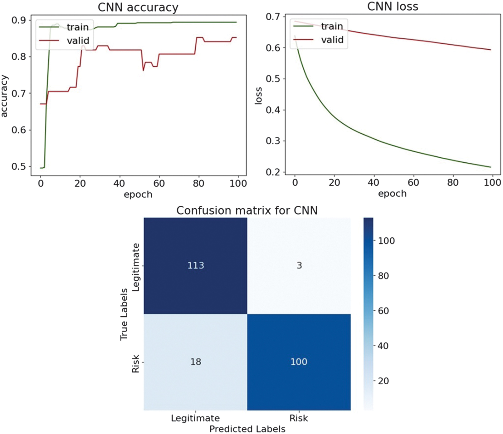Fig. 22. The classification plots of CNN.

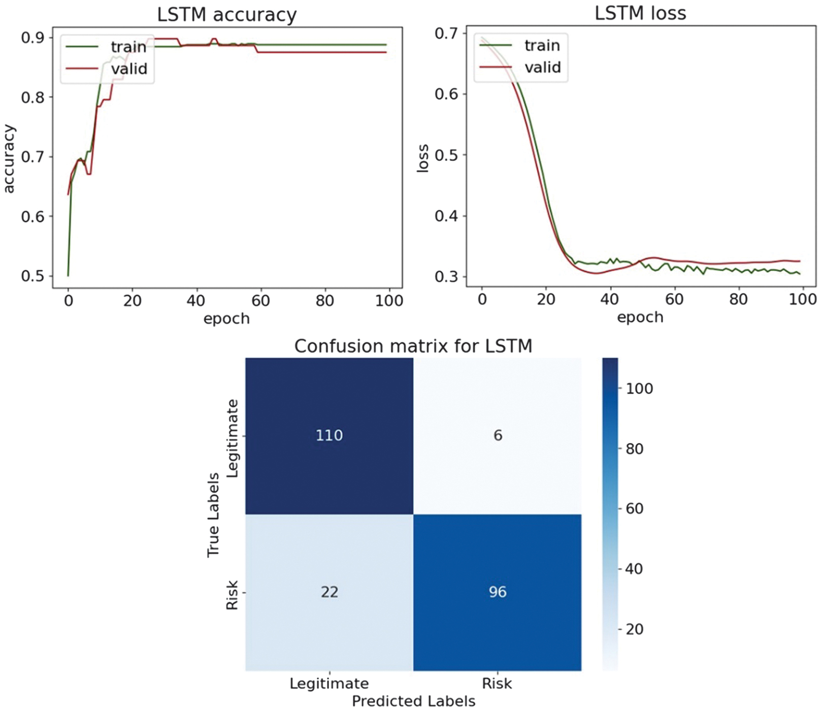Fig. 23. The classification plots of LSTM.

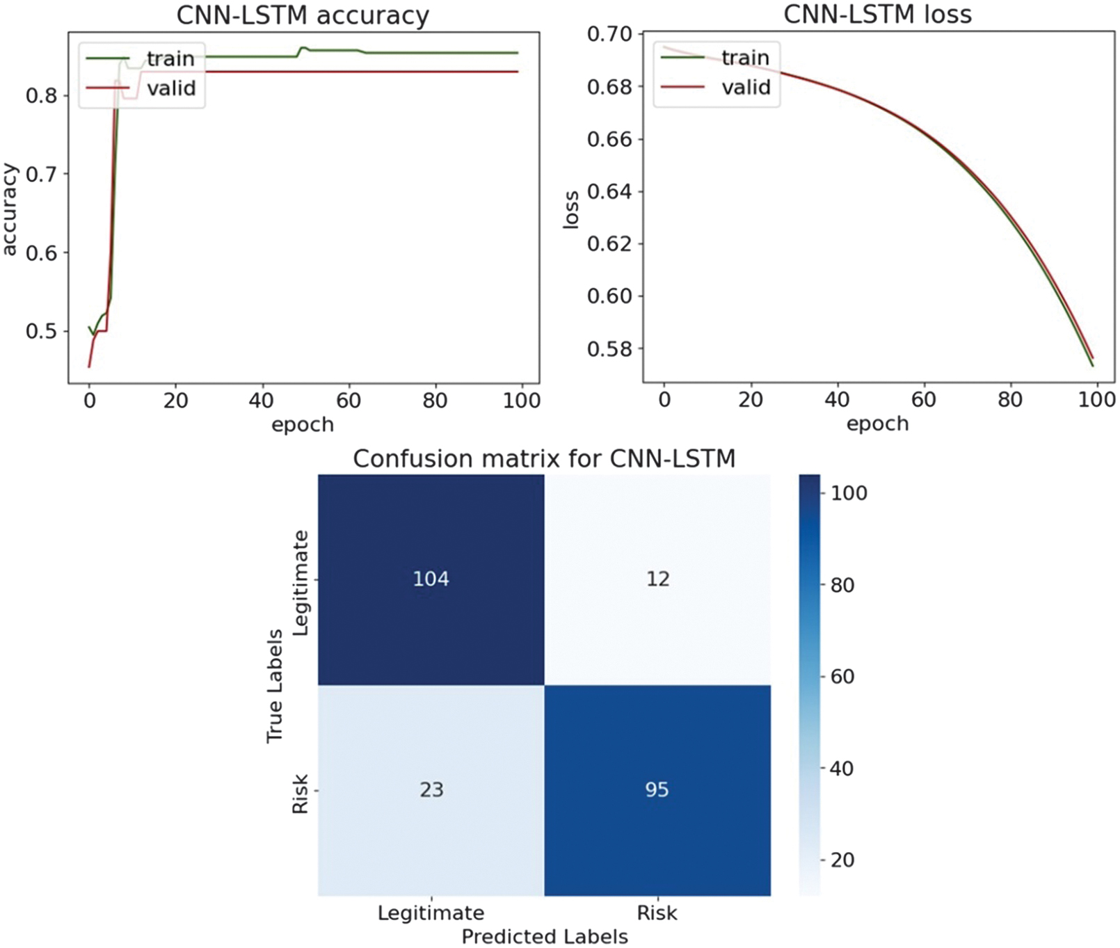Fig. 24. The classification plots of CNN-LSTM.

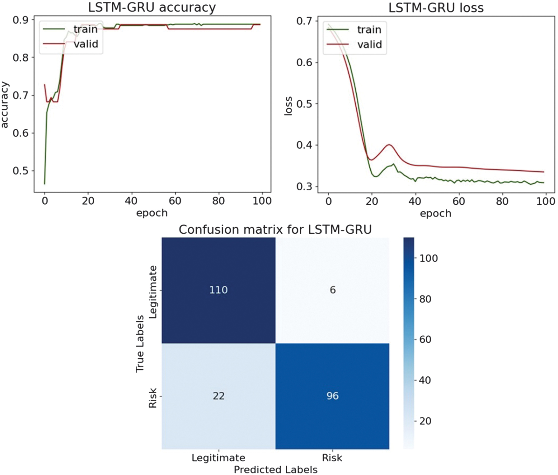Fig. 25. The classification plots of LSTM-GRU.

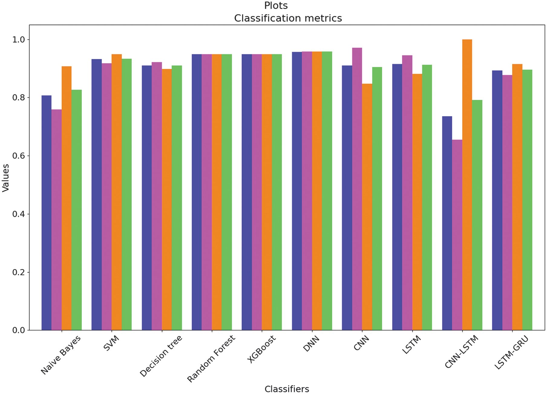Fig. 26. Classification histograms for each algorithm with accuracy, precision, recall, and F1-score metrics.

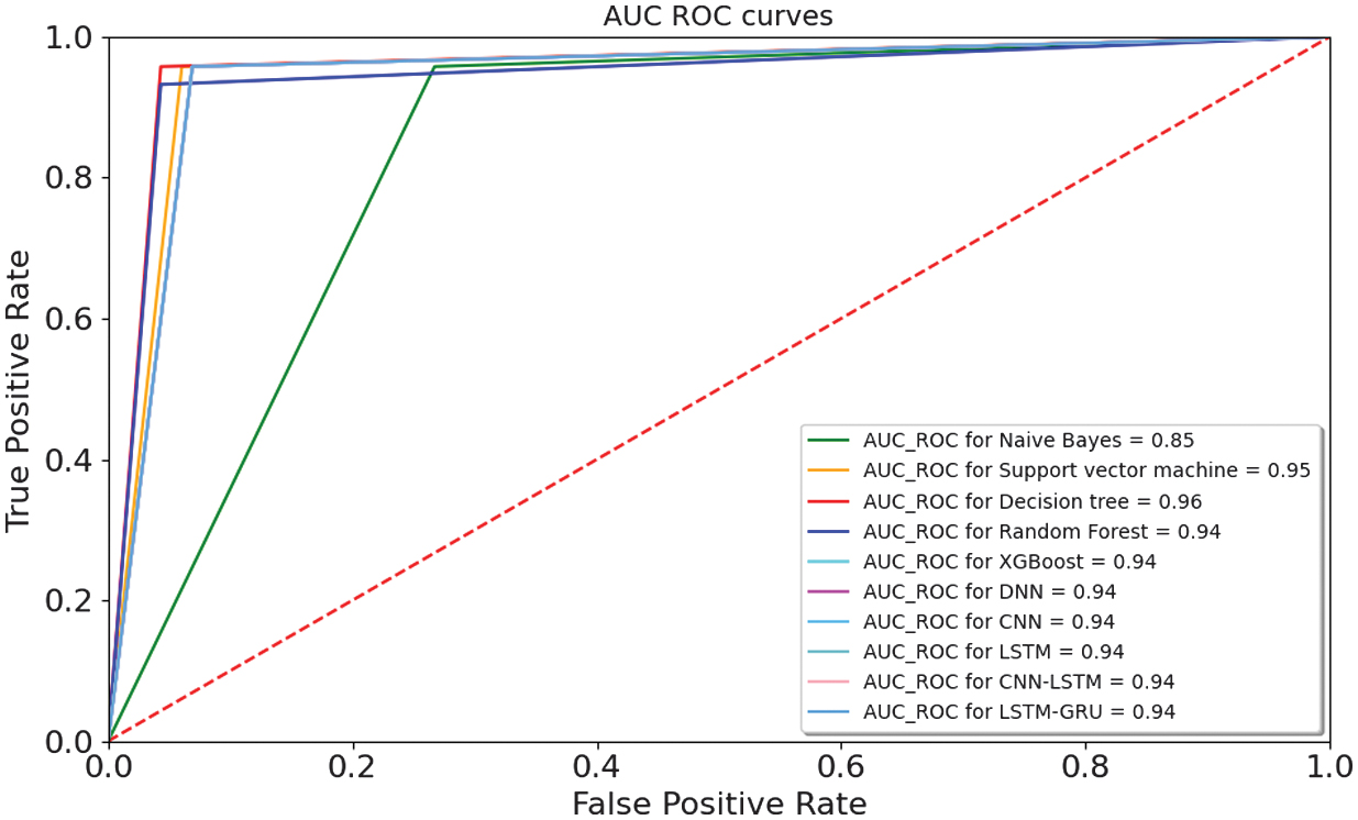Fig. 27. AUC–ROCs for classification algorithms.

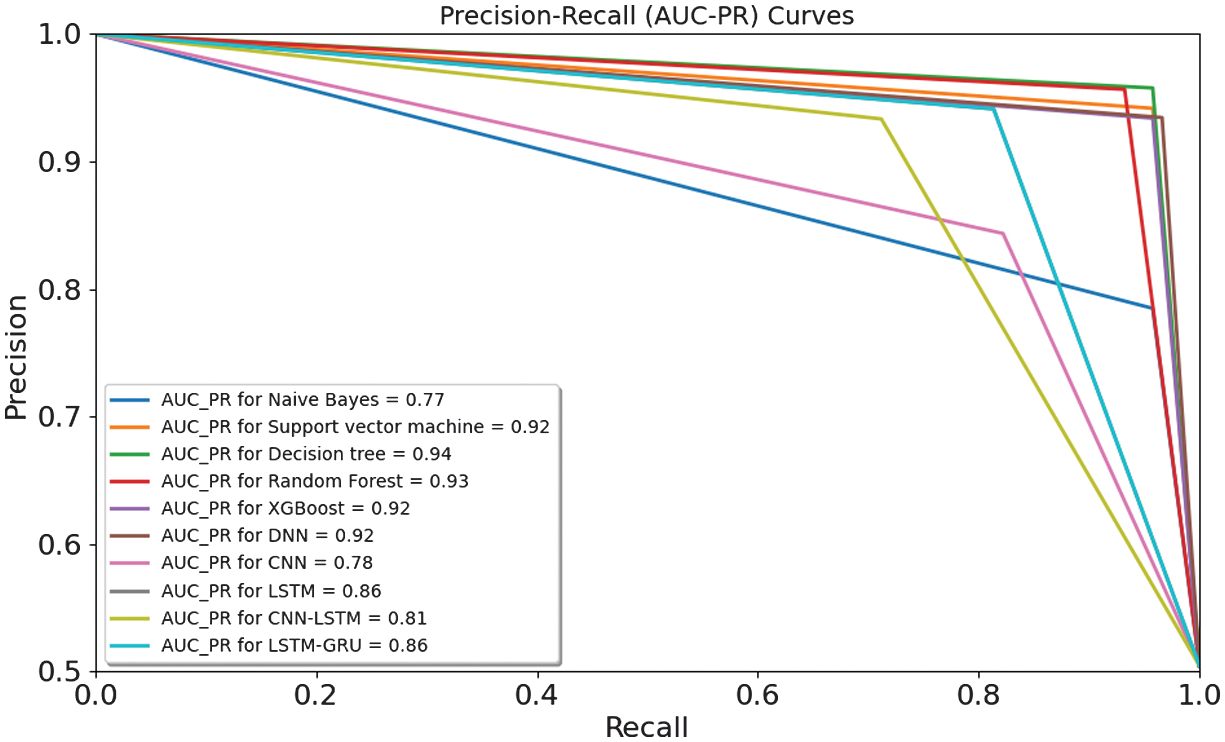Fig. 28. AUC–PRs for classification algorithms.

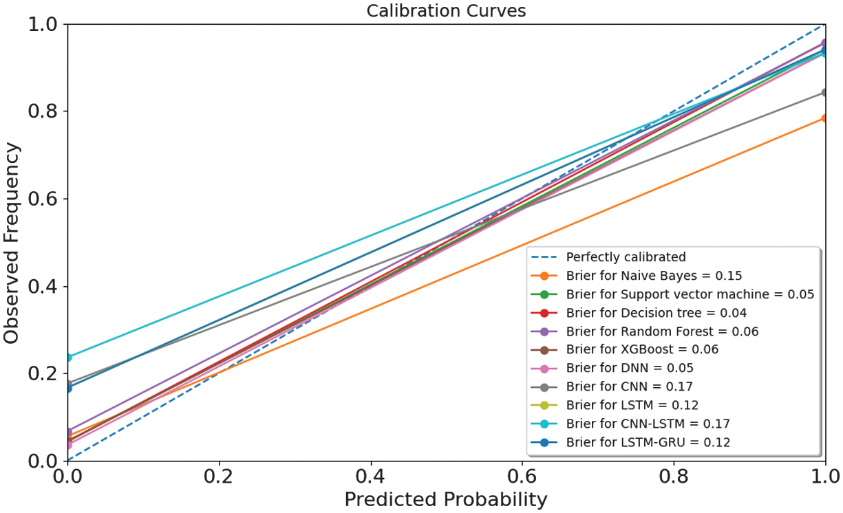Fig. 29. The calibration curves with Brier scores.

The evaluation of results with classification plots, AUC-ROCs, AUC-PRs, and calibration curves provides a comprehensive view of both the discriminative power and probability reliability of the proposed models. Most ensemble and DL models achieve very high AUC-ROC values of 0.94–0.95, indicating strong global ranking ability between risky and non-risky organizations. However, in an imbalanced audit context, AUC-PR is a more informative metric, as it directly reflects the trade-off between precision and recall for the minority class. The AUC-PR results demonstrate that XGBoost and DNN models achieve the strongest risky-class detection performance, confirming that their high accuracy is not driven solely by the majority class. Beyond ranking, calibration curves and Brier scores reveal how well predicted probabilities match the true empirical risk frequencies. The low Brier scores of 0.04–0.06 indicate that the predicted audit risk probabilities are well calibrated and suitable for probability-based decision-making. From an operational standpoint, false negatives incur substantially higher costs than false positives, as they may lead to undetected fraud, financial losses, and regulatory violations, whereas false positives mainly increase audit workload. Consequently, decision thresholds are not fixed at 0.5 but are selected using cost-sensitive criteria, favoring lower thresholds to maximize recall of risky entities while keeping the additional audit burden at an acceptable level. This thresholding strategy, supported by the AUC-PR and calibration analysis, ensures that the models are not only statistically accurate but also aligned with real-world audit risk management objectives.

Overall, the experiments show that ensemble learning methods and DL architectures with memory components, such as LSTM-GRU, are particularly effective for achieving high classification accuracy and balanced predictive performance.

For practical adoption in organizational auditing, the proposed intelligent risk assessment framework is designed to function as a decision-support tool rather than a fully automated replacement for auditors. In a typical workflow, the model would be integrated into the early planning and risk assessment phase of an audit. Organizational data are processed through the trained classification model to generate risk scores and binary risk labels for audited entities. These outputs enable auditors to prioritize entities, processes, or documents that require deeper examination, thereby optimizing the allocation of audit resources. User interaction with the system is assumed at multiple stages. Auditors are provided with model predictions and SHAP-based explanations that highlight the most influential risk indicators contributing to each high-risk classification. Consistently high SHAP contributions for governance-related or operational risk features may prompt targeted control testing or interviews. This interpretation aligns with risk-based auditing principles, where explainability supports transparency and traceability of audit judgments. Crucially, the framework incorporates override and validation mechanisms to preserve professional judgment. Auditors may override model predictions based on domain knowledge, contextual information, or evidence not captured in the data. Such overrides can be logged for documentation and post-audit review, ensuring accountability and compliance with audit standards. This approach ensures that automated assessments augment rather than constrain auditor expertise. The proposed decision protocol follows a structured sequence: automated risk scoring and classification, explainability-driven review using SHAP outputs, auditor validation or override based on professional assessment, and final audit decisions supported by documented evidence. By combining predictive analytics with transparent explanations and human oversight, the framework aligns with established audit and compliance practices and supports responsible deployment of AI in organizational auditing.

V.CONCLUSION

This research highlighted the effectiveness of integrating ML and DL models into organizational auditing to identify and evaluate systematic risk. The experimental analysis was conducted on a dataset of 773 organizational units using a multi-stage pipeline that included scaling, feature selection, Correlation analysis, SHAP analysis, and classification with ML and DL models. The sensitivity analysis was performed by reducing the original 26 features to the top-10 and top-14 ranked variables and then to a compact subset of 7 features after removing highly correlated ones. The classification results with Chi-square feature selection closely matched cross-validated training performance, achieving 0.956–0.964 in accuracy for XGBoost and RF models. In the NN scenario, DNN achieved the best results, with an accuracy of 0.949 and an F1 of 0.950, but LSTM, CNN-LSTM, and LSTM-GRU showed moderate performance, with accuracy scores of 0.850–0.880 and F1-scores of 0.844–0.873. The Mutual Information feature selection increased predictive separability, with DT and RF achieving accuracy scores of 0.987-0.990, respectively, and XGBoost achieving 0.990. In DL experiments, performance shifted toward higher sensitivity to risky entities: LSTM improved to 0.910, CNN-LSTM achieved a recall of 0.958, and LSTM-GRU reached an accuracy of 0.889. Overall, the Chi-square showed balanced and stable DL performance, whereas Mutual Information enhanced recall and class separability for recurrent and hybrid models. Generally, the significance of this research lies in its direct applicability to real-world organizational auditing and risk management. Overall, the proposed framework demonstrated how ML and DL models could be systematically integrated into audit workflows to support early risk identification, audit prioritization, and efficient allocation of audit resources. In future work, it is planned to expand the audit dataset and integrate additional ML and DL models.

The Identification of Risk Organizations with Machine Learning and Deep Learning Models

I.INTRODUCTION

II.LITERATURE REVIEW

III.METHODOLOGY

IV.RESULTS AND DISCUSSION

V.CONCLUSION

DATA AVAILABILITY

FUNDING STATEMENT

ACKNOWLEDGMENTS

CONFLICT OF INTEREST STATEMENT

REFERENCES