JAIT

I.INTRODUCTION

In unstructured and non-convex environments such as dense forests and urban ruins, collaborative navigation for multi-unmanned aerial vehicle (UAV) systems represents a pivotal challenge in contemporary robotics [1]. The fundamental objective of formation control in such scenarios involves a coupled dual task: maintaining geometric rigidity of the communication topology through distributed collaboration and ensuring the real-time generation of collision-free safe trajectories [2–4]. Fig. 1 shows the multi-UAV formation overview generally. The formation has to operate in a complex environment with static obstacles, dynamic obstacles, and stable data links.

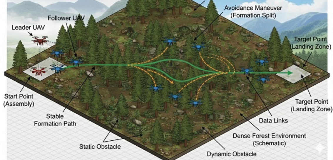Fig. 1. Multi-UAV formation flight graph.

Algebraic graph theory and second-order consensus protocols have been widely used to ensure the asymptotic synchronization of multi-agent systems. To endow these systems with reactive obstacle avoidance capabilities, the artificial potential field (APF) method is frequently integrated into control laws due to its computational efficiency and explicit physical interpretability. However, traditional APF algorithms suffer from inherent topological defects [5]. Their static parameter configurations lack the adaptability required to cope with highly dynamic spatial constraints. More critically, in non-convex obstacle spaces such as U-shaped traps or symmetric obstacles, inevitably trapping the UAV in a deep local minimum leads to severe motion deadlock or persistent trajectory oscillation [6]. Traditional remedial measures, such as introducing virtual targets or constructing orthogonal vortex fields, are mostly rule-based and geometrically rigid. These geometric reconstruction methods heavily rely on prior knowledge of obstacle distribution, making it difficult to generalize in dynamically changing unstructured environments. They merely alleviate the appearance of local minima but fail to adaptively address the essence of underlying collinear force conflicts [7].

In recent years, deep reinforcement learning (DRL) has demonstrated remarkable performance in continuous control tasks, providing model-free adaptability to complex environments [8,9]. Despite its empirical success, the deployment of pure “End-to-End” DRL in safety-critical flight control remains highly constrained. The End-to-End framework directly maps high-dimensional state observations to low-level motor commands, introducing significant semantic opacity and structural fragility. This “black box” paradigm makes rigorous stability analysis based on Lyapunov mathematically intractable, leading to a high risk of catastrophic failures when the system encounters out-of-distribution (OOD) states [10].

The theory of multi-UAV formation control primarily relies on two architectures: centralized and distributed [11]. Inspired by the collective behavior of biological groups such as bee colonies, flocks of geese, and schools of fish in nature, UAV formation control technology aims to achieve macro-level formation maintenance and adaptation through collaboration among individuals [12]. However, current multi-UAV collaborative tasks primarily focus on task planning and allocation at the upper level, with less attention paid to the formation flight of the underlying UAV formation and the coordination of position and velocity among internal members [13,14].

To integrate the cognitive adaptability of DRL with the deterministic safety of classical control theory, this paper proposes a hierarchical meta-control architecture. Based on a leader–follower augmented graph topology, the proposed framework strategically allocates structural maintenance tasks to followers through distributed consensus control laws. For the leader, a twin delay deep deterministic policy gradient (TD3) agent is introduced, which is not intended to replace the physical controller but to modulate it. Specifically, the TD3 agent dynamically optimizes the APF gain in real time and crucially outputs a continuous rotational yaw angle. This learnable mechanism actively reconstructs the topological structure of the repulsive force field, fundamentally breaking the mechanical equilibrium of local minima by generating non-collinear tangential forces.

II.PROBLEM FORMULATION AND SYSTEM MODELING

A.PROBLEM FORMULATION

The multi-UAV formation flight mission refers to the process of dispatching multiple UAVs to take off from the starting point, traverse obstacle-filled areas, and collaboratively fly to the target point. The UAV formation needs to fly to the target point while maintaining its formation. When there are obstacles in the path map, the UAV formation needs to bypass static obstacles and urgently avoid corresponding dynamic obstacles [15]. During the obstacle avoidance process, the UAV formation needs to make corresponding maneuvers, appropriately reduce the need to maintain the UAV formation, and prioritize obstacle avoidance, and after completing obstacle avoidance, the UAV formation needs to respond quickly and restore the desired formation in a timely manner [16].

Multi-UAV formation flight in unstructured non-convex environments faces prominent technical challenges rooted in the inherent defects of traditional APF algorithms [17,18]. Static parameter configurations of the algorithm lack adaptability to dynamic spatial constraints, easily leading to UAV entrapment in local minima and subsequent motion deadlock or trajectory oscillation [19]. Pure end-to-end DRL methods suffer from semantic opacity and structural fragility, making rigorous stability analysis difficult and posing high safety risks in safety-critical flight control scenarios. Conventional remedial measures for local minima are mostly rule-based with poor generalization, failing to adaptively resolve the underlying collinear force conflict issues. Meanwhile, the lack of effective integration between reinforcement learning and consensus protocols results in difficulty balancing the dual demands of formation geometric rigidity maintenance and real-time agile obstacle avoidance in complex environments, and the nonautonomous closed-loop system with time-varying parameters lacks theoretical support for stability guarantees [20].

B.SYSTEM MODELING

The research focus of this paper lies in multi-UAV formation flight in complex environments. Specifically, this paper emphasizes the formation maintenance and obstacle avoidance issues during UAV formation flight, thus simplifying the motion characteristics of UAVs to some extent. This paper adopts a constrained kinematic model to model UAVs as point mass models in a two-dimensional scenario [21]. The model is constructed based on the pygame simulation environment, accurately describing the motion behavior of UAVs in a two-dimensional inertial coordinate system through discrete time difference equations.

1).DEFINITION OF STATE SPACE

Assuming that the formation system is composed of $N$ UAVs, the state vector $x_{i} (t)$ of the i-th UAV ( $i = 1, \dots, N$ ) at time $t$ is defined as:

x_{i} (t) = {[x_{i} (t), y_{i} (t), θ_{i} (t), v_{i} (t)]}^{T}

(1)

where

(x_{i}, y_{i})

represents the position coordinates of the UAV in the two-dimensional inertial Cartesian coordinate system,

θ_{i} (t) \in [0, 2 π)

represents the heading angle of the UAV, defined as the angle between the velocity vector and the positive direction of the x-axis, with the counterclockwise direction being considered positive, and

v_{i} (t)

represents the magnitude of the linear velocity of the UAV.

The control input vector for the UAV is defined as $u_{i} (t)$ including linear acceleration commands and angular velocity commands:

u_{i} (t) = {[a_{i}^{c} (t), ω_{i}^{c} (t)]}^{T}

(2)

where

a_{i}^{c}

is used to control the rate of change of speed and

ω_{i}^{c}

is used to control the rate of change of heading angle.

2).DISCRETE TIME KINEMATIC EQUATION

Given that the simulation environment updates states based on discrete time steps, let the system sampling time interval be $Δ t$ . At time $k$ , the state changes of the i-th UAV are first updated for speed and heading, and then the position is updated based on the updated speed. The specific dynamic equation modeling is as follows.

The linear velocity of the UAV is controlled solely by the longitudinal acceleration command, and a sensitivity coefficient $K_{a}$ is introduced to simulate the response characteristics of the underlying dynamic system. The linear velocity update equation is given as:

v_{i} (k + 1) = Clip (v_{i} (k) + K_{a} \cdot a_{i}^{c} (k), v_{\min}, v_{\max})

(3)

where

K_{a}

represents the acceleration sensitivity coefficient and the function

Clip (v_{\min}, v_{\max})

represents the speed saturation constraint, ensuring that the flight speed is always maintained within the allowable range.

The steering motion of the UAV is driven by angular velocity commands, and its heading angle discrete update formula is given as:

Ω_{i} (k) = Clip (K_{ω} \cdot ω_{i}^{c} (k), - Ω_{\max}, Ω_{\max})

(4)

θ_{i} (k + 1) = Mod (θ_{i} (k) + Ω_{i} (k) \cdot Δ t, 2 π)

(5)

where

K_{ω}

represents the angular velocity sensitivity coefficient,

Ω_{\max}

represents the maximum turning rate of the UAV, and

Mod (\cdot, 2 π)

is used to normalize the angle to the interval [0,2π), ensuring the continuity of the heading angle.

The update of the UAV’s position is based on the updated linear velocity $v_{i} (k + 1)$ and heading angle $θ_{i} (k + 1)$ . The position update of the UAV within a two-dimensional plane satisfies the following kinematic relationship:

{\begin{cases} x_{i} (k + 1) = x_{i} (k) + v_{i} (k + 1) \cos (θ_{i} (k + 1)) \cdot Δ t \\ y_{i} (k + 1) = y_{i} (k) - v_{i} (k + 1) \sin (θ_{i} (k + 1)) \cdot Δ t \end{cases}

(6)

The y-axis update term employs subtraction to adapt to the coordinate system definition of the simulation platform, with the downward y-axis being positive. In theoretical analysis, coordinate transformation can be equivalent to the standard Cartesian coordinate system.

3).PHYSICAL CONSTRAINTS AND NONHOLONOMIC CONSTRAINTS

Nonholonomic constraints: This model cannot achieve instantaneous lateral movement, and its motion must satisfy the condition of pure rolling without slipping, meaning that the instantaneous velocity direction of the UAV must be consistent with the direction of its nose:

{\dot{y}}_{i} (t) \cos θ_{i} (t) - {\dot{x}}_{i} (t) \sin θ_{i} (t) = 0

(7)

Maneuverability constraints: Based on the aerodynamic characteristics and actuator limitations of the aircraft, the state variables must satisfy the following hard boundaries:

{\begin{cases} v_{i} (t) \in [v_{\min}, v_{\max}] \\ | {\dot{θ}}_{i} (t) | \leq Ω_{\max} \end{cases}

(8)

where

v_{\min} > 0

indicates that the UAV cannot hover during flight. When the UAV reaches the target point or encounters a deadlock area, it must adopt hovering or other maneuvering strategies.

Environmental boundary constraints: The flight mission area is assumed to be a rectangular closed set $D = [x_{\min}, x_{\max}] \times [y_{\min}, y_{\max}]$ . During the simulation process, if the position state of the UAV exceeds this area, the system will forcibly perform clipping on its coordinates to simulate the blocking effect of physical fences:

p_{i} (k + 1) = Clip (p_{i} (k + 1), p_{\min}, p_{\max})

(9)

In addition to the limitations and realizations of UAV maneuverability, UAVs are also constrained by their detection range. Due to the performance limitations of onboard sensors, UAVs are unable to obtain comprehensive environmental information. The perception and detection radius of the i-th UAV is defined as $R_{sense}$ , and at time $t$ , the observation space $Z_{i} (t)$ of UAV $i$ is defined as a circular area centered at its own position $p_{i} (t)$ with a radius of $R_{sense}$ :

Z_{i} (t) = {q \in D | ‖ q - p_{i} (t) ‖ \leq R_{s e n s e}}

(10)

In addition, a UAV intelligent agent can only obtain the position and velocity information of obstacles located within $Z_{i} (t)$ .

C.STATE SPACE CONSTRUCTION

1).STATE SPACE

If a UAV formation system contains $N$ UAVs, we define the state vector $x_{i} (t)$ of i-th ( $i = 1, \dots, N$ ) UAV as [22]:

x_{i} (t) = {[x_{i} (t), y_{i} (t), θ_{i} (t), v_{i} (t)]}^{T}

(11)

where

(x_{i}, y_{i})

denotes the position coordinates of the UAV in a two-dimensional inertial Cartesian coordinate system,

θ_{i} (t) \in [0, 2 π)

denotes the heading angle of UAV, defined as the angle between the velocity

N

vector and the positive direction of the x-axis, with the counterclockwise direction being considered positive, and

v_{i} (t)

denotes the linear velocity of UAV.

The control input $i = 1, \dots, N$ vector for the UAV is defined as $u_{i} (t)$ , comprising linear acceleration commands and angular velocity commands:

u_{i} (t) = {[a_{i}^{c} (t), ω_{i}^{c} (t)]}^{T}

(12)

where

a_{i}^{c}

is used to control the rate of change of speed and

ω_{i}^{c}

is used to control the rate of change of heading

x_{i} (t)

angle.

To overcome the issues of slow convergence and poor physical interpretability caused by “black box” inputs in traditional end-to-end control [23], this paper designs an information-enhanced state space. The state vector $s_{t} \in R^{21}$ not only contains the kinematic information of the UAV but also explicitly embeds the force vector characteristics of the current physical field, reducing the difficulty for neural networks to understand the physical laws of the environment:

s_{t} = [s_{kin}, s_{nav}, s_{risk}, s_{force}, s_{meta}]

(13)

where kinematic characteristics

s_{kin} \in R^{4}

include the normalized position

(x, y)

of the UAV in the inertial frame and the linear velocity

(v_{x}, v_{y})

in the body frame.

The navigation feature $s_{risk} \in R^{5}$ refers to the relative normalized coordinates $({\tilde{g}}_{x}, {\tilde{g}}_{y})$ of the target point, guiding the agent to perceive the progress of the task.

The risk perception feature $s_{risk} \in R^{5}$ is represented by the relative position vector $(Δ x_{obs}, Δ y_{obs})$ and normalized distance $d_{\min}$ of the nearest obstacle.

The dual-threshold zone indicator $I_{outer}, I_{inner} \in {0, 1}$ comprises two Boolean variables, each indicating whether the UAV has entered the “warning zone” or “danger zone”. This discrete feature assists the network in swiftly recognizing the current risk level.

The mechanical perception feature $s_{force} \in R^{4}$ is composed of the normalized attractive force vector ${\tilde{F}}_{att}$ and the repulsive force vector ${\tilde{F}}_{rep}$ under current parameters. The calculation results of the APF are fed back to the network to obtain the suggested direction for the current physical model of the agent.

Meta-parameter feature $s_{meta} \in R^{6}$ comprises the action parameters output $k_{att}, k_{rep}$ at the previous moment and the repulsive force direction vector. This ensures the continuity of the strategy in the time dimension, facilitating the critic network to evaluate the long-term value of parameter adjustments.

2).COMPOSITE PARAMETER ACTION SPACE

To endow UAVs with multidimensional obstacle avoidance capabilities, enabling them to adjust both the strength and direction of the force field, the action space $a_{t} \in {[- 1, 1]}^{4}$ is defined as the normalized correction of potential field parameters:

a_{t} = [{\tilde{a}}_{1}, {\tilde{a}}_{2}, {\tilde{a}}_{3}, {\tilde{a}}_{4}]

(14)

k_{att} = map ({\tilde{a}}_{1}, [k_{att}^{\min}, k_{att}^{\max}])

(15)

k_{rep} = map ({\tilde{a}}_{2}, [k_{rep}^{\min}, k_{rep}^{\max}])

(16)

where the

m i n / m a x

superscript denotes the upper and lower bounds of the physical gain parameter. The gain adjustment action (

{\tilde{a}}_{1}, {\tilde{a}}_{2}

) converts the action value into a physical gain coefficient through linear mapping. The directional deflection action (

{\tilde{a}}_{3}, {\tilde{a}}_{4}

) does not directly correspond to an angle but rather serves as a two-dimensional deflection vector

δ_{dir} = [{\tilde{a}}_{3}, {\tilde{a}}_{4}]

. The control algorithm utilizes this vector to construct a rotation matrix

R (θ)

, deflecting the standard radial repulsive force direction.

III.PROPOSED HIERARCHICAL META-CONTROL METHODOLOGY

A.DISCRIPTION OF ALGORITHM

Based on the theory mentioned before, a dynamic APF control strategy based on the TD3 algorithm is proposed. By constructing a meta-control architecture, where the TD3 agent serves as the upper-level decision-maker, it can output the gain coefficients of attractive and repulsive forces and the deflection direction of the repulsive force field online based on the real-time perceived physical field situation [24]. At the lower level, the UAV’s motion is driven by the modified potential field force. Combining the computational process of the APF method, a Markov decision modeling is conducted, and the algorithm architecture diagram is shown in Fig. 2.

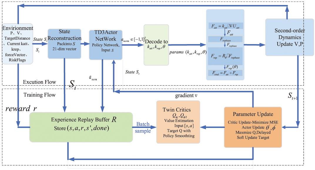Fig. 2. TD3-APF algorithm architecture diagram.

During the training process, the UAV continuously interacts with the environment, acquiring observational information about the current system provided by the environment. Subsequently, the policy network outputs actions based on this state and converts them into adjustable quantities usable by the controller through an intermediate mapping or decoding process. Under the influence of these adjustable quantities, control commands for the UAV are generated, state updates are performed, and rewards are obtained. The experience gained from these interactions is written into a replay pool to support subsequent training and learning. During the training phase, the system samples data from the replay pool and generates learning signals through value evaluation and stabilization mechanisms. Then, it gradually optimizes the policy and evaluation networks through gradient updates and simultaneously updates the target network.

B.DESIGN OF FORMATION CONTROL ALGORITHM

As for the improvement of the APF algorithm, we physicalize the design process of the control law, specifically designing navigation force, obstacle avoidance force, and coordination force to achieve the formation flight task of UAVs [25]. Under the second-order dynamic integrator model, the control input $u_{i}$ of the UAV represents its acceleration, which is regarded as the resultant external force acting on the UAV. The control law is designed using the virtual force synthesis method, decoupling the complex formation flight task into three independent mechanical components: navigation, obstacle avoidance, and coordination. The final comprehensive control command is generated by superimposing vectors. The specific process is shown in Fig. 3.

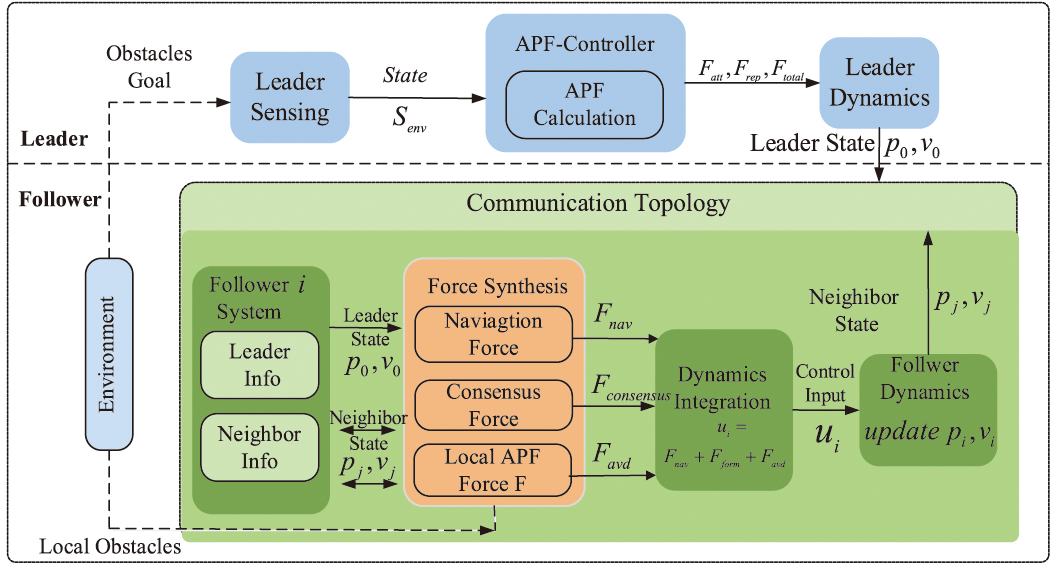Fig. 3. UAV formation control law algorithm APF-Consensus.

For the construction of the virtual force component $i$ ( $i \in V_{F}$ ) of any follower UAV in the formation, the resultant external force $u_{i}$ it experiences is composed of the following three parts:

u_{i} = F_{nav, i} + F_{avd, i} + F_{form, i}

(17)

The navigation and traction components are primarily responsible for driving the follower to track the trajectory of the leader node 0. The position error of the follower $i$ relative to the leader is defined as $e_{p, i 0} = p_{i} - p_{0} - δ_{i 0}$ , and the velocity error is defined as $e_{v, i 0} = v_{i} - v_{0}$ . The traction force is designed as:

F_{nav, i} = - d_{i} [k_{p} (p_{i} - p_{0} - δ_{i 0}) + k_{v} (v_{i} - v_{0})]

(18)

where

d_{i}

is the traction coefficient, and if

i

can be observed or is related to the lead aircraft, then it is 1, otherwise it is 0.

δ_{i 0}

is the expected relative position.

The component of obstacle avoidance repulsive force is primarily responsible for ensuring flight safety, originating from the repulsive force field gradient in the APF [26]. A high potential field exists around obstacles, with potential energy inversely proportional to distance, generating a repulsive force directed toward the UAV. Let $ρ_{i j}$ be the surface distance from the UAV $i$ to the obstacle $k$ , and $n_{i k}$ be the unit vector pointing from the obstacle toward the UAV. The repulsive force is designed as follows:

F_{a v d, i} = \sum_{k \in O} η (\frac{1}{ρ_{i k}} - \frac{1}{ρ_{0}}) \frac{1}{ρ_{i k}^{2}} n_{i k}

(19)

This component of formation synergy is responsible for maintaining the geometric configuration among followers, incorporating consistency theory to prevent formation loosening or internal collisions. There is a mutual interaction and coupling force between all neighboring nodes within the formation. Based on the second-order consensus protocol, UAV $i$ need to utilize information from neighboring node $j$ to eliminate relative position and velocity errors:

F_{f o r m, i} = \underset{j \in N_{i}}{- \sum} a_{i j} [k_{p} (p_{i} - p_{j} - δ_{i j}) + k_{v} (v_{i} - v_{j})]

(20)

where

δ_{i j} = δ_{i 0} - δ_{j 0}

represents the expected spacing between follower

i

and

j

, and

a_{i j}

denotes the weight of the adjacency matrix.

{\tilde{p}}_{i 0} = p_{i} - p_{0} - δ_{i 0}

denotes the position error relative to the navigator.

{\tilde{p}}_{i j} = p_{i} - p_{j} - δ_{i j}

denotes the position error relative to the neighbor.

The above three mechanical components are linearly superposed and organized into the matrix expression form of algebraic graph theory. Finally, the i-th UAV’s final control law is obtained:

u_{i} = \underset{①}{(- d_{i} k_{v} (v_{i} - v_{0}) - \sum a_{i j} k_{v} (v_{i} - v_{j}))} + \underset{②}{(- d_{i} k_{p} {\tilde{p}}_{i 0} - \sum a_{i j} k_{p} {\tilde{p}}_{i j})} + F_{a v d, i}

(21)

where

①

is the speed component and

②

is the position component.

C.STABILITY ANALYSIS OF FORMATION CONTROL LAW

First, in the APF, the repulsive force $F_{avd}$ is the negative gradient of the position-dependent potential field function $F_{avd} (p) = - \nabla_{p} U_{rep} (p)$ , which indicates that $F_{avd}$ is a conservative force. Conservative force work depends only on the starting and ending positions, independent of the path, and the corresponding potential energy $U_{rep}$ is a scalar field. This means that the repulsive force potential energy is additive when constructing the Lyapunov function, that is, the total energy function of the system. Only the repulsive force potential energy is directly superimposed on the original formation error potential energy, and a new energy function can be constructed without destroying the original system structure.

In order to prove the stability after adding repulsive force, an augmented Lyapunov candidate function $V_{aug}$ including formation synergy potential energy, obstacle avoidance repulsive force potential energy, and system kinetic energy is constructed:

V_{a u g} (E_{p}, E_{v}) = \frac{1}{2} k_{p} \underset{①}{E_{p}^{T} (H \otimes I) E_{p}} + \sum_{i = 1}^{N} \underset{②}{U_{r e p} (p_{i})} + \frac{1}{2} \underset{③}{E_{v}^{T} E_{v}}

(22)

where

①

represents formation synergy potential energy,

②

represents obstacle avoidance repulsive force potential energy, and

③

represents system kinetic energy.

Since $H$ is an M-matrix and contains a spanning tree, $H$ is positive definite, meaning $V_{form} \geq 0$ . Repulsive force potential energy $U_{rep} (p)$ is defined as the inverse square or truncated quadratic form of distance, which is naturally $V_{obs} \geq 0$ . The kinetic energy term is clearly nonnegative. Therefore, $V_{aug}$ is positive definite and radially unbounded, meeting the basic conditions of Lyapunov functions.

The total time derivative of $V_{aug}$ with respect to time $t$ is given as:

{\dot{V}}_{a u g} = \frac{d V_{f o r m}}{d t} + \frac{d V_{o b s}}{d t} + \frac{d V_{k i n}}{d t} = k_{p} E_{p}^{T} H E_{v} - k_{p} E_{v}^{T} H E_{p} + {(- F_{a v d}^{g l o b a l})}^{T} E_{v} + E_{v}^{T} F_{a v d}^{g l o b a l} - k_{v} E_{v}^{T} (H \otimes I) E_{v} = - k_{v} E_{v}^{T} (H \otimes I) E_{v}

(23)

The final derivative form is obtained as:

{\dot{V}}_{a u g} \leq - k_{v} λ_{m i n} (H) {‖ E_{v} ‖}^{2} \leq 0

(24)

The above formula shows that the addition of force does not destroy the stability. The repulsive force $F_{avd}$ is used as the driving force in the dynamic equation, but it is shown as potential energy release in the derivation of the potential energy function. The two are precisely canceled out in the Lyapunov derivative.

D.IMPROVEMENT OF TD3-APF ALGORITHM

The reward function is a core component of reinforcement learning, and the rationality of its design directly determines the convergence speed and ultimate performance of the policy [27]. This study, tailored to the characteristics of UAVs and potential field methods, designs a hybrid reward function that incorporates graded risk penalties, active ablation for stagnation, and action smoothness constraints. Total reward $r_{t}$ is defines as:

r_{t} = r_{prog} + r_{risk} + r_{stag} + r_{smooth}

(25)

The progress reward $r_{prog}$ guided by potential energy is defined as:

r_{prog} = λ_{1} (d_{t - 1}^{goal} - d_{t}^{goal}) - λ_{time}

(26)

Dual-threshold graded risk penalty $r_{risk}$ is defined as:

r_{r i s k} = {\begin{cases} - w_{1} {(1 - \tilde{d})}^{2}, & R_{i n} < d < R_{o u t} \\ - w_{2} {(1 - \tilde{d})}^{4} - \frac{w_{3}}{d + 0.1}, & d < R_{i n} \end{cases}

(27)

Stagnation detection and active ablation reward $r_{stag}$ is defined as:

To address the issue of UAVs oscillating around the original position due to the APF’s tendency to get stuck in local minima, an active guidance mechanism is introduced. This mechanism maintains a sliding window and calculates the total distance of position changes within the window. If the distance is less than a threshold, it is determined to be stuck. Once stagnation is detected, a single heavy penalty is immediately imposed, and rewards are dynamically reshaped.

Action smoothness regularization $r_{smooth}$ is defined as:

r_{smooth} = - λ_{dir} {‖ a_{t} - a_{t - 1} ‖}^{2}

(28)

This term penalizes large differences between consecutive actions $a_{t}$ at and $a_{t - 1}$ , encouraging smoother, more stable control inputs and reducing abrupt control changes that could degrade system performance or cause instability.

IV.EXPERIMENTAL RESULTS AND DISCUSSION

A.EXPERIMENTAL ENVIRONMENT AND PARAMETER SETTINGS

The simulation experiment in this chapter is conducted in an environment with Windows 10, Python 3.8, and TensorFlow 1.14.0. Based on the modification and adaptation of the gym framework using pygame, the simulation design and experiment of multi-UAV formation flight control are carried out.

The task scenario involves six UAVs, utilizing a leader–follower architecture, specifically comprising one leader UAV and multiple follower UAVs, as illustrated in Fig. 4.

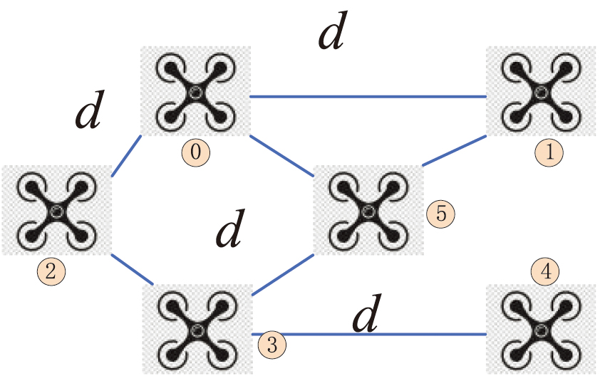Fig. 4. Experimental formation topology.

In Fig. 4, UAV No. 5 serves as the lead UAV, while the other UAVs act as followers.

The simulation scenario for multi-UAV formation flight control based on pygame is shown in Fig. 5.

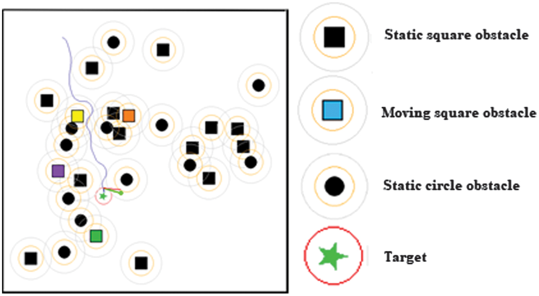Fig. 5. Task scenario composition.

The specific task setting is as follows: the simulation step size for the UAV formation flight task is designed to be $Δ t = 0.1 s$ , and the task boundary length is 600 * 600 m. The parameters adopted by the UAV are shown in Table I.

Table I. UAV parameters description

Parameter	Value	Parameter	Value
Initial speed	0 m/s	Perception range	60 m
Initial heading angle	1.5π–2π	Angular speed acceleration	2 rad/s²
Maximum speed	30 m/s	Maximum acceleration	10 m/s²

The radius of circle obstacle is 15 m, and the side length of square obstacle is 15 m as well. As for the moving obstacle, the moving speed is 5 m/s.

Parameter settings corresponding to APF are shown in Table II.

Table II. Parameters of APF

Parameter	Value	Parameter	Value
Attractive force factor	0.3–1.5	Attractive force limitation	800
Repulsive force factor	50–300	Repulsive force limitation	1000
Warning range	50 m	Hazardous action range	30 m

B.SINGLE UAV PATH PLANNING BASED ON TD3

The parameter settings for the TD3 algorithm encompass the configuration of the experience replay pool, learning rates for the actor and critic, among others. Detailed parameter settings are presented in Table III.

Table III. Parameters of TD3 algorithm

Parameter	Value	Parameter	Value
Maximum capacity of experience replay pool	200000	Action network learning rate	0.001–0.003
Sampling size	128	Value network learning rate	0.001–0.003
Maximum number of rounds	1500	Soft update rate	0.01
Maximum step length per round	800	Discount factor	0.95
Warm-up step length	5000	Policy noise	0.1

Based on the description of the experimental scenario mentioned above and the descriptions of the TD3 and APF algorithms, training and validation work for dynamic parameter adjustment of APF based on TD3 were conducted. The reward curve is shown in Fig. 6.

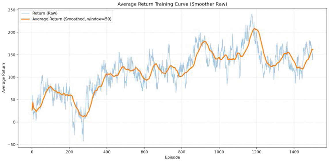Fig. 6. TD3-APF reward training curve.

In Fig. 6, the x-axis represents the number of training episodes, and the y-axis represents the average reward obtained by a single UAV every 50 training episodes. At the beginning of training, due to the control ability of traditional algorithms, they also possess a certain ability to obtain rewards during the exploration phase. However, their ability to obtain rewards is mainly concentrated in a certain range and cannot be further improved. After the training officially begins, the UAV starts to perceive the environment and continuously interacts with it, enhancing its strategy and acquiring the ability to apply the APF method. The UAV’s phased acquisition of perception and interaction abilities with the environment, as well as its gradual improvement in reward acquisition, indicates that its strategy can continuously learn and acquire better adaptability.

The success rate is shown in Fig. 7.

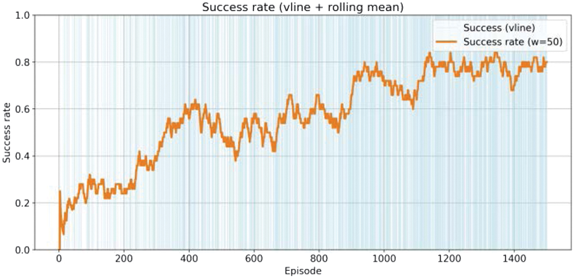Fig. 7. TD3-APF success rate curve.

Testing under the TD3 algorithm: After completing the APF training under the TD3 algorithm, the model was tested. Two hundred scenarios in the validation environment were used for testing, and their success rate, step length, and performance under special scenarios were analyzed. As shown in Fig. 8, the success rate was 84%, the failure rate was 16%, of which 2.5% was due to out-of-bounds issues, and the collision rate was 13.5%. There were no task failures caused by timeouts in the experimental scenarios.

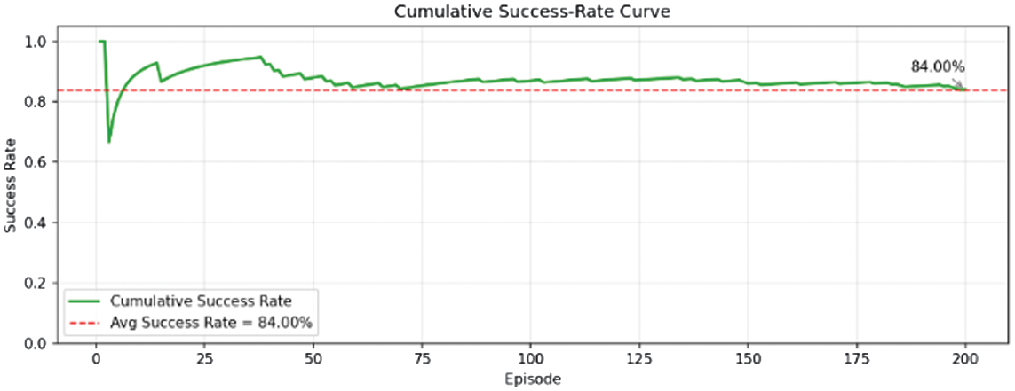Fig. 8. TD3-APF cumulative success rate curve.

Typical scenarios are selected from the test scenarios for description, namely Scenario 1, Scenario 2, Scenario 3, and Scenario 4. Fig. 9 illustrates several escape scenarios of the UAV under potential local minima.

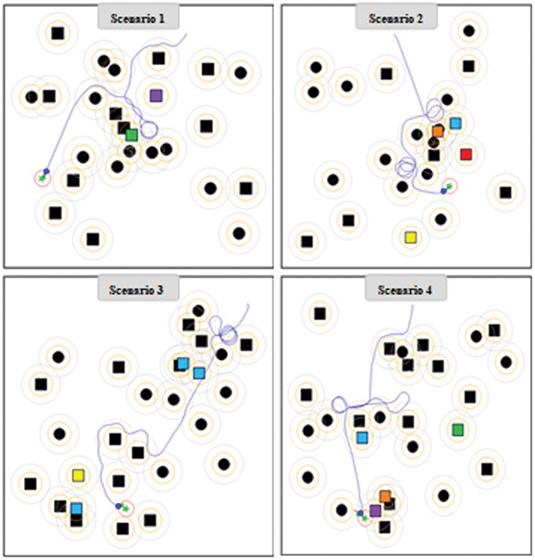Fig. 9. Test scenarios trajectory.

In Scenario 1, the UAV gets trapped in a local dilemma near a green obstacle. After escaping from the local dilemma, it continues to move along the tangent direction of the potential field without falling into a local minimum again and finally completes the escape after finding an exit. In Scenario 2, the UAV performs two escape maneuvers before reaching the target point. It quickly escapes at the first escape point, and at the second escape point, it simultaneously experiences repulsive forces from three obstacles, causing it to enter and exit two local dilemmas back and forth while deviating from the target direction. In Scenario 3, the UAV starts in a near-U-shaped trap, searching for potential exits. Through the combined effects of adjusting attractive and repulsive forces, as well as the direction of the repulsive force, it passes through previously inaccessible areas and escapes from symmetric obstacle dilemmas twice before reaching the target point.

C.IMPROVED FORMATION FLIGHT UNDER THE APF ALGORITHM

In the scenario of UAV formation operation, the size of the scenario is set to 600 * 600 m. Considering that multi-UAVs require a lot of formation maintenance during formation flight, the difficulty requirement of obstacles in the scene is weakened. Corresponding dynamic and static obstacles are randomly generated in the scene.

1).VERIFICATION OF FORMATION CONTROL LAW INTEGRATING APF

First, the formation error of a formation is defined as follows:

e_{x} = (p_{x, j} - p_{x, i}) - (δ_{x, j} - δ_{x, i})

(29)

e_{y} = (p_{y, j} - p_{y, i}) - (δ_{y, j} - δ_{y, i})

(30)

After sorting:

{LocalError}_{i j} = (p_{j} - p_{i}) - (δ_{j} - δ_{i})

(31)

where

p_{j} - p_{i}

is the actual relative position vector of the neighbor

j

relative to itself

i

δ_{j} - δ_{i}

is the expected relative position vector of the neighbor

j

relative to itself

i

The formation error in the form of root mean square error (RMSE) is finally calculated:

E_{R M S E} = \sqrt{\frac{1}{| E |} \sum_{(i, j) \in E} {‖ (p_{j} - p_{i}) - (δ_{j} - δ_{j}) ‖}^{2}}

(32)

where

| E |

is the total number of edges existing in the communication topology network, only counting the pairs of UAV nodes with communication connections. Formation error is not only a geometric distance but also a perception error in the control algorithm. This judgment ensures that the evaluation metric is completely consistent with the input of the consensus control algorithm, and the control law only optimizes the connected edges, so the error is also only calculated for the connected edges. The RMSE can reflect the average degree of deformation of each inter-node connection.

We design three scenarios. First, when there are basically no obstacles in the path connecting the starting point and the end point, and the APF is basically not functioning, it is tested whether the UAV formation can maintain the desired formation. Second, when there are several obstacles on the line connecting the starting point and the end point, it is tested whether it can complete obstacle avoidance and maintain the formation after avoiding the obstacles. Finally, when there are symmetrical obstacles between the starting point and the end point, it is tested whether the formation can complete obstacle avoidance and whether it can be restored to the desired formation after avoiding the obstacles.

2).FORMATION FLIGHT EXPERIMENT IN A BARRIER-FREE ENVIRONMENT (SIMPLE SCENARIO)

Figure 10 depicts the flight trajectory of a UAV formation in a simple environment, which can smoothly maintain its formation and fly toward the target point. Figure 11 illustrates the flight error of the UAV formation during formation flight. Due to the initial state of the UAV formation not reaching the desired formation at the initial position, there is an initial formation error. In the early stage, the formation quickly completes the formation-building process near a 25-step length, achieving a low formation error. Subsequently, the formation flies toward the target point. In the scenario where there are no obstacles on the path, the UAV formation maintains a low formation error throughout and converges to 0 after reaching the end point and several steps, thereafter, fully converg to the desired formation.

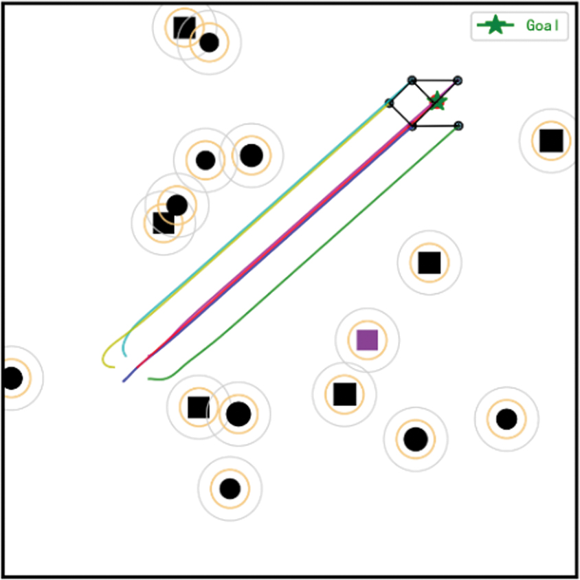Fig. 10. UAV formation flight trajectory with few obstacles.

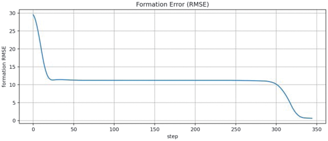Fig. 11. Formation error variation graph.

In the initial stage of UAV formation, the initial position of the UAV members deviates from the expected position of the UAV, and there is a large variation in the control input of the UAV members. After 25 steps, the UAV’s formation error reaches a low level. As shown in Figs. 12 and 13, at around 50 steps, the UAV achieves velocity consistency. There is a lag in the convergence of the formation velocity to the common velocity of the formation, but after achieving velocity consistency, UAV formation basically achieves long-term consistency in position and velocity without interference.

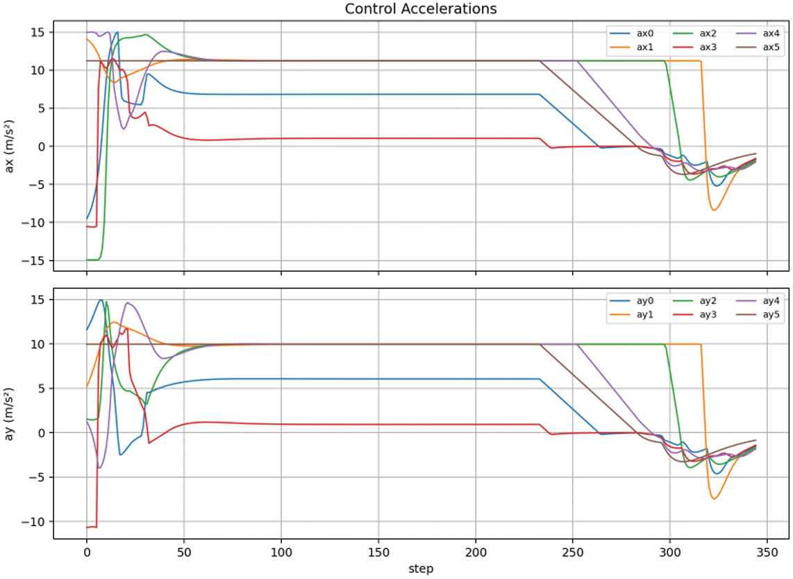
Fig. 12. Control accelerations of UAV formation.

Fig. 13. Control velocities of UAV formation.

3).FORMATION FLIGHT EXPERIMENT UNDER SEVERAL OBSTACLES

Figures 14 and 15 show the process of the UAV formation quickly completing its formation construction near a 25-step length, achieving a relatively low formation error. At around 50 steps, the formation flies toward the target point and encounters a static obstacle. Under the influence of the repulsive force field, the UAV formation moves away from the obstacle, during which the formation error rapidly increases. After escaping from the obstacle, its formation error gradually decreases. At around 225 steps, it encounters a green dynamic obstacle. While completing the avoidance maneuver, its formation error further increases, and after reaching the end point and several steps later, the formation error converges to a lower level, converging to the desired formation.

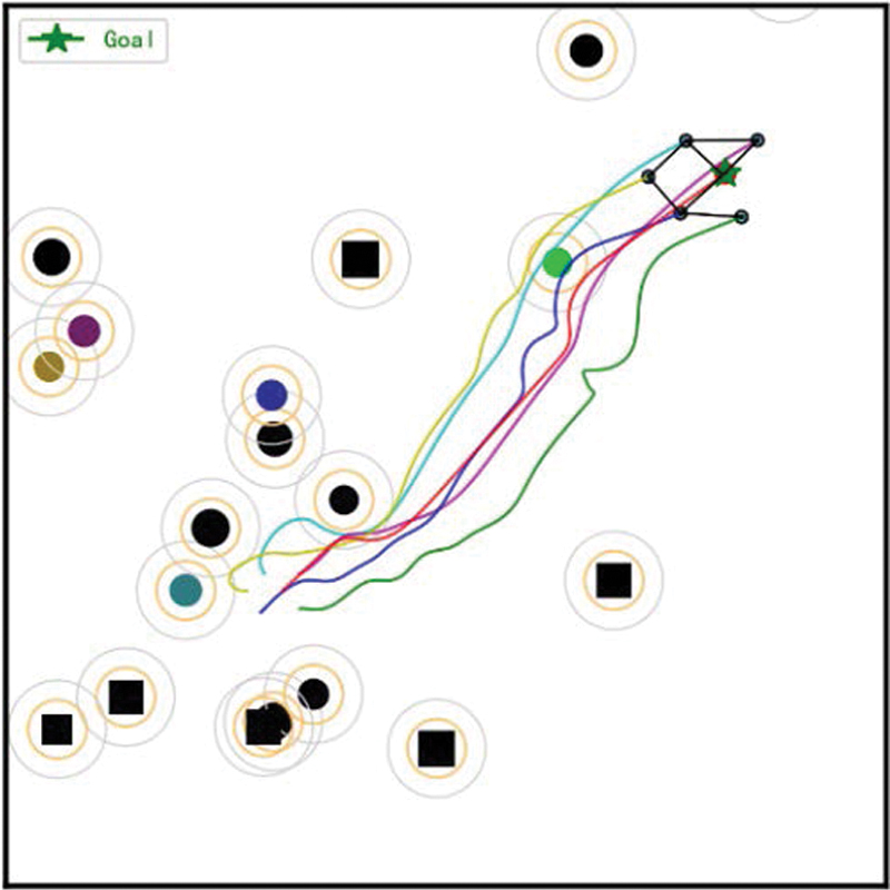Fig. 14. UAV formation flight trajectory with several obstacles.

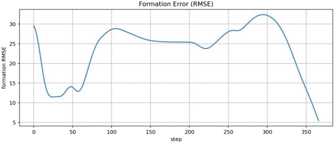Fig. 15. Formation error variation graph.

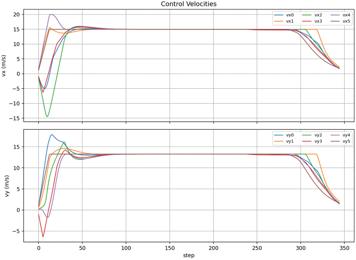
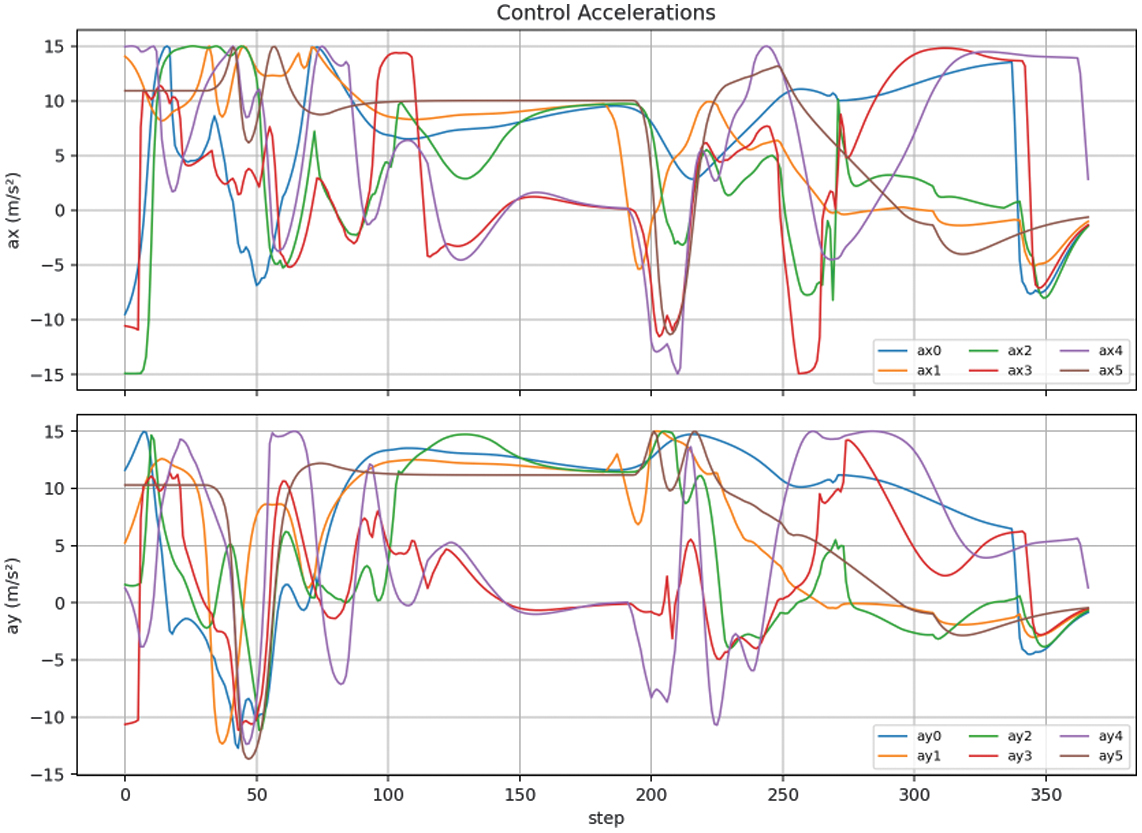
As shown in Figs. 16 and 17, during the initial formation phase and obstacle avoidance phase, there are significant changes in the control inputs for the UAV members during the long-term periods of 0–25, 50–100, and 225–300 steps, respectively. Throughout the overall operation process, the UAV formation is able to complete obstacle avoidance while maintaining a certain formation and recover to the desired formation after the avoidance is completed.

Fig. 16. Control accelerations of UAV formation.

Fig. 17. Control velocities of UAV formation.

4).FORMATION FLIGHT EXPERIMENT IN LOCAL MINIMA DILEMMA

In this scenario, there may be a situation where a symmetrical obstacle is generated in the middle of the line connecting the starting point and the target point. In this case, the UAV leader uses the APF algorithm for driving. If it falls into the repulsive field near the symmetrical obstacle, it will produce local oscillations and cannot escape from the local dilemma.

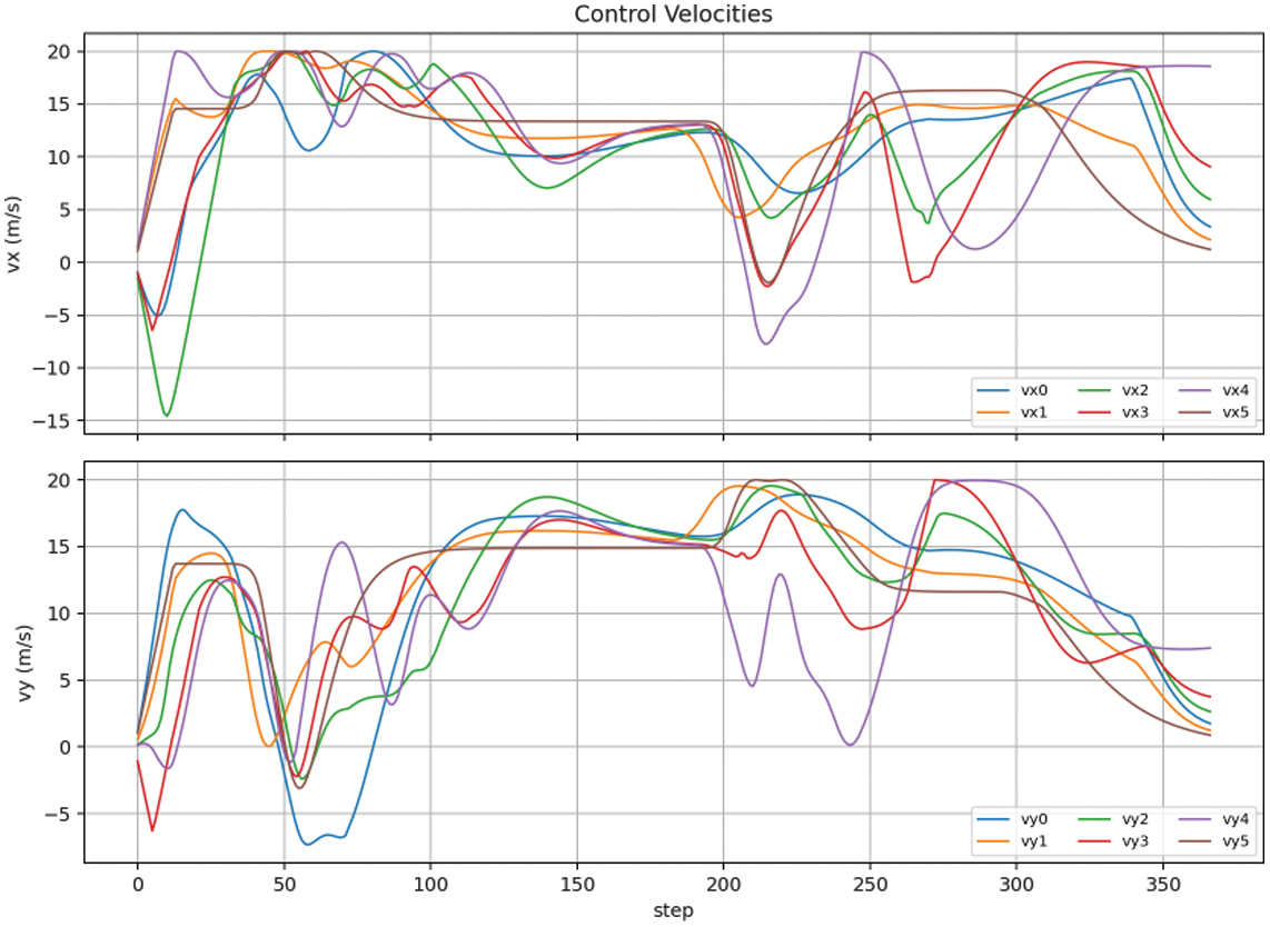
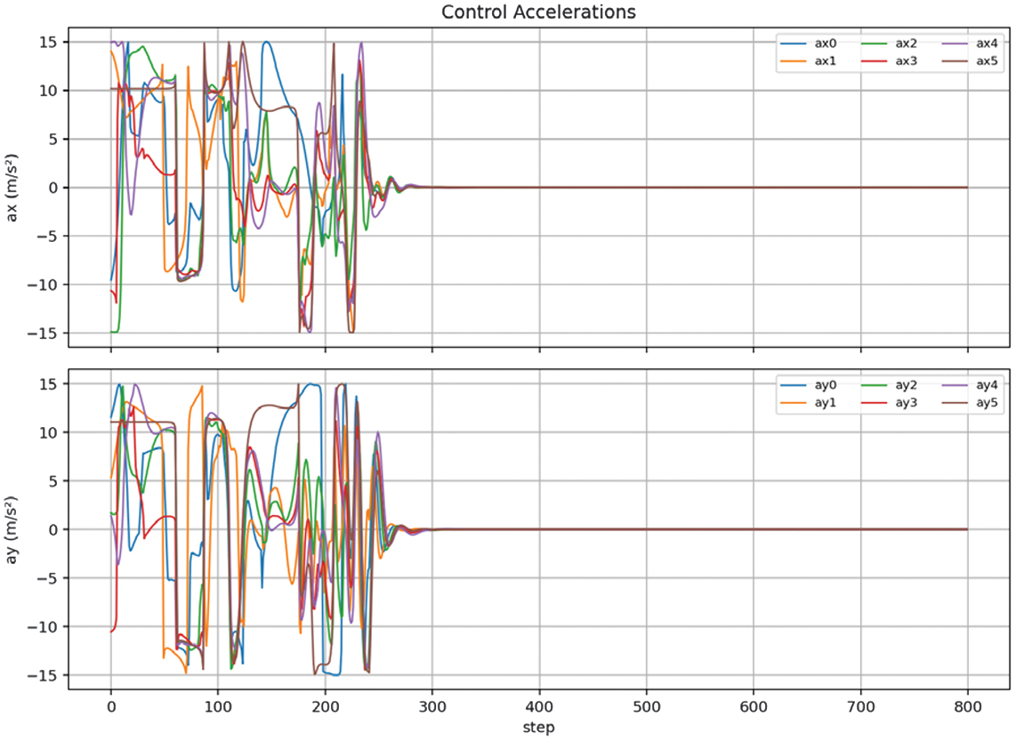
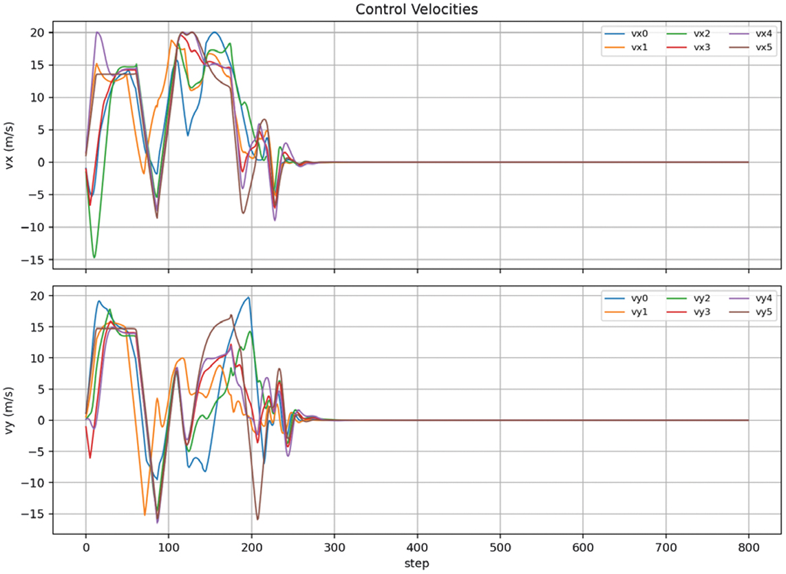
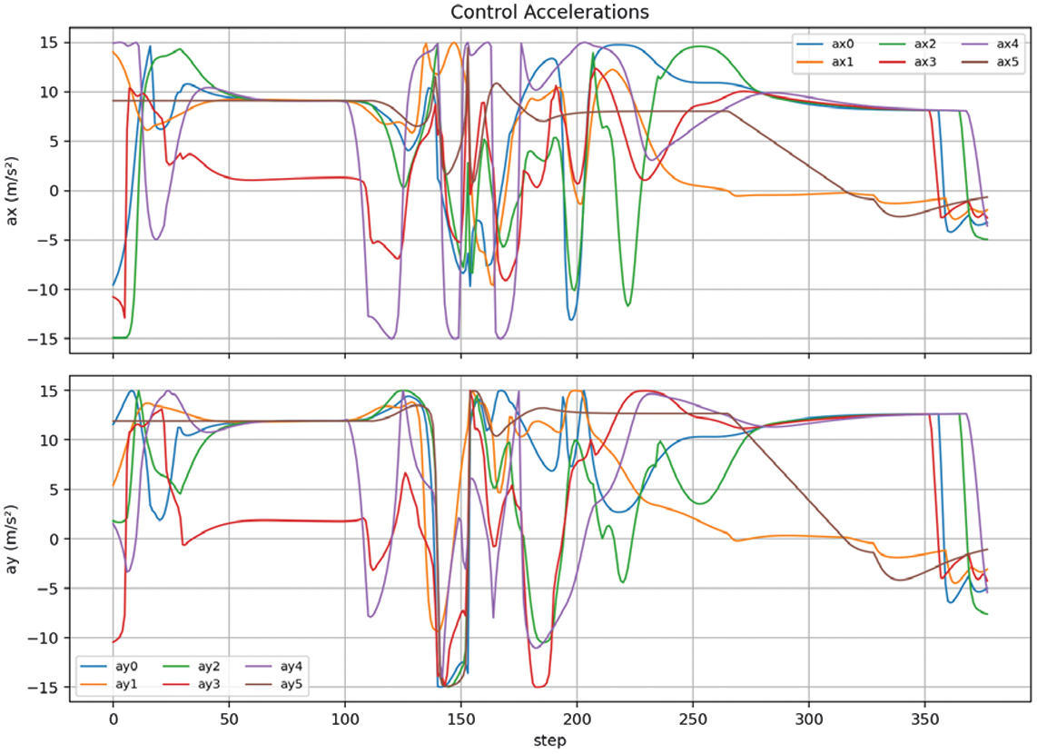
As shown in Figs. 18 and 19, the leader UAV falls into local oscillation, eventually reaching a point of force balance where no control input is generated. The UAV falls into a potential trap. When the leader UAV falls into the potential trap, the follower UAVs still fly toward the desired position corresponding to the leader UAV. When the position and velocity attributes align with those of the leader UAV, the control input of the follower UAVs also approaches 0 due to the influence of the control law. Since their positions are near obstacles, the follower UAVs generate a weak repulsive force within the range of the repulsive force, and the entire UAV formation is at the edge of the obstacle, reaching equilibrium. Figs. 20 and 21 illustrate the formation acceleration and velocity of UAV formation separately.

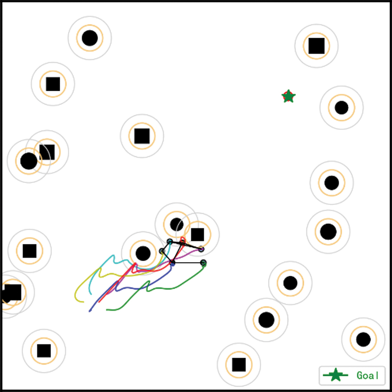Fig. 18. Local dilemma graph of UAV formation.

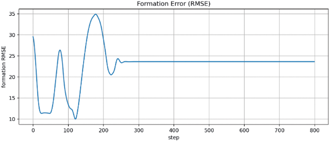Fig. 19. Formation error variation graph.

Fig. 20. Control accelerations of UAV formation.

Fig. 21. Control velocities of UAV formation.

5).VERIFICATION OF FORMATION CONTROL LAW COMBINING TD3-APF

For the local dilemmas in the scenario, we apply the TD3-APF dynamic parameter adjustment method to the path planning of the leader UAV, testing whether it can overcome the dilemma in the corresponding scenario environment and improve the flight performance of the entire formation.

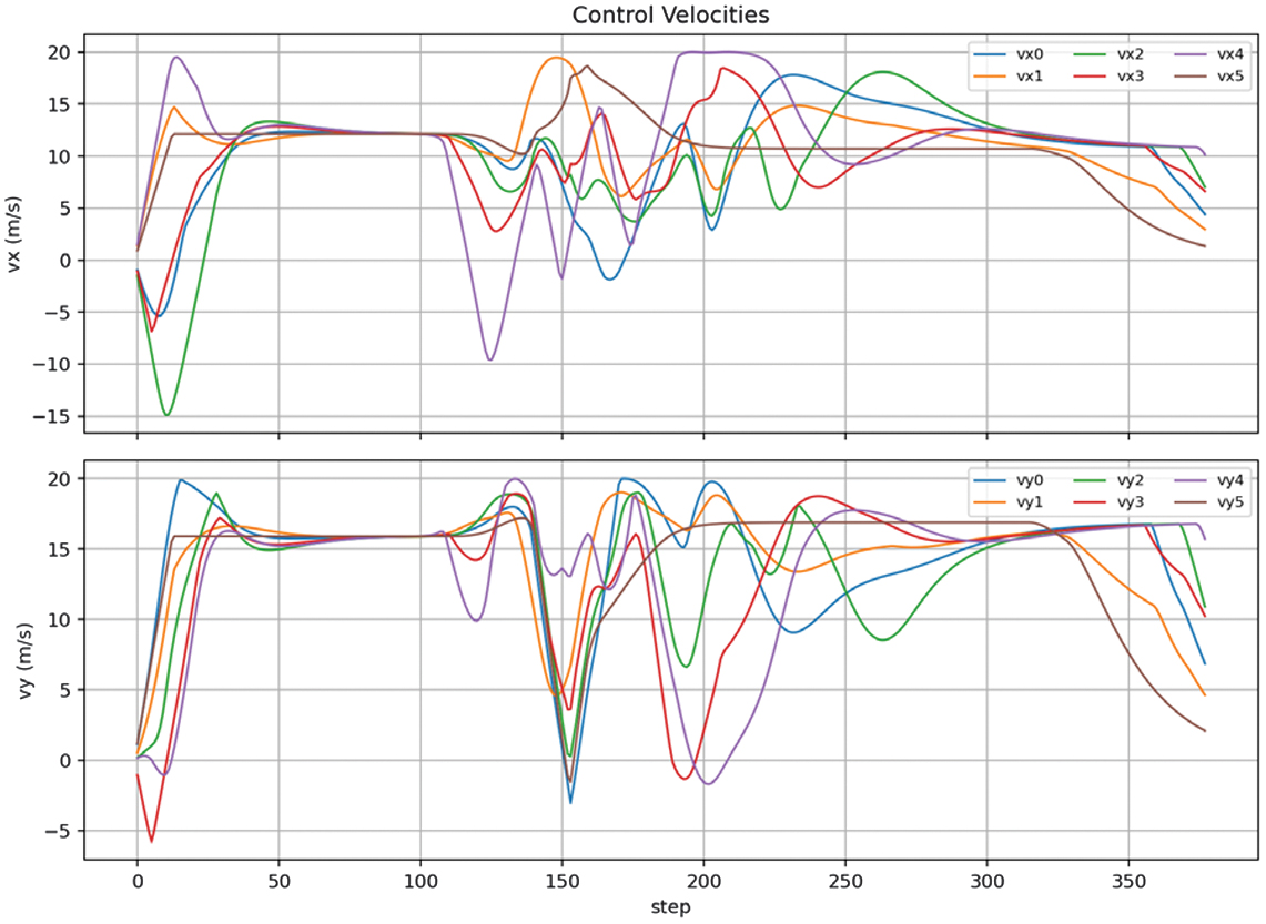
Figure 22 illustrates the flight trajectory of the UAV formation under the TD3-APF algorithm employed by the lead UAV. In Fig. 23, the UAV formation, with a step length of 125, experiences a local predicament as the lead aircraft navigates through it. Under the guidance of the lead aircraft, some of the UAVs in the formation follow the lead aircraft’s trajectory, passing through the center of the symmetrical obstacle and reaching the target point. During the initial phase without obstacles, the UAV formation can still quickly converge to the desired formation and achieve velocity consistency and recover its formation after avoiding obstacles. Figs. 24 and 25 illustrate the formation acceleration, and velocity of UAV formation separately.

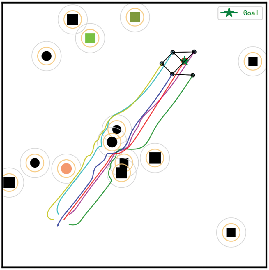Fig. 22. Trajectory graph of UAV formation in a symmetric obstacle scenario.

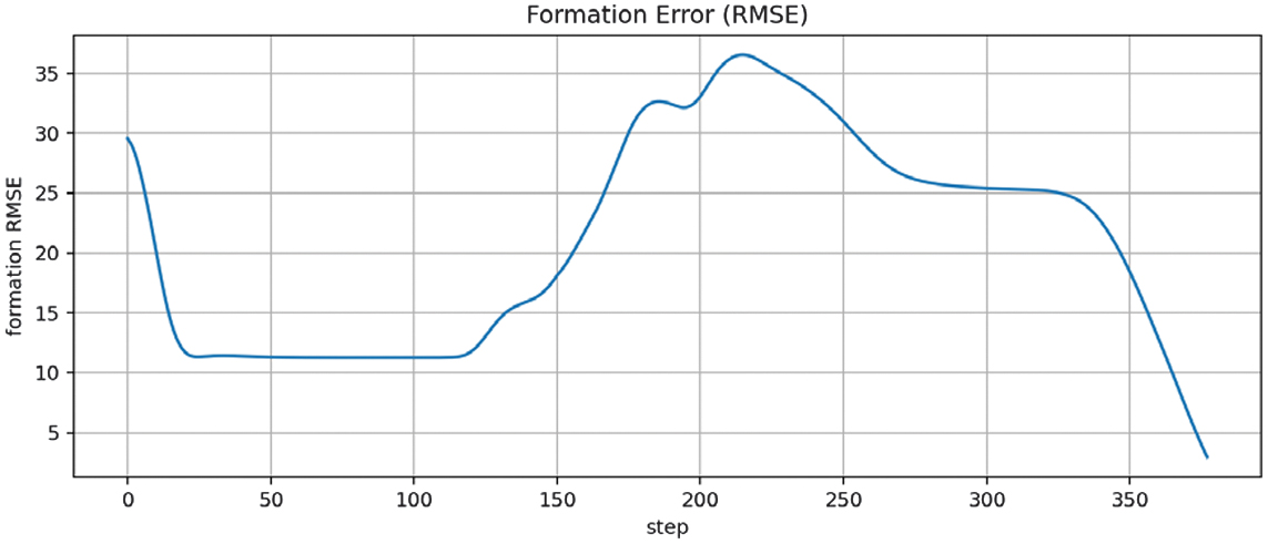Fig. 23. Formation error variation graph.

Fig. 24. Control accelerations of UAV formation.

Fig. 25. Control velocities of UAV formation.

V.CONCLUSION

This paper implements multi-UAV formation flight based on the APF algorithm and consensus algorithm. It improves the APF algorithm through the DRL algorithm TD3, applying it to the flight control of the leader UAV to enhance the formation flight capability. First, by designing the formation control law and analyzing its stability, the stable formation flight, obstacle avoidance, and ability to reach the target point of the UAV formation are achieved. Then, the TD3 algorithm dynamically adjusts the parameters of the APF algorithm to overcome its local minima problem, improving the success rate of single UAVs. Finally, its impact on the overall formation flight effect in the leader UAV of the UAV formation is verified. By combining TD3 and APF, the improved APF algorithm enhances its ability to solve local minima problems in both single and formation flight applications of the leader UAV.

Nevertheless, this research has certain limitations. The proposed method is developed on a simplified 2D kinematic model without considering detailed dynamics, actuator lag, aerodynamic effects, or external disturbances. All experiments are conducted in simulation with regular obstacles and fixed leader–follower topology, without involving 3D terrain, communication constraints, or real-world uncertainties. In addition, the computational cost of TD3 may restrict its direct deployment on embedded aerial platforms, and hardware validation has not yet been implemented.

Future research will focus on lightweighting the learning algorithm for onboard real-time execution, extending the framework to 3D scenarios with disturbance rejection and adaptive topology switching, and conducting hardware-in-the-loop and real-flight verification to improve engineering practicability. Further efforts will also be devoted to enhancing robustness under communication interruption, fault tolerance, and multi-task collaborative missions so as to promote the deployment of learning-based formation control in practical UAV swarm systems.

UAV Formation Control Based on Deep Reinforcement Learning and Dynamic Artificial Potential Field

I.INTRODUCTION

II.PROBLEM FORMULATION AND SYSTEM MODELING

A.PROBLEM FORMULATION

B.SYSTEM MODELING

1).DEFINITION OF STATE SPACE

2).DISCRETE TIME KINEMATIC EQUATION

3).PHYSICAL CONSTRAINTS AND NONHOLONOMIC CONSTRAINTS

C.STATE SPACE CONSTRUCTION

1).STATE SPACE

2).COMPOSITE PARAMETER ACTION SPACE

III.PROPOSED HIERARCHICAL META-CONTROL METHODOLOGY

A.DISCRIPTION OF ALGORITHM

B.DESIGN OF FORMATION CONTROL ALGORITHM

C.STABILITY ANALYSIS OF FORMATION CONTROL LAW

D.IMPROVEMENT OF TD3-APF ALGORITHM

IV.EXPERIMENTAL RESULTS AND DISCUSSION

A.EXPERIMENTAL ENVIRONMENT AND PARAMETER SETTINGS

B.SINGLE UAV PATH PLANNING BASED ON TD3

C.IMPROVED FORMATION FLIGHT UNDER THE APF ALGORITHM

1).VERIFICATION OF FORMATION CONTROL LAW INTEGRATING APF

2).FORMATION FLIGHT EXPERIMENT IN A BARRIER-FREE ENVIRONMENT (SIMPLE SCENARIO)

3).FORMATION FLIGHT EXPERIMENT UNDER SEVERAL OBSTACLES

4).FORMATION FLIGHT EXPERIMENT IN LOCAL MINIMA DILEMMA

5).VERIFICATION OF FORMATION CONTROL LAW COMBINING TD3-APF

V.CONCLUSION

CONFLICT OF INTEREST STATEMENT

REFERENCES