JAIT

I.INTRODUCTION

The Internet of Things (IoT) is progressively vulnerable to safeguarding attacks, which are gaining popularity. These attacks are present in multiple behaviors and target anomalous resources, affecting multiple IoT devices [1,2]. Designing intrusion-resistant IoT networks and securing IoT devices have become crucial for protecting data [3]. Major technologies are 5G advancement, cloud computing, fog computing, and artificial intelligence in IoT form the backbone of the digital world [4]. A common challenge is resource limitation, which refers to the power capacity and computing ability that delay the complex intrusion detection system (IDS) deployment across IoT devices [5]. Additionally, numerous devices are associated with the Internet, and hackers are frequently developing new attack methods [6]. Developing a more precise IoT-IDS system requires the combination of maximum robust models [7]. Recently, deep learning (DL) methods are used for detecting cyberattacks because of their capability to address large volume of intricate patterns of network data [8]. These models have evolved to incorporate dynamic IoT contexts and emerging attack techniques [9]. To effectively detect new anomalies, these models continually learn new patterns while improving overall performance [10].

For this reason, a DL-based intrusion detection method is proposed in this research to classify IoT device network attacks [11]. Recent studies focus on spatiotemporal features in traffic data, capturing the interdependencies between multiple dimensions in IoT data [12]. Several studies identified the most efficient intelligent IDS for IoT environments [13]. However, some techniques are used on small datasets, where time and space complexity become concerns due to the high dimensionality and complexity of IoT data [14]. Parallelized DL-based models are employed to address these challenges, improving scalability and processing efficiency when handling high-dimensional data [15]. IoT comprises an interconnected network of sensors, software, computing devices, smart devices, and actuators [16]. Reliable and accurate data exchange is essential in IoT networks, as attackers aim to compromise system integrity and steal information [17,18]. Due to the variability of protocols and IoT devices, attacks can easily disrupt IoT networks and threaten their security [19]. These malicious activities can continue even deployment, reducing system reliability [20]. The contributions of this research are as follows:

•One-dimensional convolutional neural network (1D-CNN) method helps automatically extract essential spatial features from sequential network traffic, enabling high-speed detection.
•The parallel interaction attention (PIA) mechanism considers the network by processing spatial features and temporal dependencies simultaneously, rather than sequentially. Weights are assigned to both temporal and spatial features across parallel streams to isolate important attack patterns from background noise.

The remaining part of this paper is organized as follows: Literature survey is described in section II, proposed methodology is presented in section III, results and discussion is represented in section IV, and section V concludes overall research.

The remainder of this paper is organized as follows: section II presents a literature review of IDS in IoT. The proposed methodology is explained in section III, and section IV represents experimental results and discussion. Section V concludes overall research.

II.LITERATURE REVIEW

Traditional research methods, along with their advantages and limitations, are summarized in IDS detection.

Maoudj S.E. et al. [21] developed a 1-DCNN to enhance IDS in IoT networks. A proposed model was used to predict a single outcome for the minority class with network traffic. Additionally, another 1-DCNN was trained specifically on this minority, and this second prediction was performed only if the initial minority model classified the output as belonging to the minority class. A class weight technique was also employed to ensure balanced learning in the models. However, detection rates for some minority classes remained low due to the integrated effects of class overlapping and imbalanced data.

Jablaoui R. et al. [22] introduced a hybrid DL-based model that combined gated recurrent unit (GRU) and CNN to improve IDS. In network traffic data, spatial features are captured by the CNN, while the GRU modeled temporal dependencies, making this combination effective for detecting complex and dynamic intrusions in IoT environments. Nevertheless, the CNN technique faced a high rate of misclassified attacks, indicating challenges in accurately differentiating between classes.

Wang X. et al. [23] implemented a DL-based model such as a conditional tabular generative adversarial network (CTGAN) for IDS detection. The goal was to increase the volume of data for smaller classes, address data imbalance issues, and improve the overall intrusion detection network. However, the CTCAN still needed to improve its performance in handling missing data values.

Thaljaoui A. et al. [24] demonstrated a hybrid DL approach combining CNN and Long Short-Term Memory (LSTM) with hyperparameter optimization using Bayesian for IoT intrusion detection. Dimensional features are extracted by the CNN and LSTM in network traffic data. However, the CNN-LSTM was sensitive to hyperparameter selection, where diverse parameter tuning and initialization affected the consistency and reproducibility of results.

Zhang H. et al. [25] established an ensemble model for IDS detection in IoT. The main objective was to identify IDS attacks in IoT by addressing existing reviews of IDS and exploring DL applications for network security. An ensemble learning and a total of 21 neural network models were used and trained. However, the research highlighted the model’s effectiveness and mainly relied on parameter tuning and computational resources, which limited the practical deployment of IoT.

Shah H. et al. [26] introduced an enhanced approach for estimating gaps and predicting missing values in real-time communication systems. This approach reconstructed and predicted missing values using the imputed missing value-multi CNN (IMV-MCNN) for intrusion detection. The IMV-MCNN effectively identified and eliminated harmful devices and malicious packets attempting to disrupt the network, utilizing grey relational analysis (GRA) for security context. However, the high computational demands of the model introduced delays in real-time detection.

III.PROPOSED METHODOLOGY

This section introduces the proposed convolutional residual temporal cross-attention network (CR-TCAN) for IDS detection. The model is determined using the CICIDS-2018, Bot-IoT, and UNSW_NB15 datasets. Preprocessing techniques such as one-hot encoding and min-max normalization techniques are applied to convert complex categorical variables into a standardized numerical format. The gravitational search algorithm (GSA) is used for feature selection to identify discriminative features, enhancing classification accuracy. Figure 1 demonstrates the IDS workflow.

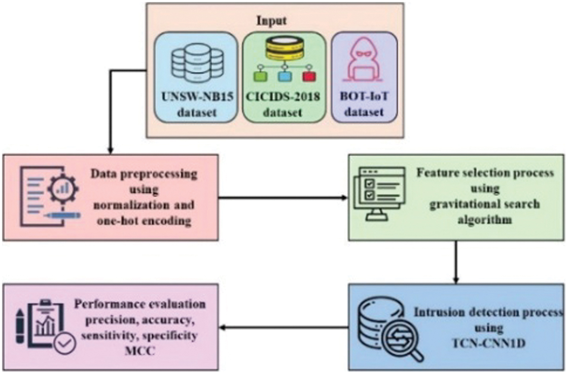Fig. 1. Workflow of the proposed CR-TCAN method in IDS.

A.DATASET DESCRIPTION

Three publicly available datasets, namely UNSW_NB15, CICIDS-2018, and Bot-IoT, are used to detect intrusion in IoT.

The UNSW_NB15 dataset [27], created by Jill Slay and Nour Moustafa at Canberra, New South Wales, and the University of Australia, is large but highly imbalanced. It contains 87.35% normal traffic, while 12.65% is abnormal, with abnormal traffic being highly uneven. Within the abnormal traffic, 5% consists of denial of service (DoS) packets, while 67% includes general packets.

The CICIDS-2018 dataset [28] contains network traffic data across eight different attacks, including benign, robot network (BOTnet), web attacks, DoS, infiltration, distributed denial of service (DDoS), brute force, and Heartbleed, totaling 15 types of traffic data. It provides system logs for each machine and network activity records. Additionally, it contains 80 features, recorded using CICFlow-Meter-V3.

The Bot-IoT dataset [29], which includes IoT traffic traces, is produced by Nickolaos Koroniotis at the universities of Canberra, Australia, and New South Wales. It is the first publicly available IoT traffic dataset. The dataset features IoT devices in a test-bed environment, including a smart refrigerator, motion-based smart lights, smart garage door, and weather station. This configuration is used for generating real-time IoT traffic for different types of attacks, such as information theft, information gathering, and DoS. The Bot-IoT dataset, stored in comma-separated values (CSV), contains 46 extracted features and 72 million records.

B.PREPROCESSING USING NORMALIZATION

Data normalization is used for data standardization and eliminates the limitations of data units by converting them into accurate, dimensionless values. Normalization is appropriate for managing multiple units and scales of indicators, which helps to balance feature weighting and prevent gradient vanishing, thereby improving the convergence rate. Min-max normalization is preferred due to its robustness and simplicity for outliers in IDS modeling. It enhances the model’s efficiency, and its formula is provided in Equation (1):

x_{ncw} = \frac{x - m i n (x)}{\max (x) - m i n (x)}

(1)

1).ONE-HOT ENCODING

Categorical data are presented in a documented form using one-hot encoding. However, this method cannot process textual data directly; therefore, it is important to convert this data into numerical formats. This technique improves data rationality during distance calculations and similarity metrics, increasing precision by converting category values into vectors. It uses sparse vectors to represent each category, avoiding numerical biases that arise from calculating distance in label encoding, as given in Equation (2):

h (x) = \frac{1}{1 + e^{- w x}}

(2)

The weight assigned to the continuous variable $w$ is balanced against the sparse vectors produced by one-host encoding to manage data rationality during similarity analysis as expressed in Equation (3):

h (x) = \frac{1}{1 + e^{- (w_{1} x_{1} + w_{2} x_{2} + \dots + w_{n} x_{n})}}

(3)

Each component represented as $x_{1}, x_{2} \dots .. x_{n}$ is associated with weight components such as $w_{1}, w_{2} \dots .. w_{n}$ based on one-hot encoding for better flow clarity. This technique transforms categorical variables into binary vectors, where a value of 1 is assigned to the index corresponding to the class and 0 elsewhere. This produces sparse representation, as shown in Equation (4):

w_{i} = [0, 0, 0, \dots, \dots, 1, 0, 0]

(4)

This method effectively manages ordinal relationships that are inadequately represented by numerical values, making it advantageous for specific categories.

C.FEATURE SELECTION USING GSA

The GSA technique is used for feature selection to select the optimal set of features that enhances the accuracy of the detection. Complex optimization problems are solved using the GSA algorithm, where each particle attracts others with their mass according to the universal law of gravitation and gravitational force. Each particle acts as an agent, representing a potential solution to the optimization problem. The different stages of the GSA are as follows.

1).Initialization

The K objects are assumed, and their positions are randomly initialized in the $i$ -th object location and $n -$ dimensional space, as defined in Equation (5):

P_{i} (t) = (P_{i}^{1}, P_{i}^{2}, \dots \dots, P_{i}^{d}, \dots \dots \dots, P_{i}^{v}); \forall i = 1, 2, \dots \dots \dots \dots . k

(5)

The position vector of an object at a specific $t$ time is called an iteration, which is represented as $P_{i} (t)$ and $P_{i}^{d}$ .

Mass Calculation:

Mass is determined by the fitness function, with each object representing a specific feature subset. The mass $W_{i} (t)$ is calculated based on the fitness value $f_{i} (t)$ at iteration $t$ , as demonstrated in Equations (6) and (7):

W_{i} (t) = \frac{f_{i} (t)}{\sum_{j = 1}^{k} f_{i} (t)}; \forall i = 1, 2, \dots, k

(6)

f_{i} (t) = \frac{{fitness}_{i} (t) - w o r s t (t)}{best (t) - w o r s t (t)}

(7)

where the fitness value is

f i t n e s s_{f} ()

i

-th object, as well as worst

(t)

and best

(t)

denotes the global extreme values at time

t

, as determined by Equations (8) and (9):

best (t) = {maximum}_{j \in {1, \dots, n}} fitness (t),

(8)

worst (t) = {minimum}_{\in {1, \dots, n}} {fitness}_{j} (t),

(9)

2).GRAVITATIONAL FORCE CALCULATION

The attractive force between two object masses is divided by the distance, which is depicted in Equation (10):

F_{i j}^{d} (t) = G (t) (\frac{W_{p i} (t) \cdot W_{0;} (t)}{D_{i j} (t) + ɛ} \cdot (P_{j}^{d} (t) - P_{i}^{d} (t)))

(10)

where the passive gravitational mass of the object at

t

time is represented by

W_{p i} (t)

, the gravitational constant is represented as

G (t)

, and the force amid mass of

t

-th is

F_{i j}^{d} (t)

, and then the

i

-th position location is

P_{i}^{d} (t)

, respectively. The decreasing coefficient of the algorithm is denoted by Equation (11):

G (t) = G_{0} * e x p (\frac{- a {* iteration}^{it}}{{iteration}_{\max}}),

(11)

The initial gravitational constant is $G_{0}$ , and the maximum number of iterations is ${iteration}_{\max}$ . The Euclidean distance between $j$ -th and $i$ -th objects is represented as $D_{i j} (t)$ , which is expressed in Equation (12):

D_{i j} (t) = {‖ P_{i} (t), P_{j} (t) ‖}_{2},

(12)

The $j$ -th dimension of the $i$ -th agent position is denoted as $r_{j}$ . The total force is calculated as a stochastic weighted sum of the forces from the $k_{best}$ objects, as shown in Equation (13):

F_{i}^{d} (t) = \sum_{j - k_{i n - 2 i + n}}^{k}, r_{j} F_{i j}^{d} (t)

(13)

The total force $F_{i}^{d} (t)$ is calculated as a randomly weighted sum of forces exerted by other agents. Thereby managing the objects, GSA significantly balances exploration and exploitation that avoids the method from getting stuck in local optima problem and improves convergence speed.

3).ACCELERATION

According to the law of motion, acceleration is calculated as provided in Equation (14):

A_{i}^{d} (t) = \frac{F_{i}^{d} (t)}{W_{i i} (t)},

(14)

where at

t

time, the mass of the

i

-th object is

W_{f f} (t)

, and the

A_{i}^{d} (t)

denotes the overall force.

4).POSITION AND VELOCITY

The position and velocity of each object are calculated using Equations (15) and (16):

V_{i}^{d} (t + 1) = A_{i}^{d} (t) + r_{i} \cdot V (t),

(15)

P_{i}^{d} (t + 1) = P_{i}^{d} (t) + V_{i}^{d} (t + 1),

(16)

The updated position of the $i$ -th objects in dimension $d$ is represented by $P_{i}^{d} (t + 1)$ , while its current state is denoted as $P_{i}^{d} (t)$ . The parameter $r_{i}$ is a stochastic variable uniformly distributed in the range [0,1].

Since GSA is used to solve continuous optimization problems, it is important to convert the GSA solutions into a binary format. The object positions are updated using Equations (17) and (18):

P_{i}^{d} (t + 1) = {\begin{matrix} 1 - P_{i}^{d} (t); & r_{i} < S f (V_{i}^{d} (t + 1)) \\ P_{i}^{d} (t); & otherwise \end{matrix},

(17)

S f (x) = \frac{1}{1 + e^{- x}}

(18)

The $d$ dimension of $i$ -th objects position is represented by $P_{i}^{d} (t)$ , $e$ is the Euler value, random value is symbolized as $r_{i}$ , and velocity is $V_{i}^{d} (t)$ of the $i$ -th agent. The binary transformation sigmoid function $S f (x)$ is used to map these continuous values into a discrete search space.

D.DETECTION USING 1D-CNN

In this section, the proposed 1D-CNN method is used for intrusion detection on one-dimensional data. Backward propagation (BP) and forward propagation (FP) are the main components of the CNN architecture. The 1D-CNN computational complexity is reduced significantly compared to 2D-CNN due to matrix operations. Shallow structures are easier to train, understand, and implement, and they effectively learn from 1D data challenges. The proposed method is suitable for training on 1D data and requires minimal computational resources, whereas training a 2D-CNN needs specialized hardware. The 1D-CNN architecture consists of pooling layer, 1D convolutional layer, dropout layers, and activation functions to process the data.

The major function of a convolutional layer is to apply filters to the input through repeated operations, creating feature maps that represent specific attributes of the data points. The weights set and input multiplications are contained within linear operations. The kernels are the results of multiplying the input by single-dimensional array weights. These unique values are obtained through operations performed during each pass, producing multiple values that form the feature map. Once the feature maps are generated, each value is passed to the rectified linear unit (ReLU) activation function that performs negative inputs to zero while leaving positive inputs unchanged, as formulated in Equation (19):

R (z) = m a x (0, z)

(19)

The activation function receives the input, which is the output of activation function $R (z)$ and $z$ , and then another CNN pooling layer is included in the convolutional layer. The model dependencies are reduced using a sub-sampling technique, and the independent information is positioned through feature mapping to address the overfitting issue. The proposed architecture’s number of parameters and computational dependencies are solved with a pooling layer that generates pooled features by considering the feature map. Based on the stride, the pooling filter size is applied, and max pooling, average pooling, and other pooling types are varied through map pooling feature selection. Max pooling captures more value in each patch, while the average value of each patch is calculated, and it is utilized to decrease the feature map dimensionality. During training, some neurons are randomly processed with inputs set to zero at a specific rate; this regularization technique helps prevent overfitting, as defined in Equation (20):

z = \frac{1}{1 - r a t e}

(20)

The noisy data training process involves more responsibilities during the training of certain nodes. However, dropout enhances the necessary scaling to select the dropout rate and network weights. The fully connected layer follows the dense layers, with an activation function and previous layers, for output mapping. Primarily, the CNN layer contains two kernel sizes with 32 filters, and ReLU is used as an activation function. Input samples are performed by this layer, which transforms the samples into (77, 32) shape vectors. Another convolutional layer, comprising 16 filters with two kernel sizes, is paired with a dropout layer set at a 0.5 rate, during training deactivating 50% of neurons to prevent overfitting. Finally, a flattering layer transforms the three-dimensional vector into a one-dimensional vector.

The feature transformation process within 1D convolutional feature extraction in the proposed architecture is expressed in Equation (21):

h_{t} = σ (W * x_{t} + b)

(21)

where

*

denotes convolution,

W

represents the kernel weights, and

b

is the bias term. This process helps extract temporal features before they are being processed by the attention mechanism.

1).PARALLEL INTERACTION ATTENTION

The proposed method effectively models both inter- and intra-model dependencies using a parallel attention structure called PIA. This module encapsulates all attack characteristics through the PIA mechanism.

i)Modality-wise local encoding via 1D convolution.Initially, a one kernel size with 1D convolution is applied to the input network sequences. This converts the original network data into a combined $d$ latent space and models the local relationships among consecutive packets, as provided in Equation (22):
$X_{s}^{'} = C o n v 1 D (X_{s}), s \in {t, a}$ (22)
The model ensures intra-model attention $(X_{t}^{'}, X_{t}^{'}, X_{t}^{'})$ to capture prosodic dynamics within the acoustic features, and cross-modal attention is $(X_{a}^{'}, X_{a}^{'}, X_{a}^{'})$ to provide interactions between textual and acoustic data.
ii)Four-way parallel threat interactionThis captures internal patterns within a single data type and the cross-correlations between them simultaneously. The four parallel attention blocks are defined in Equation (23):
$A t t e n t i o n (Q, K, V) = S o f t m a x (\frac{Q K^{⊤}}{\sqrt{d}}) V$ (23)
Intra-header attention $X_{h h}$ : Models sequence-level logic within headers to detect protocol-specific anomalies.Intra-flow attention $X_{f f}$ : Analyzes traffic flow to identify volume-based threats such as DDoS and DoS.Flow-to-header interaction $X_{f h}$ : Analyzes cross-model traffic statistics to align them with low-traffic protocol.Header-to-flow interaction $X_{h f}$ : Evaluates overall traffic behavior based on header structure. Figure 2 illustrates the architecture of the proposed PIA mechanism.
iii)Mask-aware traffic computationNetwork sessions contain varying numbers of packets; therefore, a binary mask is used to improve the model’s focus on network events while ignoring padding noise for batch processing, as defined in Equation (24):
$S_{i, j}^{(b)} = {\begin{cases} \frac{Q_{i}^{(b)} \cdot K_{j}^{(b)}}{\sqrt{d}}, & if M_{i, j}^{(b)} = 1 \\ - 10^{9}, & otherwise \end{cases}$ (24)
The softmax function helps normalize the masked scores, as presented in Equation (25):
$A^{(b)} = S o f t m a x (S^{(b)})$ (25)
This formula ensures that the attention is concentrated only on valid network traffic, thereby reducing the impact of malicious network activities.
iv)Two-stage residual enhancementAfter computation, the attention output is denoted as $\hat{A} \in R^{B \times U \times d}$ , applying two refinement stages: the first is global compression, which primarily reduces network traffic by considering convolutional blocks containing $1 \times 1$ convolutions, LeakyReLU activation, and batch normalization, as represented in Equation (26):
$A_{conv} = C o n v 2 D (M e a n (\hat{A}))$ (26)

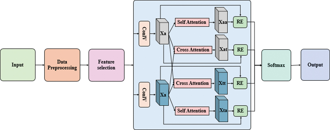Fig. 2. Architecture of the proposed method in IDS detection.

The second stage involves residual fusion with a position-wise feedforward network (FFN), which compresses the features to match the original network traffic dimensions. The position-wise FFN with broadcast backings is provided in Equations (27) and (28):

F F N (x) = W_{2} (\begin{matrix} {Dropout}_{1} \\ (G E L U (\begin{matrix} W_{1} \cdot \\ LayerNorm (x) \end{matrix})) \end{matrix})

(27)

X_{final} = Q + A_{conv} + F F N (A_{conv})

(28)

Here, the learnable weight matrices are $W_{1} \in R^{d \times d_{f f}}$ and $W_{2} \in R^{d_{f f} \times d}$ , with the model hidden dimension as $d$ and the intermediate feedforward dimension as $d_{f f}$ . Nonlinearity is introduced by the Gaussian error linear unit (GELU) function, with regularization applied through dropout.

The proposed attention-residual design is outlined along with the relevant equations. The PIA mechanism processes an $X \in R^{T \times C}$ input feature representation with temporal length $T$ and feature channels $C$ , as denoted in Equations (29), (30), and (31):

Q = X W_{Q}, K = X W_{K}, V = X W_{V}

(29)

A = \frac{Q K^{T}}{\sqrt{d}}, α = Softmax (A)

(30)

Z = α V

(31)

where the learnable projection matrices are

W_{Q}, W_{K}, W_{V}

, the embedding dimension is

d

, and the refined feature representation is obtained via residual learning, as given in Equation (32):

Y = Z + X

(32)

This helps the model to concentrate on more discriminative temporal dependencies while preserving original feature information, thus enhancing generalization and stability.

A computational analysis demonstrates the model’s suitability for IoT environments. The time complexity of the attention mechanism is expressed in Equation (33):

O (T^{2} \cdot d)

(33)

The model’s complexity is significantly reduced through a lightweight design and 1D convolutional operations; memory usage is proportional to the input size, as given in Equation (34):

O (T \cdot C)

(34)

The proposed model is feasible for resource-constrained devices due to its low computational overhead and reduced memory overhead.

The mathematical formulation of the PIA mechanism is expanded, and a channel attention mechanism variant is also included for efficiency, as shown in Equations (35), (36), and (37):

s = \frac{1}{T} \sum_{t = 1}^{T} X_{t}

(35)

α_{c} = σ (W_{2} \cdot δ (W_{1} \cdot s))

(36)

Y = X ⊙ α_{c}

(37)

where ReLU activation function is represented as

δ (\cdot)

, sigmoid function as

σ (\cdot)

, and element-wise multiplication as

⊙

, each contributing to adaptive feature calibration with reduced computational overhead.

IV.EXPERIMENTAL RESULTS AND DISCUSSION

The performance of the CR-TCAN is evaluated using the Bot-IoT, CICIDS-2018, and UNSW_NB15 datasets. The proposed CR-TCAN model is tested in a Python 3.4 environment with the following system specifications: Windows 10, 64-bit; an Intel 12th Generation i7 processor; 64 GB of RAM; and an NVIDIA GeForce RTX 3050 GPU with 8 GB of Video RAM. This setup ensures the reproducibility of the overall architecture. The CR-TCAN model performance is determined using the metrics accuracy, F1-score, recall, and precision, as defined in Equations (38)–(41). The IDS for IoT methods is assessed with these metrics.

•AccuracyThe overall performance is evaluated based on accuracy, which measures the percentage of all observations correctly predicted, including both true positives and true negatives, as defined in Equation (38):
$Accuracy = \frac{T P + T N}{T P + T N + F P + F N}$ (38)
•PrecisionThe ratio of true positives to the total number of predicted positives is demonstrated in Equation (39):
$Precision = \frac{T P}{T P + F P}$ (39)
•RecallThe ratio of actual positive samples that are accurately identified is calculated, as shown in Equation (40):
$Recall = \frac{T P}{T P + F N}$ (40)
•F1-ScoreThe F1-score combines recall and precision, which is a key metric for detection accuracy. It is calculated as a weighted average of both metrics, as defined in Equation (41):
$F 1 - S c o r e = \frac{2 P r e c i s i o n \times R e c a l l}{Precision + R e c a l l}$ (41)
where $T N$ is true negative, $F P$ is false positive, $T P$ is true positive, and $F N$ is false negative.

The proposed CR-TCAN model uses 16 and 32 filters to extract spatial features, with a 0.5 dropout rate to improve training stability and prevent overfitting. The proposed model incorporates the PIA mechanism, which utilizes $1 \times 1$ convolutions and LeakyReLU activation function to process information and packets simultaneously. It is trained over 100 epochs, employing ReLU activation in initial layers and in the latent space to model the complex IoT attack patterns. The model optimizes compression to reduce latency while maintaining maximum detection accuracy across the dataset. Table I demonstrates the hyperparameter settings for the CR-TCAN model.

Table I. Hyperparameter settings of the proposed CR-TCAN model in IDS

Model	Parameter	Settings
1D-CNN layer 1	Filters	32
	Kernel size	2
	Activation	ReLU
	Output shape	77,32
1D-CNN layer 2	Filters	16
1D-CNN layer 2	Kernel size	2
Regularization	Dropout rate	0.5
PIA mechanism	Latent space dimension	Combined latent space
	Compression	$1 \times 1$ convolutions
	Activation	LeakyReLU
	Number of epochs	100

A.CLASS-WISE PERFORMANCE VALIDATION FOR UNSW_NB15

The performance of the CR-TCAN model is evaluated by detecting high-signature threats such as worms and shellcode and distinguishing normal traffic from generic attacks with near-perfect reliability. However, it faces challenges with low-volume threats, such as backdoors and analysis, where the accuracy drops below 80%, and exploits suffer from reduced precision due to false positives. The average accuracy reflects the proposed model effectiveness across different classes. Table II demonstrates the class-wise results for the UNSW_NB15 dataset.

Table II. Class-wise results of UNSW_NB15 dataset

Class name	Precision %	Recall %	F1-score %
Analysis	79.07	79.20	79.20
Backdoor	74.66	90.77	81.93
DoS	75.74	87.60	81.24
Exploits	96.92	75.57	84.93
Fuzzers	96.85	87.10	91.72
Generic	99.95	99.54	99.74
Normal	99.97	99.97	99.97
Reconnaissance	97.49	92.56	94.96
Shellcode	100	100	100
Worms	100	100	100
AVG	92.07	91.24	91.37

B.CLASS-WISE RESULTS FOR BoT-IoT DATASET

The proposed method performs efficiently on the Bot-IoT dataset, achieving an average F1-score of 99.40%. The small variance among classes represents that the framework is highly effective in recognizing DoS, DDoS, and reconnaissance attacks with average accuracy. High precision indicates a low false alarm rate, while recall indicates the system’s effectiveness in capturing the majority of malicious activity instances. The proposed model performance on Bot-IoT is attributed to the repetitive and highly structured nature of botnet traffic patterns, which is compared with more diverse intrusion types. Table III presents the results for IDS on the Bot-IoT dataset.

Table III. Class-wise results for intrusion detection on Bot-IoT dataset

Class name	Precision %	Recall %	F1-score %
DDoS	99.91	98.83	99.36
DoS	99.01	99.19	99.09
Normal	99.10	99.86	99.47
Reconnaissance	99.55	99.96	99.55
Average (AVG)	99.23	99.58	99.40

C.CLASS-WISE RESULTS FOR CICIDS-2018 DATASET

The IDS performance using the CICIDS-2018 dataset effectively captures a wide range of modern network threats. The proposed model demonstrates high reliability with a 97.36% F1-score, indicating an efficient balance between false alarm reduction and threat detection. It is effective for pattern-heavy attacks such as DDoS-High Orbit Ion Cannon (HOOIC) and Secure Shell (SSH)-brute force, with scores exceeding 99%. Table IV represents the class-wise results for the CICIDS-2018 dataset in IDS detection.

Table IV. Class-wise results for CICIDS-2018 dataset in IDS detection

Class Name	Precision %	Recall %	F1-score %
Benign	97.87	99.82	98.84
BOT	99.75	99.54	99.64
Brute Force-Web	98.00	94.12	96.64
Brute Force-XSS	97.62	95.31	96.45
DDOS attack-HOIC	99.57	99.99	99.77
DDOS attack-LOIC-UDP	70.85	99.72	82.84
DDoS attacks-LOIC-HTTP	99.77	99.69	99.72
DoS attacks-GoldenEye	99.53	99.76	99.64
DoS attacks-Hulk	98.80	99.92	99.35
DoS attacks-SlowHTTPTest	95.14	96.34	95.73
DoS attacks-Slowloris	96.58	97.63	97.10
FTP-Bruteforce	95.63	96.32	95.97
Infilteration	98.57	94.81	96.65
SQL Injection	98.36	96.00	97.16
SSH-Bruteforce	99.98	99.92	99.94
AVG	97.33	98.10	97.36

D.PERFORMANCE ANALYSIS

This section presents both qualitative and quantitative analysis of the proposed method on CICIDS-2018, Bot-IoT, and UNSW_NB15 datasets. The CR-TCAN model performed using different metrics to enhance IDS detection performance. Table V presents the performance analysis of the IDS detection.

Table V. Performance analysis of CR-TCAN with traditional methods in IDS detection

Method	Dataset	Accuracy %	Precision %	Recall %	F1-score %
LSTM	UNSW_NB15	81.62	82.11	81.10	81.60
	CICIDS-2018	95.62	96.42	95.61	96.01
	Bot-IoT	91.71	92.64	91.71	92.17
CNN + LSTM	UNSW_NB15	85.36	81.41	85.63	83.46
	CICIDS-2018	96.43	95.78	96.52	96.14
	Bot-IoT	93.71	94.71	93.70	94.20
GRU	UNSW_NB15	83.47	82.41	83.52	82.96
	CICIDS-2018	94.85	93.68	94.86	94.26
	Bot-IoT	93.68	94.75	93.64	94.19
CNN + GRU	UNSW_NB15	82.58	84.76	83.54	84.14
	CICIDS-2018	91.82	90.89	92.36	91.61
	Bot-IoT	95.82	96.71	95.82	96.26
CR-TCAN	CICIDS-2018	98.10	97.33	98.10	97.36
	Bot-IoT	99.58	99.23	99.58	99.40
	UNSW_NB15	91.24	92.07	91.24	91.37

1).ACCURACY OVER EPOCHS FOR UNSW_NB15 DATASET

Figure 2 depicts the learning trajectory of the proposed IDS framework trained on the UNSW_NB15 dataset over 100 epochs. In the first 20 epochs, the graph shows a sharp primary learning curve, with accuracy increasing from 60% to 85%, eventually stabilizing at a maximum of 92%. The consistency between training and validation accuracies indicates the model’s quality, as it generalizes well and avoids overfitting the training data. The UNSW_NB15 dataset is known for its modern attack signatures, complexity, and high noise levels. The consistent performance across both sets demonstrates that the proposed method is reliable for distinguishing between sophisticated exploits and normal network traffic. Figure 3 demonstrates the performance analysis of UNSW_NB15 dataset accuracy over epochs for IDS.

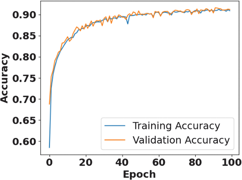Fig. 3. Performance analysis of UNSW_NB15 dataset accuracy over epochs for IDS.

2).LOSS VERSUS ACCURACY FOR THE UNSW_NB15 DATASET

Figure 3 presents the error rate of the proposed model over 100 epochs using the UNSW_NB15 dataset. The validation loss starts at 0.8, and the training loss starts at 1.2, with both values decreasing before 20 epochs. Both lines converge to a low value of approximately 0.2 at 100 epochs. Throughout the process, the training and validation losses remain close to each other. The proposed model does not overfit, indicating its ability to generalize effectively and manage less classification error between normal and malicious traffic. Figure 4 illustrates the performance analysis of loss against accuracy in the IDS using the UNSW_NB15 dataset.

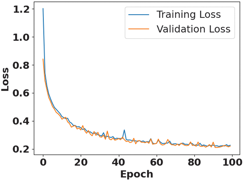Fig. 4. Loss versus accuracy performance analysis using UNSW_NB15 dataset in IDS.

3).CONFUSION MATRIX FOR THE UNSW_NB15 DATASET

The proposed model represents multi-class classification performance. Classes such as normal, worms, generic, and shellcode have higher values, each achieving 7,418 accurate predictions with 100% accuracy. Inter-class confusion occurs between backdoor and analysis, with over 1,000 instances of analysis misclassified as backdoor. Exploits and DoS have leakage classes, where 833 exploits are incorrectly labeled as DoS. During processing, identical sample counts across several classes are balanced. The proposed model effectively distinguishes between malicious and normal traffic, although it struggles to classify attack types with overlapping feature signatures such as backdoor, analysis, and exploits. Figure 5 represents the UNSW_NB15 dataset confusion matrix.

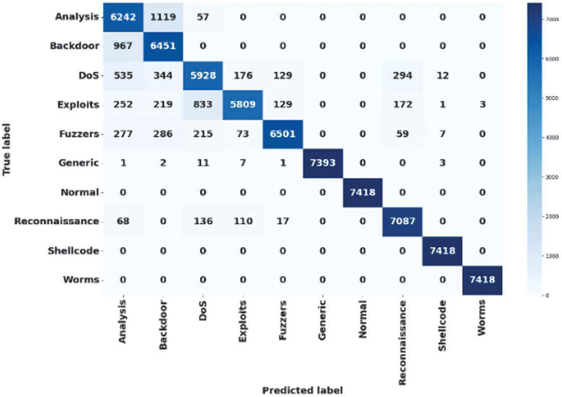Fig. 5. Confusion matrix performance analysis using UNSW_NB15 dataset.

4).ROC CURVE FOR THE UNSW_NB15 DATASET

The CR-TCAN model differentiates traffic classes within the UNSW_NB15 dataset. This graph plots true positive rate (TPR) against false positive rate (FPR) for each category. The overall classification quality is measured by area under the curve (AUC) values, which are 1.0000 for normal, generic, worms, and shellcode, indicating perfect separation of these classes. The proposed model maintains a low false alarm rate across all attack types while achieving a high detection rate. Figure 6 displays the ROC curve for the proposed model on the UNSW_NB15 dataset.

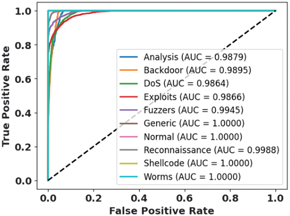Fig. 6. ROC curve for the proposed method using the UNSW_NB15 dataset in IDS detection.

5).ACCURACY VERSUS LOSS FOR THE Bot-IoT DATASET

Figure 7 demonstrates the accuracy over epochs, evaluated during model training on the Bot-IoT dataset, indicating an efficient learning process. Both training and validation accuracies, which range between 50% and 60%, increase rapidly around 60 epochs. The Bot-IoT dataset is complex and helps to identify multiple network attacks, demonstrating that the method effectively differentiates botnet traffic features and classifies them with high precision on unseen data.

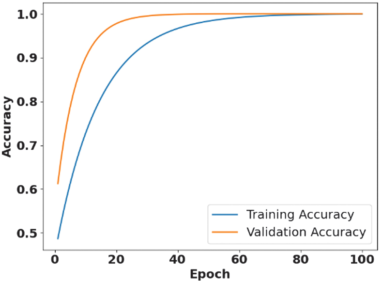Fig. 7. Performance analysis of accuracy against epochs in intrusion detection.

6).LOSS VERSUS EPOCHS FOR THE Bot-IoT Dataset

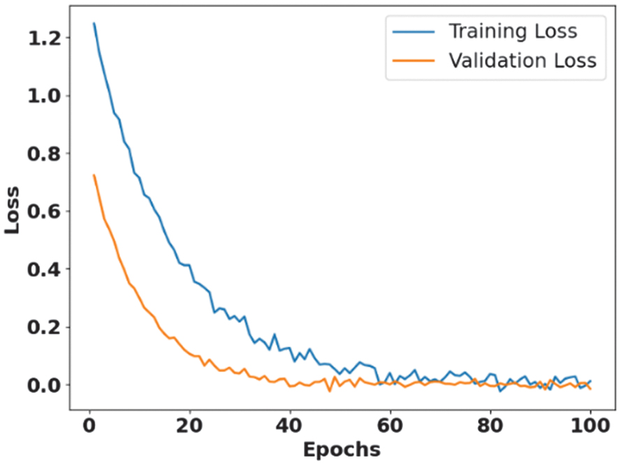
Figure 8 illustrates the loss over epochs for the Bot-IoT dataset. The proposed method’s loss decreases as it trains over 100 rounds on both training and testing data. The model reaches nearly zero loss at approximately 60 epochs, indicating improved learning efficiency and better convergence.

Fig. 8. Loss versus epochs in IDS detection.

7).CONFUSION MATRIX FOR THE Bot-IoT DATASET

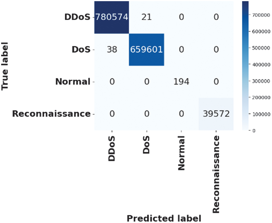
Figure 9 illustrates the Bot-IoT dataset confusion matrix, showing that the proposed framework achieves high classification performance across classes such as normal, DoS, DDoS, and reconnaissance. Initially, TPs represent correct predictions of actual labels. The model attains 100% accuracy for 194 normal instances and 39,572 reconnaissance instances, respectively.

Fig. 9. Bot-IoT dataset confusion matrix for IDS detection.

8).ROC CURVE FOR Bot-IoT DATASET

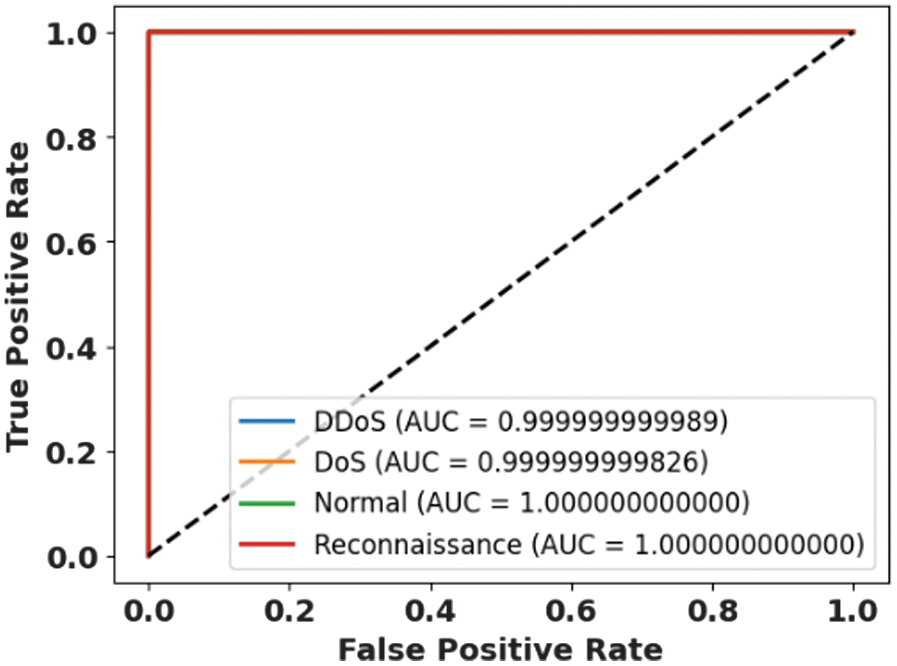
In Fig. 10, the proposed approach distinguishes between cyberattacks and normal traffic, including reconnaissance and DDoS attacks. The TPR is plotted against FPR to achieve an AUC value of 1.0. The proposed model effectively identifies malicious patterns amidst high-volume IoT traffic, ensuring maximum reliability for real-time security applications.

Fig. 10. CICIDS-2018 dataset ROC curve for IDS detection.

9).ACCURACY VERSUS EPOCHS FOR CICIDS-2018

In Fig. 11, the proposed model represents its learning capability across training and validation accuracy, achieving 98% within the initial 20 epochs. This graph also addresses overfitting issues by efficiently managing unseen network traffic. The 98.10% accuracy indicates its effectiveness in detecting complex intrusions in large-scale environments.

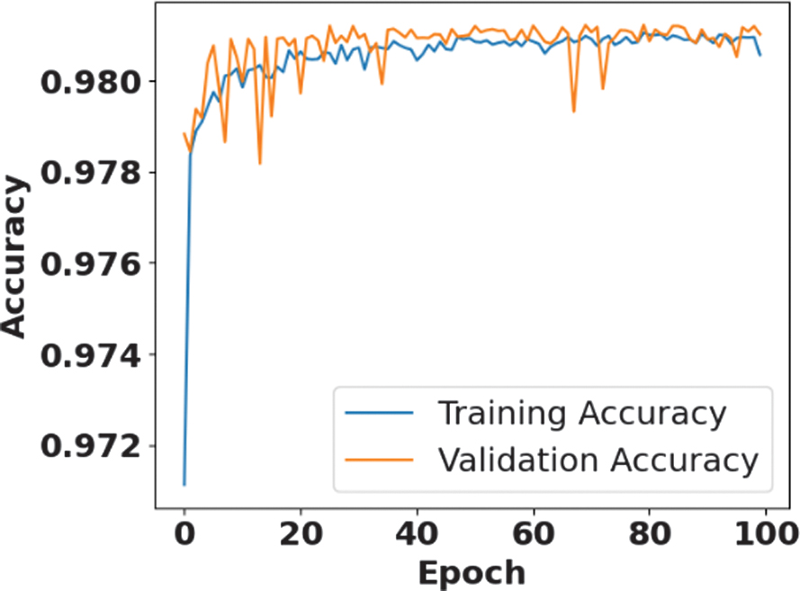Fig. 11. Accuracy versus loss for IDS detection using CICIDS-2018 dataset.

10).LOSS VERSUS EPOCHS FOR CICIDS-2018 DATASET

Figure 12 illustrates the loss curve for the CICIDS-2018 dataset. Both training and validation losses decrease and stabilize within the first 20 epochs. The primary drops indicate the model quickly learns the key features of initial intrusion data. It then stabilizes at minimal loss values around 0.075. The proposed model maintains prediction performance over 100 epochs by avoiding overfitting and improving generalization.

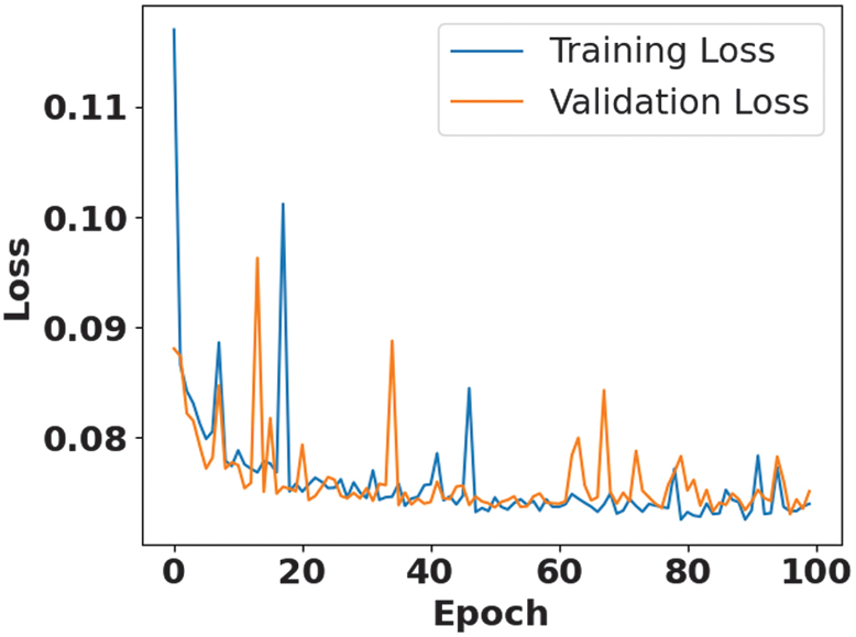Fig. 12. Loss versus epochs in IDS detection using CICIDS-2018 dataset.

11).CONFUSION MATRIX FOR CICIDS-2018 DATASET

Figure 13 displays the classification performance across different network traffic classes. The majority classes, including benign traffic and DoS attacks, are correctly identified with high precision. The proposed model effectively differentiates between threats across various categories. The confusion matrix highlights the model’s reliability in classifying complex and diverse intrusions in a multi-class environment.

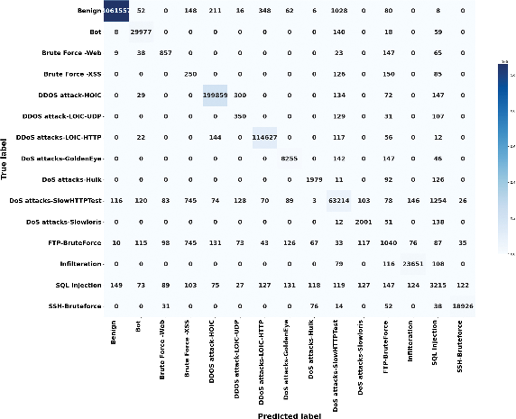Fig. 13. Confusion matrix of the CICIDS-2018 dataset for IDS detection.

E.ABLATION STUDY

The proposed approach is compared with baseline models to enhance the overall performance of the IDS. The performance of the proposed model on these three datasets is compared with traditional models to demonstrate its effectiveness and superiority. This efficiency improves the model’s generalization, thereby reducing overfitting. The combination of the TCN layer, 1D CNN, and dense softmax is crucial for optimal performance. The TCN layer effectively captures long-term temporal patterns in network traffic, enabling the model to identify complex attack sequences that traditional recurrent neural networks (RNNs) fail to do. Table VI presents an ablation study comparing the proposed method with existing techniques.

Table VI. Ablation study for the proposed method with traditional approaches using three datasets

Method	Dataset	Accuracy %	Precision %	Recall %	F1-score %
1D-CNN + Dense (Softmax)	UNSW_NB15	80.36	81.25	80.88	81.06
	CICIDS-2018	95.82	94.58	95.77	95.17
	Bot-IoT	97.52	96.51	97.58	97.04
TCN + Dense (Softmax) 1D-CNN + TCN (without Softmax optimization)	UNSW_NB15	85.62	84.55	85.69	85.11
	CICIDS-2018	92.58	91.57	92.55	92.05
	Bot-IoT	96.32	95.55	96.27	95.90
Baseline Deep Neural Network (DNN)	UNSW_NB15	84.62	85.51	86.21	85.85
	CICIDS-2018	90.58	92.36	91.54	91.94
	Bot-IoT	95.36	94.87	95.66	95.26
Bi-LSTM + Dense (Softmax)	UNSW_NB15	81.85	82.65	81.54	82.09
	CICIDS-2018	97.85	96.36	97.84	97.09
	Bot-IoT	96.42	96.33	95.55	95.93
CR-TCAN	CICIDS-2018	98.10	97.33	98.10	97.36
	Bot-IoT	99.58	99.23	99.58	99.40
	UNSW_NB15	91.24	92.07	91.24	91.37

F.STATISTICAL AND COMPUTATIONAL ANALYSIS:

In IDS, statistical and computational analyses show that the model performs efficiently, indicating its suitability for real-time network monitoring. This analysis emphasizes computational overhead, where inference and training times are critical for the system’s ability to detect new threats. The proposed model significantly outperforms other models, reducing inference latency to 0.2482, which is essential for preventing breaches. Table VII presents the computational and statistical analysis of the proposed model.

Table VII. Computational and statistical analysis of the proposed method

Dataset	Method classifier name	Training time (s)	P-value	Inference time (s)	Memory usage	FLOPS	Parameters
UNSW_NB15	LSTM	158.36	1.5872	8.4771	5823.25	32.14	1,471,446
	CNN + LSTM	179.32	3.4122	10.5823	8555.25	35.84	1,471,446
	GRU	162.82	2.8525	9.7412	7456.24	39.41	1,471,446
	CNN + GRU	182.52	3.8523	9.9987	8523.71	40.54	1,471,446
	CR-TCAN	129.781	0.6170	2.6423	3368.45	25.12	1,471,446
CICIDS-2018	LSTM	505.21	1.7852	63.14	4521.14	45.84	1,082,243
	CNN + LSTM	511.47	3.1236	65.47	4836.21	51.24	1,082,243
	GRU	523.14	4.2541	68.25	5521.14	55.25	1,082,243
	CNN + GRU	553.14	4.3541	70.54	6014.25	61.24	1,082,243
	CR-TCAN	420.38	0.4365	55.36	2562.14	34.14	1,082,243
Bot-IoT	LSTM	634.53	1.2563	105.58	21478.25	52.31	142,148
	CNN + LSTM	710.58	1.2589	106.58	25414.87	58.14	142,148
	GRU	650.83	2.3684	114.85	28563.14	62.31	142,148
	CNN + GRU	701.85	2.0147	108.25	25874.12	65.84	142,148
	CR-TCAN	520.56	0.2482	94.15	20911.39	42.21	142,148

G.K-FOLD VALIDATION

Various existing approaches are tested across different K-fold configurations (2, 3, 5, and 7) using three major datasets. The proposed method performs more efficiently than traditional approaches such as GRU and LSTM, achieving 99.58% accuracy on the Bot-IoT dataset. The proposed approach balances training and testing on these specific network traffic patterns, while UNSW_NB15 dataset remains challenging for classification. The proposed framework improves recall and precision, thereby reducing the risk of missed detections compared with existing approaches. Table VIII depicts K-fold validation results for various numbers of folds, compared with traditional approaches.

Table VIII. K-fold validation for the proposed framework is compared with traditional approaches

Method	Fold	Dataset	Accuracy (%)	Precision (%)	Recall (%)	F1-score (%)
LSTM	2	UNSW_NB15	80.62	81.42	80.25	80.83
	3		78.61	79.42	78.66	79.03
	5		81.62	82.11	81.10	81.60
	7		77.85	78.71	77.61	78.15
	2	CICIDS-2018	90.52	91.55	90.17	90.85
	3		92.66	91.58	92.45	92.01
	5		95.62	96.42	95.61	96.01
	7		94.89	93.58	94.58	94.07
	2	Bot-IoT	89.71	88.52	89.71	89.11
	3		88.93	87.14	88.96	88.04
	5		91.71	92.64	91.71	92.17
	7		86.21	85.69	86.21	85.94
CNN + LSTM	2	UNSW_NB15	83.23	84.51	83.41	83.95
	3		80.52	81.82	80.74	81.27
	5		85.36	81.41	85.63	83.46
	7		82.47	83.66	82.47	83.06
	2	CICIDS-2018	91.58	92.55	91.47	92.00
	3		94.36	94.25	94.21	94.22
	5		96.43	95.78	96.52	96.14
	7		93.54	93.66	92.56	93.10
	2	Bot-IoT	92.36	91.78	92.36	92.06
	3		90.82	91.75	90.82	91.28
	5		93.71	94.71	93.70	94.20
	7		91.74	92.58	91.75	92.16
GRU	2	UNSW_NB15	78.63	79.62	78.41	79.01
	3		81.54	82.01	81.64	81.82
	5		83.47	82.41	83.52	82.96
	7		79.65	80.47	79.64	80.05
	2	CICIDS-2018	92.66	91.52	92.54	92.02
	3		90.25	90.86	90.67	90.76
	5		94.85	93.68	94.86	94.26
	7		92.36	91.58	92.36	91.96
	2	Bot-IoT	90.82	91.72	90.82	91.26
	3		91.78	92.83	91.78	92.30
	5		93.68	94.75	93.64	94.19
	7		92.58	93.71	92.55	93.12
CNN + GRU	2	UNSW_NB15	78.63	79.51	77.81	78.65
	3		80.88	81.54	80.64	81.07
	5		82.58	84.76	83.54	84.14
	7		79.63	80.57	79.55	80.05
	2	CICIDS-2018	89.62	88.52	89.21	88.86
	3		88.62	88.45	88.21	88.32
	5		91.82	90.89	92.36	91.61
	7		90.54	89.85	90.01	89.32
	2	Bot-IoT	92.81	93.58	92.81	93.19
	3		93.58	94.78	93.58	94.17
	5		95.82	96.71	95.82	96.26
	7		92.36	93.52	92.51	93.01
CR-TCAN	2	UNSW_NB15	89.14	88.36	89.63	88.90
	3		90.36	89.64	90.71	90.17
	5		91.24	92.07	91.24	91.37
	7		88.64	89.41	88.14	88.77
	2	CICIDS-2018	96.36	95.22	96.52	95.86
	3		94.58	95.66	94.89	95.27
	5		98.10	97.33	98.10	97.36
	7		95.55	94.86	95.66	95.25
	2	Bot-IoT	97.84	97.85	97.84	97.84
	3		95.77	96.55	95.88	96.21
	5		99.58	99.23	99.58	99.40
	7		96.88	97.82	96.88	97.34

H.COMPARATIVE ANALYSIS

Table IX compares the proposed CR-TCAN with 1D-CNN [21], CNN + GRU [22], CTGAN [23], CNN + LSTM [24], and Botnet Detection based on an Ensemble Feature Selection with a Hybrid DL model in IDS (BOT-EnsIDS) [25] on Bot-IoT, CICIDS 2018, and UNSW_NB15 datasets. The CR-TCAN achieves accuracies of 98.10% on CICIDS-2018, 99.58% on Bot-IoT, and 91.24% on UNSW_NB15 datasets.

Table IX. Comparative analysis of the proposed CR-TCAN across UNSW_NB15, CICIDS 2018, and Bot-IoT datasets

Method	Dataset	Accuracy %	Precision %	Recall %	F1-score %
1D-CNN [21]	UNSW_NB15	80.65	82.66	80.65	81.15
CNN + GRU [22]	CICIDS-2018	97.95	NA	NA	NA
CTGAN [23]	CICIDS-2018	0.93	0.87	0.81	0.81
CNN + LSTM [24]	UNSW_NB15	78.36	NA	NA	NA
BOT-EnsIDS [25]	Bot-IoT	97.00	97.50	97.50	97.50
CR-TCAN	CICIDS-2018	98.10	97.33	98.10	97.36
	Bot-IoT	99.58	99.23	99.58	99.40
	UNSW_NB15	91.24	92.07	91.24	91.37

I.DISCUSSION

This section discusses the use of the proposed CT-TCAN method to detect malicious activity in IoT, thereby improving detection accuracy. Traditional approaches such as 1D-CNN, CNN + GRU, and CTGAN struggle with noisy, imbalanced training data, leading to inefficient performance and lower detection rates. Synthetic data generated by traditional GANs fail to capture diverse activities, especially if the GAN is not properly trained, leading to overfitting. Additionally, the existing attention mechanism is prone to learning normal behaviors, resulting in a high FP rate. The Bot-IoT, UNSW_NB15, and CICIDS-2018 datasets are used to evaluate the model’s performance. The GSA method is employed for feature selection to address the maximum relevant attributes and enhance detection accuracy. The proposed CR-TCAN method achieves accuracies of 99.58% for Bot-IoT, 91.24% for UNSW_NB15, and 98.10% for CICIDS-2018.

V.CONCLUSION

This research employed the proposed CR-TCAN method to detect anomalies and malicious network traffic activities in IoT. The approach improved the IDS’s performance by selecting crucial features, thereby increasing the detection rate. The CICIDS 2018, Bot-IoT, and UNSW_NB15 datasets were used for training and testing, leading to enhanced detection performance. During preprocessing, one-hot encoding and min-max normalization were applied to transform the original data into categorical data, and GSA was used to select important features, further boosting detection accuracy. The CR-TCAN method achieved 99.58% accuracy on Bot-IoT, 91.24% on UNSW_NB15, and 98.10% on CICIDS-2018. Future work of this research will integrate the proposed method with self-supervised learning to identify emerging zero-day threats from unlabeled network traffic, reducing reliance on manual data tagging. Additionally, this method will help improve the security of information systems by accurately detecting malicious activities.

Intrusion Detection System in IoT Using Convolutional Residual Temporal Cross-Attention Network