JAIT

I.INTRODUCTION

Machine learning (ML) is one of the subfields of artificial intelligence (AI). Ref. [1] allows computers to explore ways to improve problem-solving efficiency based on experience [2,3]. Deep learning (DL) is a research direction in the field of ML [4,5]. Based on the learning method of the model, ML can be broadly classified into supervised, unsupervised, and semisupervised learning [6]. Clustering analysis is one of the unsupervised learning methods [7]. In cluster analysis, for a large amount of data or samples, the computer tries to find the classification rules based on the characteristics of the data. It follows this classification rule to classify the data reasonably. After several iterations, finally, similar data are classified into one group.

Cluster analysis applies to many different fields. Fahad, S. et al. (2023) [8] used cluster analysis to predict rainfall. Dreyer, J. et al. (2022) [9] looked for the common features and differences in the care that people with dementia currently receive in order to design the care that different levels of patients need. Azzi, D. V. et al. (2022) [10] used cluster analysis to determine students’ quality of life by combining multiple factors to help teachers guide students in finding response strategies. Negi, S. S. et al. (2022) [11] used clustering and network analysis of over one million SARS-CoV-2 spike protein sequences to help doctors design vaccines for multiple local strains. Naciti, V. et al. (2022) [12] analyzed a large amount of literature on corporate governance and sustainability, finding trends recent in scholarly research in this area. In addition to the applications of cluster analysis in the above fields, it can also be used in agriculture [13], Internet-of-Things [14], and investment [15].

In recent years, numerous researchers have attempted to introduce new clustering algorithms from diverse angles to improve optimization. Liang, B. et al. (2022) [16] simulated the process of cell division and merging in living organisms and developed a novel two-stage algorithm for clustering cell groups. This algorithm involves a continuous validation and correction mechanism. This algorithm’s advantage was that it applies to many dataset types, including imbalanced datasets and spherical nonspherical clusters. The paper [17] proposed a novel clustering algorithm. It started with a fast mean-shift algorithm to locate the center of the data distribution quickly. Next, the parameters in the algorithm were adjusted by calculating the distance distribution between the centroids and the other points. The process of this new clustering algorithm was similar to the radar scan. The aim is to classify a cluster efficiently and accurately.

The paper [18] presented the TPLMM-k algorithm, which pioneered the use of the asymmetric distribution of the k-means algorithm to recognize the existence of bacteria on digital images. Compared to the gaussian mixture model (GMM) method, which is currently used more frequently, better image decomposition metrics can be obtained using this novel method. The paper [19] proposed a metaheuristic clustering task algorithm based on water wave optimization (WWO). The original WWO method may have problems of missing optimal information and premature convergence. The improved method uses the updated search mechanism and the decay operator to solve these two problems separately.

The paper [20] wanted to classify customer types dynamically. The innovative framework presented in the study utilizes a time series of recency, frequency, and monetary variables to represent each customer’s behavior. Experimental results showed that finding a suitable model for target customer groups in different industries is feasible. The framework proposed in the paper [21] consisted of kernel fuzzy C-means clustering (KFCM) and a teaching learning-based optimization algorithm (TLBO). The strength was that it improved clustering compactness. Using the same dataset, the optimized clustering algorithm performs better than the genetic algorithm and the particle swarm algorithm for the model. The paper [22] developed a recommendation system for recommending content from users with similar hobbies to the new users. The hybrid sparrow clustered (HSC) system consists of two phases: training and recommendation. Clustering analysis was mainly used in the first phase to classify clusters based on a rating matrix generated from the data.

The paper [23] introduced the firefly algorithm (FA) to find the maximal point of the variance ratio criterion (VRC), which is the fitness function in this study. Wang, S. (2016) [24] proposed chaotic biogeography-based optimization (CBBO) and applied it to centroid-based clustering methods. Chandirasekaran, D. et al. (2019) [25] applied the cat swarm algorithm (CSA) to minimize the intra-cluster distances between the cluster members. The CSA method can be transferred to cluster analysis and bankruptcy prediction [26].

In the following part, Section II reviews related works and some classical clustering algorithms. Section III introduces the encoding strategy used and the criteria function. Section IV describes the PSO and chaotic particle swarm optimization (CPSO) algorithms. Section V contains simulation data and results of this algorithm compared with other optimization algorithms through VRC values. Finally, Section VI summarizes our work and suggests possible future directions for the improvement of this work.

II.RELATED WORK

Before cluster analysis, the data outliers from the dataset need to be removed, reducing interference of invalid samples to the cluster analysis results. Cluster analysis is a way of exploring the characteristics and rules that exist in the data instead of relying on experience gained before. The classification will follow these characteristics and rules to achieve a reasonable result.

Cluster analysis does not only classify by one particular characteristic. Considering multiple characteristics is necessary to obtain comprehensive and accurate classification results. The cluster analysis results may output different conclusions depending on the cluster method used. The number of final clusters obtained from cluster analysis may differ from researcher to researcher, even based on the same dataset.

Some people have focused on optimization algorithms for clustering analysis. In the paper [27], a new density peak clustering algorithm (NDPC) is proposed. It was built based on a combination of cosine similarity and exponential decay function. With the enhance by an improved Harris hawks optimization algorithm (FHHO), the FHHO-NDPC algorithm has significant advantages in terms of convergence speed and solution precision when solving high-dimensional problems. A adaptive semisupervised clustering (A-SSC) algorithm was introduced in the paper [28]. This model was a combination of the nonsmooth optimization method and an incremental approach without the requirements of subgradient evaluations. By observing the circulation and convergence of water in the hydrologic cycle process, hydrologic cycle optimization (HCO) was proposed [29]. The HCO was abstracted into a simplified model. Tests were performed to evaluate the optimization effectiveness of the HCO algorithm. In this paper [30], the authors used a combination of the whale optimization algorithm and tabu search (WOATS) for data clustering. Regardless of the dataset’s size, WOATS was able to efficiently identify high-quality centers in a limited number of iterations. The effectiveness of WOATS was demonstrated by the significant differences observed in different outlier criteria. Fig. 1 shows the classification of clustering analysis and features are listed in Table I.

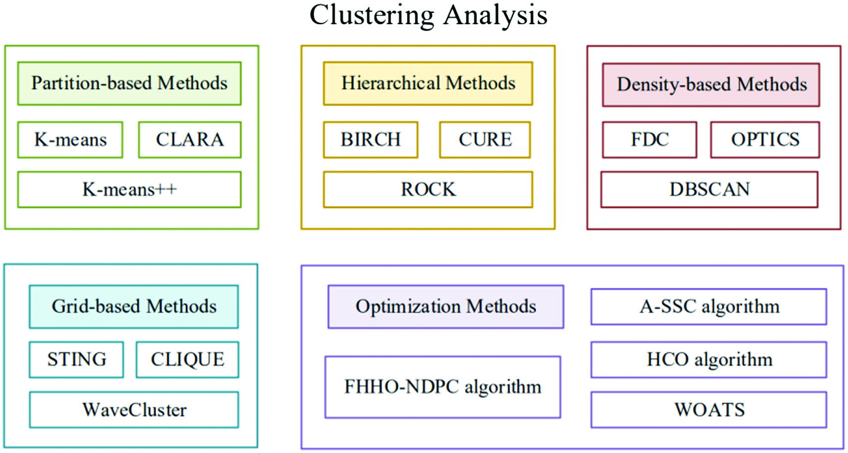Fig. 1. Classification of clustering analysis.

Table I. Methods of clustering analysis

Type	Name	Feature
Partition-based methods	K-means [37]	Using the center of a cluster to represent a cluster
	K-means++ [38]	Improvements have been made in the way K-means performs the initialization of cluster centers
	CLARA [39]	Sampling techniques are used to enable the processing of large-scale data
Hierarchical methods	BIRCH [40]	Using a tree structure to process the dataset
	CURE [41]	Partitioning the dataset by randomly selected samples and global clustering after local clustering of each partition
	ROCK [42]	Taking the influence of surrounding objects into account when calculating the similarity of two objects
Density-based methods	DBSCAN [43]	Using spatial indexing techniques to search the neighborhood of an object, introducing the concept of density reachability
	OPTICS [44]	Different parameters can be set for different clusters
	FDC [45]	Dividing the entire data space into rectangular spaces
Grid-based methods	STING [46]	Using grid cells to preserve data statistics, thus enabling multi-resolution clustering
	Wave Cluster [47]	Introducing the wavelet transform, mainly used in signal processing
	CLIQUE [48]	Combining grid and density clustering algorithms
Others	Quantum Clustering [49]	Introducing the theory of quantum potential energy from quantum mechanics
	Kernel Clustering [50]	Mapping of kernel functions to highlight features not originally shown
	Spectral Clustering [51]	Clustering on arbitrarily shaped sample spaces and convergence to a globally optimal solution
Optimization methods	FHHO-NDPC algorithm [27]	Significant improvements in convergence speed and solution accuracy when solving high-dimensional problems
	A-SSC Algorithm [28]	Better than the other four algorithms in identifying compact and well-separated clusters
	HCO algorithm [29]	Abstracted from the hydrological cycling phenomenon
	WOATS [30]	Significant differences can be observed in different outlier criteria

III.METHODOLOGY

A. SEARCH SPACE: ENCODING STRATEGY

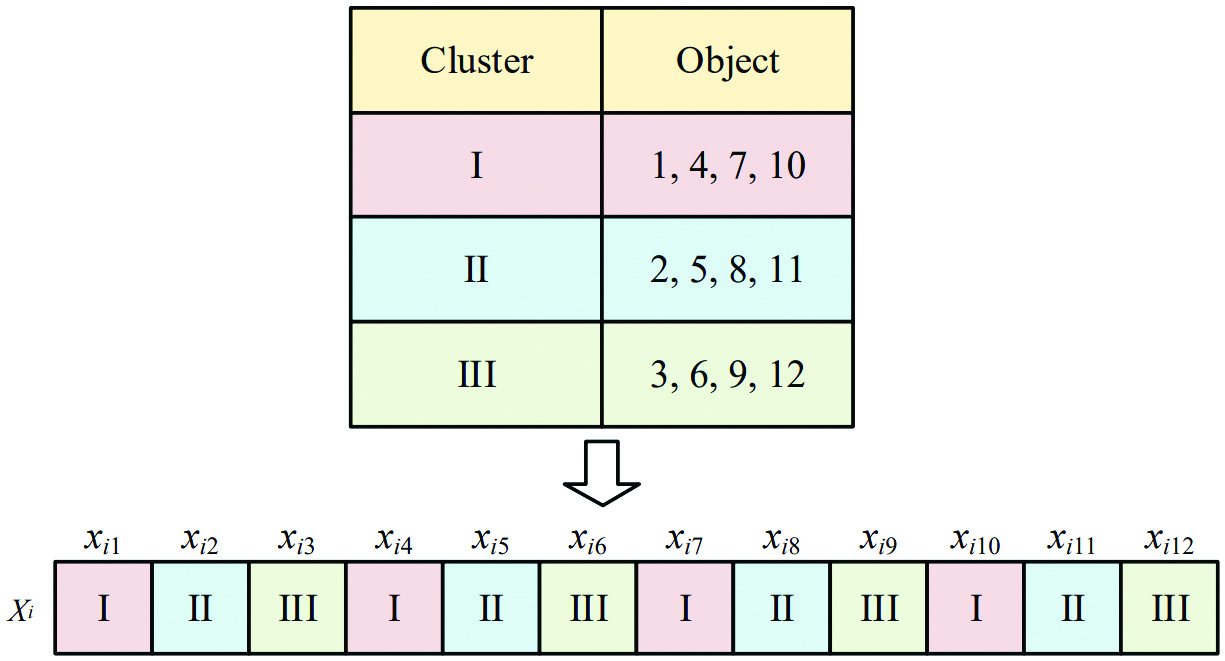
The dimension $n$ of the search space is equal to the number of objects to be clustered and analyzed. $k$ denotes the number of clusters hoped to be classified. j denotes the jth object. i denotes the ith individual. In the figure, $X_{i} = {X_{i 1}, X_{i 2}, X_{i 3} \dots X_{i j}}, j \in [1, 12]$ . The number of target clusters is $k = 3$ . The first cluster contains the 1^st, 4^th, 7^th, and 10^th object. The second cluster contains the 2^nd, 5^th, 8^th, and 11^th object. The third cluster contains the 3^rd, 6^th, 9^th, and 12^th object. Fig. 2 shows the representation of encoding.

Fig. 2. The representation of encoding.

B.CRITERION FUNCTION

The VRC is a statistical test to determine the optimal number of clusters to a dataset. VRC measures the ratio of between-cluster variance to within-cluster variance. If the ratio is high, the data should be divided into more clusters; if the ratio is low, the data can be well represented by fewer clusters. The VRC requires balancing the separation between groups and the similarity within classes. VRC is a simple and effective method for determining the optimal number of clusters in a dataset. Therefore, the VRC is defined in equation, as follows:

{VRC}_{k} = \frac{tr (S_{B})}{tr (S_{W})} \times \frac{(N - k)}{(k - 1)},

(1)

where

k

denotes the number of clusters,

N

denotes the number of objects in the dataset,

B

represents the between-group sum-of-squares cross-products matrix, and

W

represents the within-group sum-of-squares cross-products matrix.

S_{W}

denotes the average of the within-class scatter matrix,

S_{B}

denotes the between-class scatter matrix, and

tr ()

denotes the trace of the scattering matrices.

IV.OPTIMIZATION METHOD

In many algorithms, scholars often pay attention to the variation of the loss function. There is no doubt that we want the loss function to be as small as possible. Thus, it is necessary to use optimization methods. Commonly used optimization algorithms can be broadly classified into two categories, exact algorithms, and heuristics algorithms. Figure 3 shows the categorization of optimization algorithms.

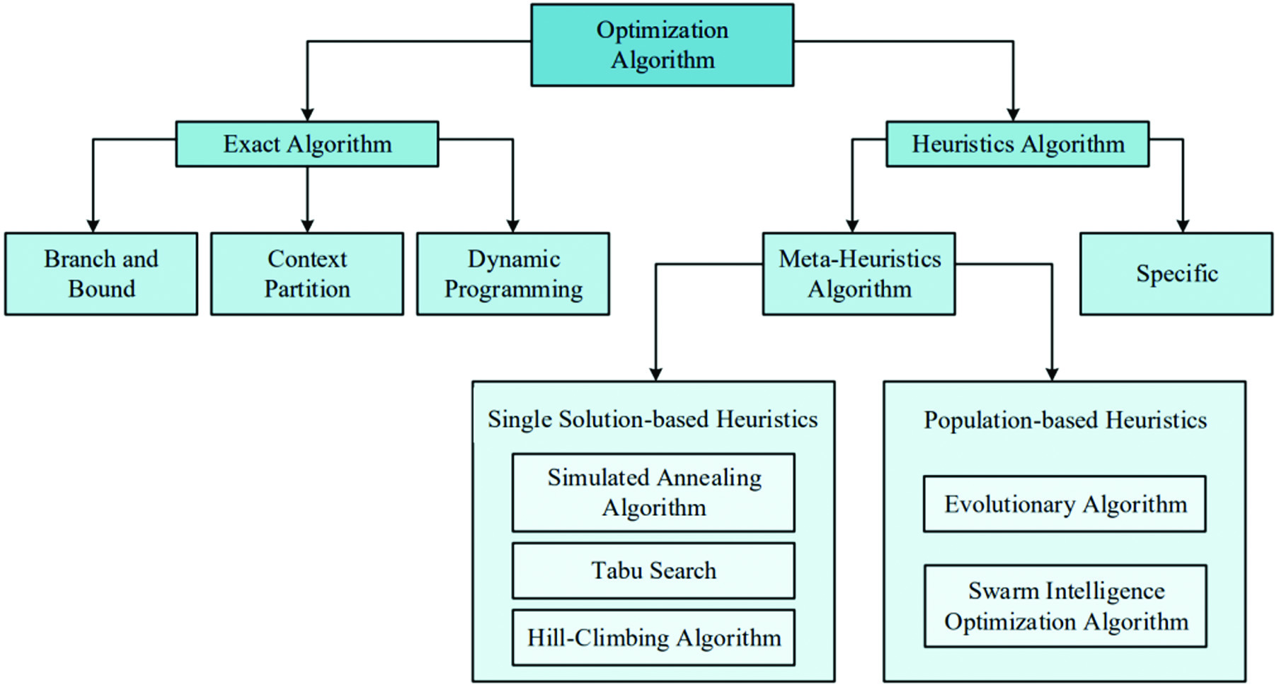Fig. 3. Classification of optimization algorithms.

Swarm intelligence optimization algorithms are inspired by the behaviors of birds flocking, ants searching for food, and bees searching for flowers. The optimization efficiency is improved by simulating the movement and information exchange of a large number of particles [31,32]. This method uses the knowledge and experience of each individual in the group to make collective decisions and realizes the search for the optimal solution through cooperation and collaboration within the group. This method is usually used for optimizing complex functions, such as finding the maximum or minimum value of a function [33] or combinatorial optimization [34].

A.PARTICLE SWARM OPTIMIZATION

The particle swarm optimization (PSO) algorithm is a commonly used algorithm in swarm intelligence optimization. The social behavior of birds inspires it in groups. The algorithm uses multiple particles to track the position of the best particle and the best position of itself that has been obtained so far.

Initially, the particles start from a random position and continuously transmit information to locate the optimal solution. In each information transfer, the particle updates the optimum solution it found and learns the optimum solution found by the whole group. The optimal solution discovered by a particle alone is referred to as the individual extremum, while the optimal solution currently found by the entire group is known as the global extreme. Through continuous iterations, the activities of the whole group in the space become continuously ordered to obtain the optimal solution eventually.

The PSO algorithm starts from a random solution and evaluates the quality of the solution through fitness during the iterative process. Compared with classical genetic algorithms, PSO is simpler to implement as there is no possibility of variation. The flow of the algorithm for finding the extremum according to the particle swarm algorithm function is shown in Fig. 4.

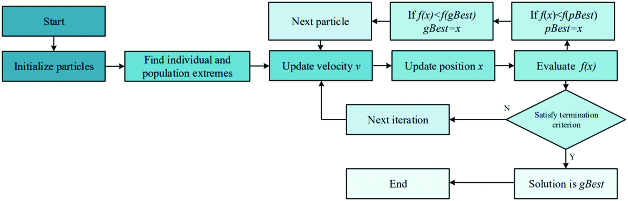Fig. 4. The flow of the PSO algorithm.

The formulas in the key steps of the PSO algorithm are the velocity vector iteration formula and the position vector iteration formula for particle $i$ :

v_{i} = ω v_{i} + c_{1} r_{1} (p {Best}_{i} - x_{i}) + c_{2} r_{2} (g Best - x_{i})

(2)

x_{i} = x_{i} + v_{i}

(3)

Equation (2) is the iterative formula for the velocity vector $v_{i}$ . Equation (3) is the iterative formula for the position $x_{i}$ . The parameter $ω$ is called the inertia weight, which takes values in the interval [0,1]. The parameters $c_{1}$ and $c_{2}$ are learning factors. $r_{1}$ and $r_{2}$ are random probability values between [0,1]. $p {Best}_{i}$ represents the historical best position vector of particle $i$ and the population’s historical best position vector. $g Best$ represents the population’s historical best position vector.

B.CHAOTIC PSO

In the chaos, even the smallest gaps that appear at the beginning can be infinitely magnified, leading to processes that cannot be predicted with different outcomes. Although chaos and randomness can make events unpredictable, the reasons are different. Chaos has no randomness. Randomness means that even the exact same initial conditions will measure different outcomes. The result is independent of the initial conditions.

Chaos leads to different results because of the extreme sensitivity of the results to the initial conditions. Chaotic optimization algorithms achieve global optima according to their laws of motion. It is easy to get rid of local optima and have better global optimization performance, which can compensate for the original PSO algorithm’s tendency to fall into local extremes and slow convergence at a later stage. Figure 5 shows the flowchart of chaotic PSO. Logistic mapping is a typical chaotic system, and the mapping relationship is as follows:

z_{i + 1} = μ z_{i} (1 - z_{i}), z_{i} \in (0, 1],

(4)

where μ is the control variable. After the value of

μ

is determined, a deterministic time series

z_{1}, z_{2}, z_{3} \dots

can be iterated from any initial value

z \in [0, 1]

i

represents the number of iterations.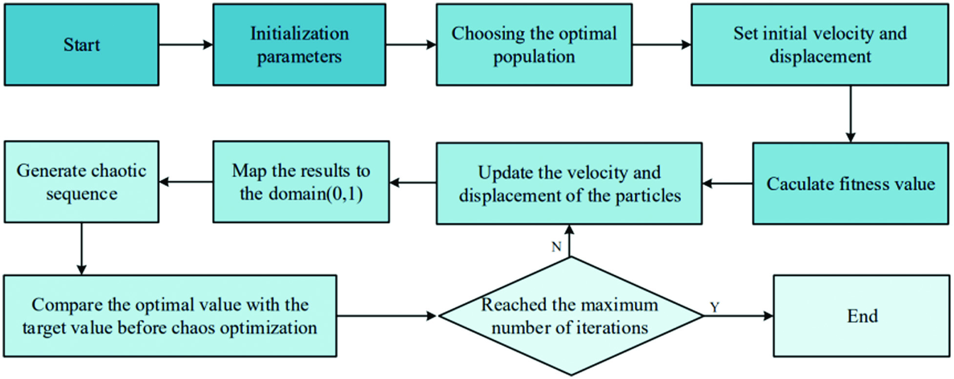

Fig. 5. Flowchart of chaotic PSO algorithm.

V.EXPERIMENT RESULTS AND DISCUSSIONS

A.SIMULATION DATA

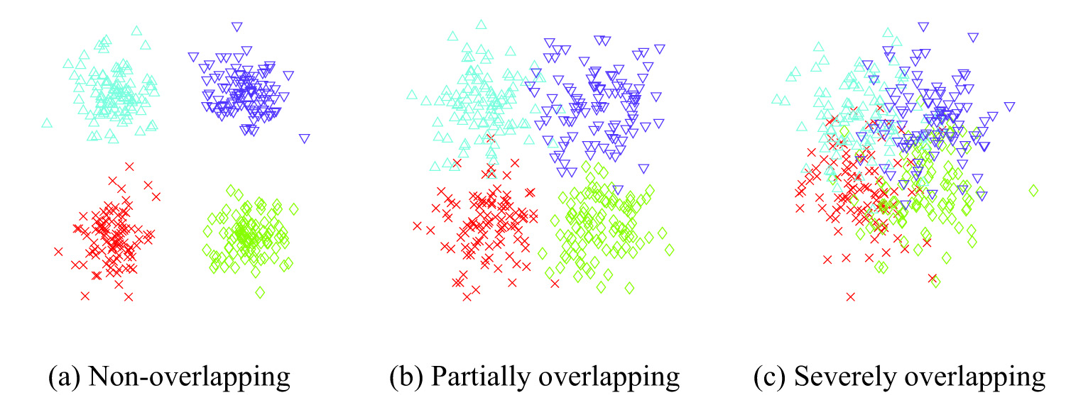
Assume $N = 400, k = 4$ . The dimension of the feature vectors is 2. Undeniably, some data may belong to more than one class simultaneously. It is difficult to assign these data to a particular class with certainty. Overlapping means that an object can belong to more than one cluster simultaneously. We conducted experiments according to different degrees of overlapping. The distribution of the data for different cases of non-overlapping, partial overlapping, and severe overlapping is shown in Fig. 6. There are four types of data in Fig. 6, represented by blue triangles, purple inverted triangles, red crosses, and green diamonds. From Fig. 6(a)–6(c), the degree of mixing of different types of data is continuously increasing. The images obtained by a good clustering method have dense samples within the same cluster and samples far enough apart between different clusters.

Fig. 6. Artificial data [24] to three different degrees.

B.ALGORITHM COMPARISON

In this study, we compared the performance of the CPSO algorithm with the FA [23] and CSA [25] algorithms. Table II shows the VRC values of these algorithms under various conditions. When there was no overlapping, the VRC values of all three algorithms were the same, at 1683.2, whether it was the best VRC value, the mean VRC value, or the worst VRC value. The best VRC values were still the same when there was partial overlapping. However, in this condition, the FA algorithm achieved the highest mean VRC value of 618.2. The mean VRC values obtained by the three algorithms were not significantly different. The CPSO algorithm had the highest worst VRC value at 583.7. For severe overlapping conditions, the FA, CSA, and CPSO algorithms achieved the highest VRC value of 275.6, with mean VRC value of 221.5, 224.0, and 222.6, respectively, and worst VRCs of 133.9, 141.8, and 144.0, respectively. Overall, the CPSO algorithm obtained the highest VRC values for different types of overlapping conditions. CPSO’s superior performance in the most severe overlapping condition compared to the other algorithms tested in the study is an important advantage. Since overlapping data are a common challenge in many practical applications, this advantage suggests that CPSO could be a valuable tool for handling real-world data that often contain varying degrees of overlap.

Table II. Experiment results for three algorithms tested

Overlapping degree	VRC $↑$	FA [23]	CSA [25]	CPSO (ours)
Non	Best	1683.2	1683.2	1683.2
	Mean	1683.2	1683.2	1683.2
	Worst	1683.2	1683.2	1683.2
Partially	Best	620.5	620.5	620.5
	Mean	618.2	616.3	617.8
	Worst	573.3	582.0	583.7
Severely	Best	275.6	275.6	275.6
	Mean	221.5	224.0	222.6
	Worst	133.9	141.8	144.0

( $↑$ means the larger, the better).

VI.CONCLUSION

An optimization algorithm based on CPSO for clustering analysis has been proposed in this paper, which has solved the limitations of traditional PSO in clustering analysis. The algorithm has introduced chaos factors into the PSO algorithm, which has prevented falling into local optimal solutions while ensuring global search. Comparing the VRC values of our proposed method with other methods, it has been found that our proposed method has better performance in different lapping conditions. In the future, we will improve the VRC values of this promising method in overlapping data. Also, many other optimization algorithms [36] will be tested.

CPSO: Chaotic Particle Swarm Optimization for Cluster Analysis