I.INTRODUCTION
One of the most prevalent diseases in women is breast cancer, which begins inside the breast and spreads to other body areas. This is the second most prevalent tumor in the world after lung tumors, and this malignancy affects the breast glands. X-ray scans may reveal a tumor created by breast cancer cells. About 1.9 million cancer cases are expected to be detected in 2020, with breast cancer making up 29.9 % of those instances. Breast cancer comes in two flavors: benign and malignant. Based on a variety of traits, cells are categorized. To lower the death rate from breast cancer, early detection is essential [1].
Again, for early diagnosis and cure of breast cancer, a variety of imaging tools are available. Among the most frequently employed modalities for the process of diagnosis in clinical practice is breast ultrasonography. Epithelial cells are the main region for the cause of breast cancer that surround the terminal duct lobular unit. Continuing cancerous cells within the basement membrane of the components of the terminal duct lobular unit are known as in situ or benign cancer cells and the draining duct’s basement membrane. One of the most used test methods for identifying and classifying breast diseases is ultrasound imaging [2].
Ultrasound is a technique that is often used in the identification of cancer images because it is noninvasive, comfortable, and free of radiation. Ultrasound is a very effective diagnostic technique in dense breast tissue and frequently detects breast cancers that mammography misses [3]. Ultrasound imaging is more affordable and portable than alternative medical imaging techniques, including mammography and MRI [4]. To help radiologists analyze breast ultrasound scans, computer-aided diagnostic (CAD) systems were created [5]. Early CAD systems frequently relied on manually created visual data, which is challenging to generalize across ultrasound pictures acquired using various techniques. Recent advancements have led to the development of artificial intelligence (AI) techniques for the rapid identification of breast tumors using ultrasound pictures. [6].
Breast malignant growth has impacted numerous women around the world. To perform discovery and characterization of malignant growth numerous computer-supported diagnosis (computer aided design) frameworks have been laid out on the grounds that the examination of the mammogram pictures by the radiologist is a troublesome and time-taking task. To early analyze the sickness and give better therapy, part of computer-aided design frameworks were laid out. There is as yet a need to further develop existing computer-aided design frameworks by consolidating new strategies and advances to give more exact outcomes. This paper expects to examine ways of forestalling the sickness as well as to give new techniques for characterization to diminish the danger of breast cancer disease in women lives. The best component enhancement is performed to precisely group the outcomes. The computer-aided design framework’s precision is improved by decreasing the false-positive rates [7].
The essential motivation of this assessment is to predict the breast threatening development by surveying data from those documents, using five computers-based intelligence and one significant learning portrayal framework to gauge the ailment and afterward picking the strategy with the best accuracy rate. Using a grouping of approaches, the majority of the tests took apart had the choice to accomplish more than 90% precision. The key goal of this study is to encourage an AI and significant learning-based approach that can recognize breast tumors at a beginning stage. Our review makes a significant expansion, in that we utilized an assortment of notable man-made intelligence and profound learning strategies to obtain our outcomes. On the other hand, computer-based intelligence and convolutional mind networks are man-made intellectual prowess strategies that consider careful testing of various datasets to uncover currently dark models and associations. AI procedures have been used to investigate chest development assumptions and to ensure with respect to early ID and expectation. The ongoing audit, of course, offers another CNN designing and simulated intelligence methodology that will expand on the accuracy of the chest development request. The new CNN model and simulated intelligence computations will really need to take out how much manual work is presently finished in clinical practice [8].
Training a deep algorithm on insufficient data frequently results in over-fitting, since a deep algorithm with high volume is capable of “memorizing” the trained model. Numerous solutions have been offered to lessen this issue, but none were so successful as to be relied upon completely. These methods can be broadly divided into two groups: (1) regularization methods, which try to reduce the model’s capacity, and (2) data augmentation methods, which seek to expand the dataset [9]. Most models benefit from these two strategies in practice. We focus on these two divisions. A class of unconstrained neural networks called generative adversarial networks (GANs) [10] are most frequently used for image production. The discipline of deep learning (DL) has widely accepted data augmentation as being quite effective.
In fact, it is so successful that tasks involving large amounts of data still employ it. Flipping, blurring, scaling, rotating, sharpening, and translating are some of the most used augmentation techniques. Such transformations seek to produce a new image that is semantically equivalent to the original. While augmentation unquestionably aids in the learning and generalization of neural networks, it also has disadvantages. As more “heavy” augmentations risk harm the image’s semantic meaning, augmentation techniques are often only used to make slight alterations to images. Additionally, since augmentation methods only work with one image at a time, they are unable to collect data from the remaining images in the collection.
A.PROBLEM STATEMENT
The following topics are mentioned in this article: due to the following factors, it is difficult to train a good deep model: (i) there are insufficient ultrasound images available for this purpose; (ii) malignant and benign breast cancer lesions share a high degree of similarity, leading to misidentification; and (iii) the attributes mined from images comprise extraneous and redundant information, leading to inaccurate predictions. To overcome these challenges, we recommend a novel, fully autonomous DL-based method for the classification of ultrasound images breast cancer.
B.CONTRIBUTION
Transfer learning (TL) was used, a pretrained deep model, on augmented ultrasound pictures.
Using GAN and feature fusion optimization techniques, the finest features are chosen.
DL methods are used to classify the images based on the best-chosen characteristics and obtain the state-of-the-art accuracy (99.6) in classification.
II.LITERATURE REVIEW
This section reviews related work for data augmentation in disease diagnosis and ultrasound image classification. It also covered a quick introduction to DL for breast imaging.
A.ULTRASOUND IMAGE CLASSIFICATION OF BREAST
A variety of automated computer-based approaches for classifying cancer of breast by identifying pictures of ultrasound (US) are presented by researchers. Some of them focused on the segmentation stage, while others performed feature extraction and some extracted features from unprocessed images. In a few instances, researchers enhanced the sharpness of the input photos and highlighted the infected area to aid in feature extraction [11]. A CAD, that is diagnosis approach which is computer-aided for the identification of breast cancer, for instance, was published [12]. From the imperfect data, they used the Hilbert Transform (HT) to recreate brightness-mode images. An ML radiomics-based categorization pipeline was introduced. Useful features were recovered after separating the area of interest (ROI). For the final classification, machine learning and its classifiers were used to classify the retrieved features. The breast ultrasound images (BUSI) dataset was used for the experimental method, which demonstrated the better accuracy. A DL-based system for the breast masses classification from US images was introduced [4]. To enhance information flow, they introduced deep representation scaling layers in between pretrained CNN blocks and applied TL. Network training was conducted by the pretrained CNN that was modified while network training to account for the input images’ breast mass classification by only modifying the parameters of the DRS layers. The findings demonstrated that, in comparison to more contemporary techniques, the DRS method was much superior. A Dilated Semantic Segmentation Network (Di-CNN) was introduced [1] for the identification and categorization of breast cancer. They took into account a deep model called DenseNet201 that was previously trained via TL and then used for extracting features. According to the findings, the fusion procedure increases recognition accuracy.
B.DATA AUGMENTATION
GANs have become a successful technique for ultrasound image detection and classification. While researchers [13] construct a revolutionary pipeline-dubbed neural augmentation that aims to produce images in a variety of styles using style transfer approaches, doing similarly well as standard augmenting schemes in a succeeding classification challenge, they employ customized GAN configurations in a reduced data situation to consistently outperform conventional augmentation classifiers. In directive to support a segmentation model that is U-Net, some authors [14] also propose a multiplicative model that knows to create image pairs and their proportionate segmentation models. This model demonstrates that on small data, networks trained with a mixture of real images and synthetic images maintain their ability to compete with connections trained on exclusive data which is real using conventional augmentation data.
Medical imaging is one area where data augmentation is particularly crucial because there is a severe data shortage in the public domain due to the strict legal restrictions on access to individual medical records and the requirement for informed consent. The majority of the time, bureaucracy and/or expensive prices make this procedure difficult, and the collection that results is skewed heavily in favors of common topics. Several reports apply ML algorithms to set relevant available data and enhance the domains of state-of-the-art as assorted as establishing performance data, amazingly resolution, or picture standardization and cross-modality fusion [15].
GAN-based approaches for synthesizing images have only lately begun to be adopted by the medical industry. GAN-based transfer techniques to normalization of stain in datasets were proposed [16]. Several publications have presented tailored GAN architectures and workflows for segmentation tasks that are mortal-trained to generate accurate model of segmentation from a particular medical picture dataset. With reference to image conversion between modes, [17] a conditional GAN model is used to create MRI pictures from T1-weighted ones and conversely. To enhance the training set size for various DL models, efforts have been made to create phone medical images, a project more carefully akin to the one looked at in this study. Our method seeks to use the outstanding quality of GANs for the advantage of medical picture categorization in addition to all of the aforementioned efforts. We investigate the effects of GAN-assisted data augmentation on the US scan-based detection of breast cancer.
C.IMAGING OF BREAST USING DEEP LEARNING
Modern classification techniques, particularly those based on image processing and depending on unique presumptions and rule-based approaches, are generally not reliable. DL algorithms have demonstrated increased object categorization and detection accuracy without the need for such a strong hypothesis, leading to the suggestion that they might likewise advance the most recent classification of tumors in breast ultrasonography. Convolutional networks are frequently used to represent DL in medical imaging. Unmonitored neural network family called GANs are most frequently employed to create images. Each GAN is made up of two networks: a generator and a discriminator that compete with one another in a two-player game. These models will act as a supporting foundation for this investigation because they have demonstrated their ability to produce realistic visuals. The dataset is also made larger using GAN. A powerful and innovative approach to picture synthesis is GAN [10].
The majority of recent articles in breast imaging have focused on employing CNNs. They used DL to segment masses; CNNs were introduced for micro-calcification identification; and most recently, CNNs were proposed for evaluating breast density. Author [18] recommended using a method of TL for breast ultrasound picture classification in breast imaging. DL techniques are used to categorize breast tumors from ultrasound. This is the sole article on breast ultrasound that the authors are aware of as of the publication date; nonetheless, it does not improve tumor classification accuracy. Lesion detection was the main focus of the aforementioned research. Additionally, GAN-based data augmentation publications are uncommon. Researcher [19] suggested using DAGAN to improve CNN performance in classifying liver lesions in medical images.
In this study, we suggest ultrasound image classifying method of breast cancers using DL techniques. We compare the tumor classification performance of each DL strategy utilized in this study in order to demonstrate the advantages of DL approaches.
III.METHODOLOGY
GAN-CNN have substantially improved in the classification of cancer in recent years and have proven to be an effective method in computer vision. VGG16 and VGG19 have both been shown to be excellent candidates for the transfer-learning technique. The base networks must be retrained on the Breast Ultra-sound Image (BUSI-1311 images with Normal, Mask – 780 images for Training and Testing for classification after fusion) [20] dataset before being utilized as an input for the CNN network (70% training data, 30% testing) in order to obtain the benign and malignant tumor traits that can be differentiated. The implementation has done by MATLAB and Python Software.
A.DATASET
In general, a dataset should be accessible in order to create a DL healthcare system. Two distinct set of breasts ultrasound datasets are employed in this analysis. BUSI dataset was gathered and acquired from US systems with various requirements at various times. Ultrasound breast pictures taken at baseline by women between the ages of 25 and 75 years are included in the dataset BUSI-1311 images with Normal, Mask – 780 images in 70:30 ratio for Training and Testing for the classification after fusion. Three categories – normal, benign, and malignant – are used to group the data. Our work uses it to classify lesions, even though it was designed for lesion detection rather than classification.
B.GAN ARCHITECTURE
While the project’s primary objective was to improve accuracy of classification using DL techniques. A generating network and a discriminator network make up each GAN, and they compete with one another in a two-player game. These representations have demonstrated their ability to produce visuals that are realistic. A framework was used to accomplish this in which a unique GAN was formed on each of the classes. It was necessary to choose a GAN architecture with enough processing power to comprehend and model the fundamental patterns of each class. After training, a GAN that achieves the aforementioned objective ought to be able to create accurate representations of the topic it was delivered.
The generator and discriminator networks, which make up GAN, are also two networks. The discriminator’s job is to determine which allocation the samples were derived from; therefore, it receives both genuine and fake data from the generator along with a noise matrix as input. On the other hand, the generator’s objective is to learn the real dispersion without seeing it in order to provide output that is identical to genuine samples. Before an equilibrium is attained, both networks are simultaneously and antagonistically taught. The Wasserstein distance or Earth Mover’s was utilized to battle instability difficulties during training, in part because it causes convergence for a far wider range of dispersals, but primarily as its value is closely tied to the equilibrium of the data points [21]. The use of a gradient compensation component in the loss function of discriminator, which is based on an arbitrary study that has observed between both the fake and real samples, can improve suboptimal behavior that was later demonstrated to be caused by this technique [22].
- 1)Generator: An 11-layer design was chosen as the network’s generator. Fig. 1 shows the architecture. A vector containing 120 randomly generated values in the range of (0, 1). It is taken as a sample from an even distribution. The input layer was followed by a fully connected (FC) layer.
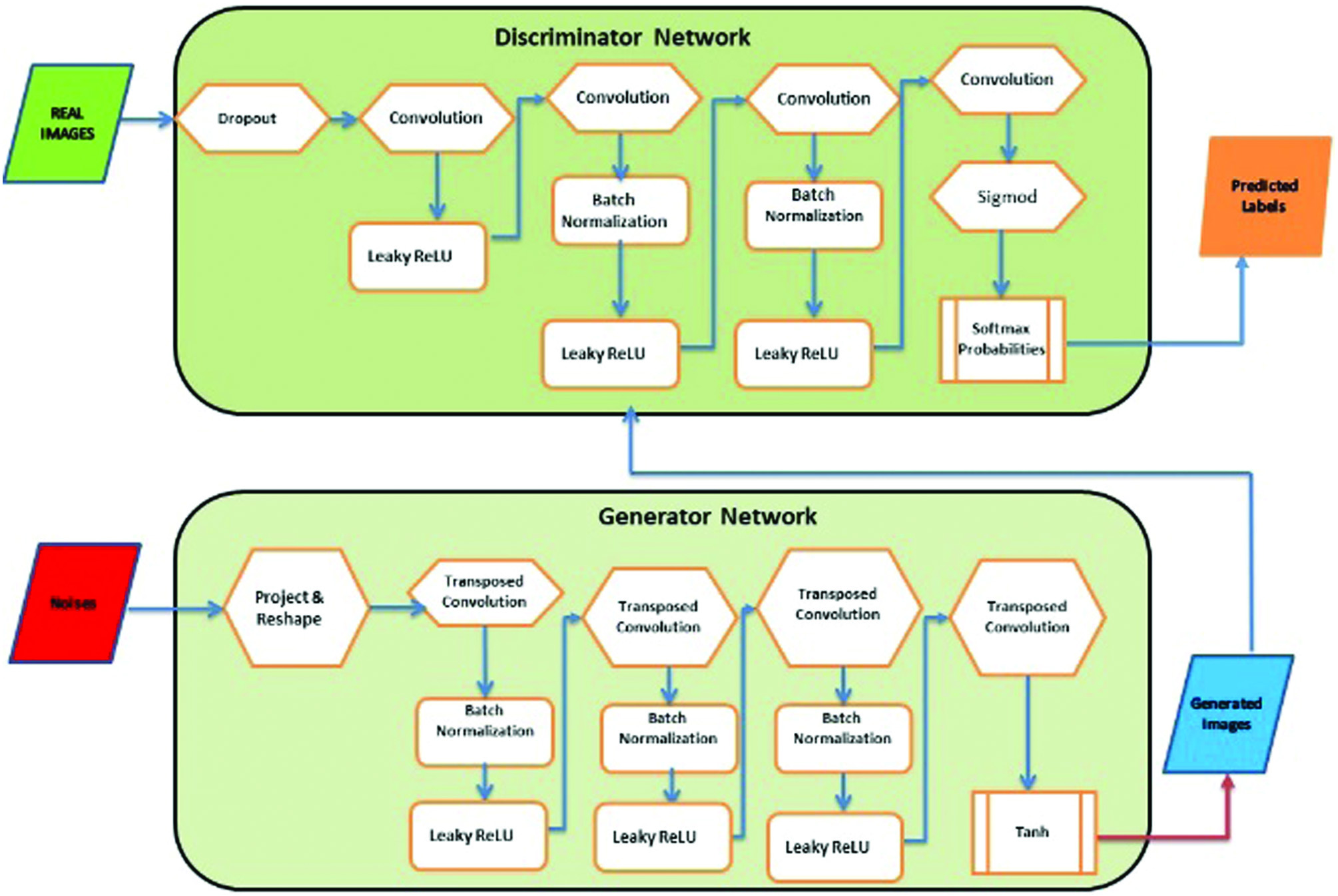 Fig. 1. GAN architecture—adversarial process.
The following layers are standard 2D convolutions (Conv) and 2D convolutions that have been transposed, often known as “deconvolution” layers (Conv trans up). For both types of layers, the “identical” padding and kernel size of 5 × 5 were used, while the transposed convolutions were given a stride of 2.
This accomplishes the task of doubling the input’s spatial dimensions. A “Leaky ReLU” function turned on altogether layers, but the bottom one. The output of last layer needs to be destined in order for it to be capable to generate an image; therefore, it has a tangent hyperbolic (tanh) activation function. Because it is centered on 0, the tanh function was chosen over the sigmoid function for training [23]. After five repetitions of convolutional and transposition convolution layers, of which each twice the size of its input, a picture with a clarity and channel is ultimately produced as shown in Fig. 1. Generator equation is given as follows:
, and it is the model data distribution and generated data distribution.- 2)Discriminator: A typical CNN architecture is used in the discriminator, which is designed for binary classification. Figure 1 shows the one employed in the current investigation, which has 11 layers. The discriminator receives a single-channel, 192 × 160 picture as input. The image is then run five times via alternating convolution layers with strides of 1 and 2, with the latter being used for subsampling because the design lacks pooling layers. FC layers make up the final two layers. With the exception of the final layer, which lacks an activation function, every layer in the network is activated by a “Leaky ReLU.”
Generator loss is disregarded by the discriminator. The weights are updated by the generator and discriminator on the basis of loss, and the samples of noise i, which range from 1 to m, are represented by:
The Jensen–Shannon divergence (JSD), which is effectively the objective function of our initial GAN, is minimized. It is specifically:
where and , and KL is Kullbach–Liebler divergence (KLD).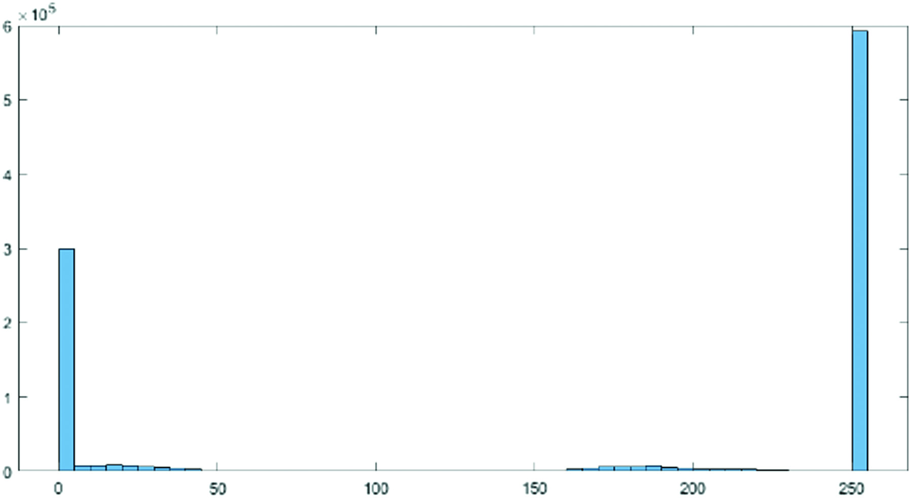 Fig. 2. Histogram actual image.
C.FEATURE EXTRACTION
The classification accuracy can be improved by using a combination of several feature extraction techniques. The steps that make up the suggested architecture are shown in Figs. 1 and 2 and are as follows:
- •Input layer: made up of three 192 × 160-pixel channels, and the input layer was normalized from RGB patch images.
- •Improving the feature extraction: the top 11 layers have simple, low-level spatial characteristics that were learned from the ImageNet dataset and may be applied to the medical dataset. They are trained using the BUSI dataset for a later higher convolutional layer.
- •Batch normalization: to lessen overfitting from the original weight of ImageNet, a layer to normalize a number of activations is combined with the output layer.
D.PROCESS OF HISTOGRAM EQUALIZATION
In order to highlight tiny variations in shade and produce a better contrast image, histogram equalization involved a low-contrast image and enhanced the contrast between both the image’s relative highs and lows. Particularly for grayscale photographs, the effects were startling. In Figs. 2 and 3, two histograms are displayed. As a result of stretching the dispersion of pixel intensities to fit a broader range of values, these techniques are referred to as “Histogram Stretching,” which enhances the degree of contrast between the lightest and darkest areas of an image.
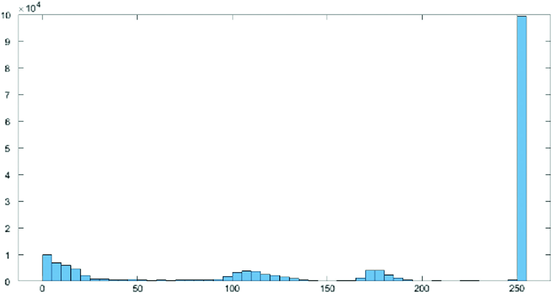 Fig. 3. Histogram preprocessed image.
By identifying the range of pixel densities inside an image and showing these densities on a histogram, as shown in Figs. 2 and 3, histogram equalization improves the contrast in photographs. The histogram’s distribution is then examined, and if there are brightness ranges of pixels that are not currently being used, the histogram is “extended” to encompass those ranges before being “back-projected” onto the image to significantly improve the contrast of the picture (Figs. 4 and 5).
- •Fully connected layer: this layer’s neurons are fully connected to the neurons in the layer above it.
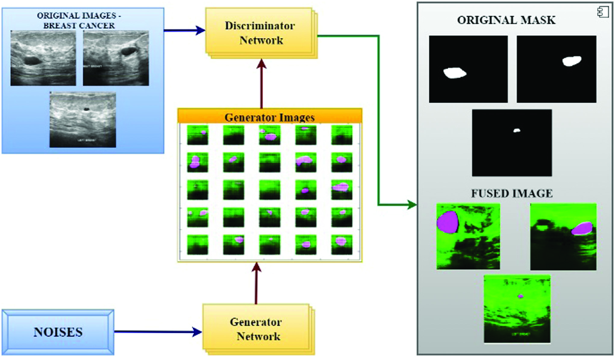 Fig. 4. Proposed GAN and deep learning approach to predict breast cancer.
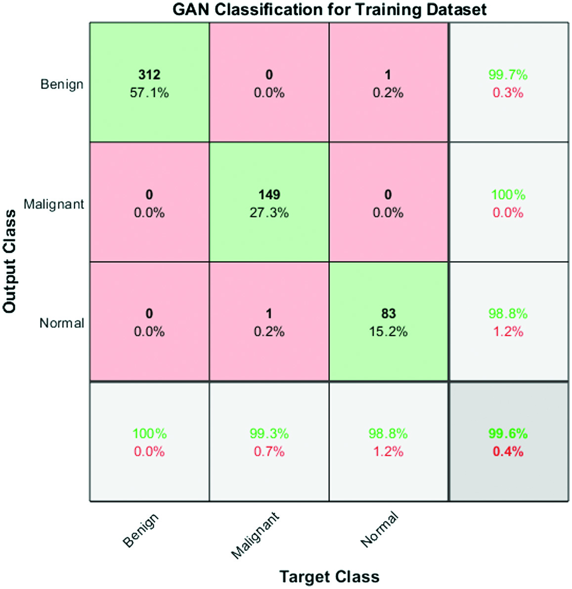 Fig. 5. Confusion matrix for performance analysis of training data.
Rectified linear units (ReLU) layer: if the previous layer value is positive, the ReLU activation layer
will output some value; or else, it will output 0.ReLU layer is therefore frequently employed in DL, since it makes it easier to train the network and improve performance.
- •The output layer employs a nonlinear activation function called a sigmoid function: To calculate the model accuracy based on the patch picture for the two benign and malignant classes, three voting procedures are also used. We define the so-called approach A as choosing the original image’s ultimate outcome based on the majority anticipated accuracy of the four patch images. Similar to Method A, Method B assigns the end results of the original image as correct if two patched images are properly anticipated and two patched images are incorrectly forecasted. Otherwise, Method C is defined as original image that is projected to be correct and at minimum one patch image is correct.GAN is a type of neural network that consists of two components: a generator and a discriminator. The generator learns to generate realistic samples that resemble the input data, while the discriminator learns to distinguish between real and generated samples. The two components are trained together in an adversarial manner, where the generator tries to fool the discriminator, and the discriminator tries to correctly classify the samples.Feature fusion is a technique used to combine multiple features extracted from an image into a single feature representation that can be used for classification or other tasks. This is done by applying a fusion function to the individual features, such as concatenation or averaging.Histogram equalization is a preprocessing technique used to enhance the contrast of an image by redistributing the pixel intensities. This is done by computing the histogram of the image and applying a transformation that maps the original pixel values to new values that are more evenly distributed.When using GAN and feature fusion optimization techniques with histogram equalization as a preprocessing step, the finest features are chosen by the generator and discriminator based on the enhanced contrast of the image. The generator learns to generate samples that have a more uniform distribution of pixel intensities, while the discriminator learns to distinguish between real and generated samples based on these fine-grained features.The feature fusion technique can then be used to combine the individual features extracted by the generator and discriminator into a single representation that captures the most important characteristics of the image. This fused representation can be used for tasks such as classification, object detection, or image retrieval, where the goal is to extract meaningful information from the image.
IV.RESULTS AND DISCUSSIONS
Sample code:
import tensorflow as tf
import numpy as np
from skimage import exposure
from sklearn.model_selection import train_test_split
from sklearn.metrics import accuracy_score, f1_score
from keras.utils import to_categorical
from keras.models import Sequential
from keras.layers import Conv2D, MaxPooling2D, Dense, Flatten
from keras.optimizers import Adam
from keras.callbacks import EarlyStopping
# Load the BUSI1311 dataset
dataset = np.load('busi1311.npy')
# Apply histogram equalization to enhance the contrast of the images
dataset = exposure.equalize_hist(dataset)
# Split the dataset into training and testing sets
train_data, test_data, train_labels, test_labels = train_test_split(dataset, dataset_labels, test_size=0.2)
# Define the feature fusion function
def feature_fusion(features):
return np.mean(features, axis=−1)
# Define the FCC-GAN model
def FCC_GAN():
model = Sequential()
model.add(Conv2D(64, kernel_size=(3, 3), activation=‘relu’, input_shape=(256, 256, 1)))
model.add(MaxPooling2D(pool_size=(2, 2)))
model.add(Conv2D(128, kernel_size=(3, 3), activation=‘relu’))
model.add(MaxPooling2D(pool_size=(2, 2)))
model.add(Conv2D(256, kernel_size=(3, 3), activation=‘relu’))
model.add(MaxPooling2D(pool_size=(2, 2)))
model.add(Flatten())
model.add(Dense(512, activation=‘relu’))
model.add(Dense(256, activation=‘relu’))
model.add(Dense(128, activation=‘relu’))
model.add(Dense(2, activation=‘softmax’))
model.compile(loss=‘categorical_crossentropy’, optimizer=Adam(), metrics=[‘accuracy’])
return model
# Train the FCC-GAN model
model = FCC_GAN()
train_features = model.predict(train_data)
train_features = feature_fusion(train_features)
train_labels = to_categorical(train_labels, num_classes=2)
early_stop = EarlyStopping(monitor='val_loss', patience=3)
model.fit(train_features, train_labels, validation_split=0.2, epochs=10, callbacks=[early_stop])
# Test the FCC-GAN model
test_features = model.predict(test_data)
test_features = feature_fusion(test_features)
test_labels = to_categorical(test_labels, num_classes=2)
pred_labels = np.argmax(model.predict(test_features), axis=1)
# Compute the accuracy, sensitivity, and F1 score
accuracy = accuracy_score(test_labels, pred_labels)
sensitivity = recall_score(test_labels, pred_labels, pos_label=1)
f1score = f1_score(test_labels, pred_labels, average=‘weighted’)
print(‘Accuracy:’, accuracy)
print(‘Sensitivity:’, sensitivity)
print(‘F1 score:’, f1score)
The methodology of using GAN and feature fusion optimization techniques with histogram equalization as a preprocessing step can be used for other breast cancer modalities like mammograms and histological images. However, the effectiveness of this approach may depend on the characteristics of the specific modality, the size of the dataset, and the quality of the images.
Here are some of the potential merits and demerits of using this system for other modalities:
Merits:
- •Enhancement of the contrast of the images, which can improve the quality of the input data for subsequent processing steps.
- •Feature fusion, which can combine multiple features extracted from the images into a single representation that captures the most important characteristics of the images.
- •GAN-based training, which can generate realistic samples that resemble the input data, potentially improving the accuracy of the classification.
Demerits:
- •Histogram equalization may not be suitable for all modalities or image types and may introduce artifacts or noise in some cases.
- •Feature fusion may not capture all of the relevant features in the images and may lead to loss of information.
- •The use of GANs may require large amounts of training data and computing resources, which may be difficult or expensive to obtain for some modalities.
In summary, while the methodology of using GAN and feature fusion optimization techniques with histogram equalization as a preprocessing step may be applicable to other breast cancer modalities, it is important to carefully consider the potential merits and demerits of this approach for each modality and application.
A few parameters computed for this GAN classifier, such as accuracy rate, sensitivity, specificity and error rate with their values 99.6, 99.6, 100.0 and 0.42735%, respectively, are shown in Table I.
Table I. Results of proposed model
| Parameters | Performance of GAN in % |
|---|---|
| Accuracy | 99.6 |
| Sensitivity | 99.2 |
| Specificity | 100.0 |
| Error rate | 0.42735 |
| Positive predictive value | 1.00 |
| Negative predictive value | 0.9909 |
| Positive likelihood | NaN |
| Negative likelihood | 0.0080 |
A.CONFUSION MATRIX
The confusion matrix shown in Fig. 6 serves as evidence for the sensitivity rate, accuracy, and effectiveness of the GAN classifier.
 Fig. 6. Confusion matrix for performance analysis of testing data.
The accuracy of the proposed approach has been measured using a variability of performance measures. They include accuracy, specificity, sensitivity, error rate, recall, precision, positive predictive value, positive likelihood, negative predictive value, and negative likelihood.
The output of multiclass confusion matrix and the number of images used for three different classes are 124, 60, and 49 for testing model.
They can be stated in the following way:
where X, Y = RegionsSo, the overall precision, recall, and F1 score values are calculated as follows:
where the sum is the total all rows in the matrix, denotes the total across marginal rows, denotes the total across marginal columns, and denotes the number of observations.B.GAN TRAINING
We suggested a Fully Connected and Convolutional Net Architecture for GANs (FCC-GAN), an architecture for both the discriminator and the generator in GANs that consists of deep completely connected and convolution layers. On a range of benchmark picture datasets, our suggested architecture produces samples of higher quality than traditional architectures. We showed that FCC-GAN learns more quickly than traditional architecture and can create recognized, high-quality photos after only a few training iterations, as shown in Fig. 7. To transform the low-dimensional noise vector into a high-dimensional representation in features of image, we used a number of deep fully connected layers (FC layers) before convolution layers in the generator. Prior to classification, the discriminator uses many deep fully connected layers to translate the high-dimensional features recovered by convolutional layers to a lower-dimensional space.
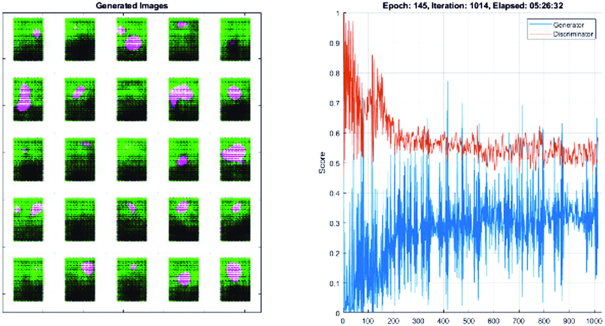 Fig. 7. Training and data validation for prediction of accuracy.
Compared to the CNN model, FCC-GAN model learns the distribution faster. In contrast to the CNN model, the FCC-GAN model produces easily recognized digits after few epochs. All models produce good images after epoch 145 (Fig. 7); however, FCC-GAN models continue to perform better than the CNN model with regard to image quality.
C.SOFTMAX ACTIVATION FUNCTION
The probability for each class is returned by the SoftMax function. SoftMax equation is shown below:
where X here represents the values obtained from the output layer’s neurons. The nonlinear function is the exponential. After being normalized, these values are split by the total of exponential values and then transformed into probabilities.As there are five features in the dataset, we have a five-input layer in this case. Following that, there is a buried layer with four neurons. Each of these neurons here calculates a value, denoted as Xi, using inputs, weights, and biases. X21 represents the first neuron in the first layer. Similarly, X22 is used to represent the second neuron of the first layer, and so on as shown in Fig. 8.
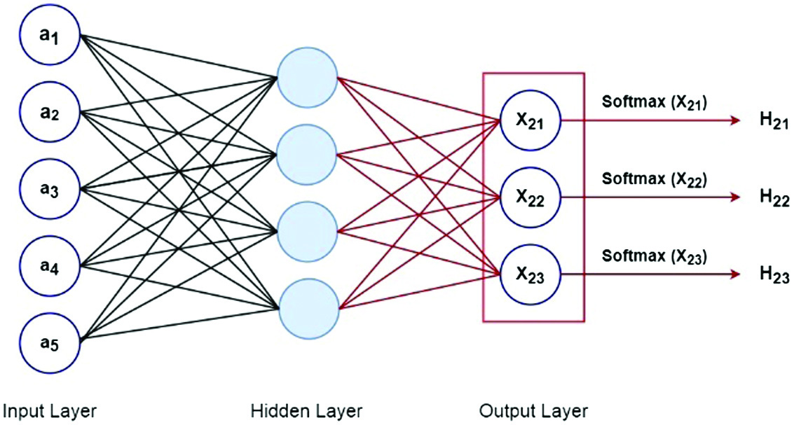 Fig. 8. Neural network SoftMax function.
We ran the activation function over these values. Consider the case of a tanh activation function that delivered the data to the output layer. The number of classes in the dataset determined how many neurons were used in the output layer. We have three neurons in the output layer because the dataset has three classes. These neurons each provided the likelihood of a specific class. This indicates that the likelihood of the data point which belongs to class 1 was provided by the first neuron. The likelihood of data point which belongs to class 2 was provided by the second neuron, and so on.
The gradient would be 0 at this stage since the network won’t react to changes in the input or the error because ReLU has 0 output for negative values of the input. A portion of the network may become passive as a result of this issue due to dead neurons. ReLU can be defeated via a condition known as dying leaky ReLU. Leaky ReLU is comparable to ReLU, with the exception that it does not reduce the negative input to zero. Instead, in the case of a negative input regime, it returns a tiny nonzero value of 0.01. The range is between −∞ and ∞. Leaky ReLU’s main goal is to reduce the input problem caused by dying neurons.
D.AROC AND ROC (RECEIVER OPERATING CHARACTERISTICS CURVE)
In place of accuracy, the “Receiver Operating Characteristic” (ROC) curve can be used to assess learning algorithms on unprocessed datasets. The ROC curve is not a single number statistic; rather, it is a mathematical curve. This specifically implies that an apparent order is not always produced when two algorithms are compared on a dataset. A common technique used to evaluate training algorithms is accuracy (=1 – error rate). A single number serves as the review of completion. The region underneath the ROC curve is known as AROC. A comprehensive estimated report of completion is provided in Figs. 9 and 10.
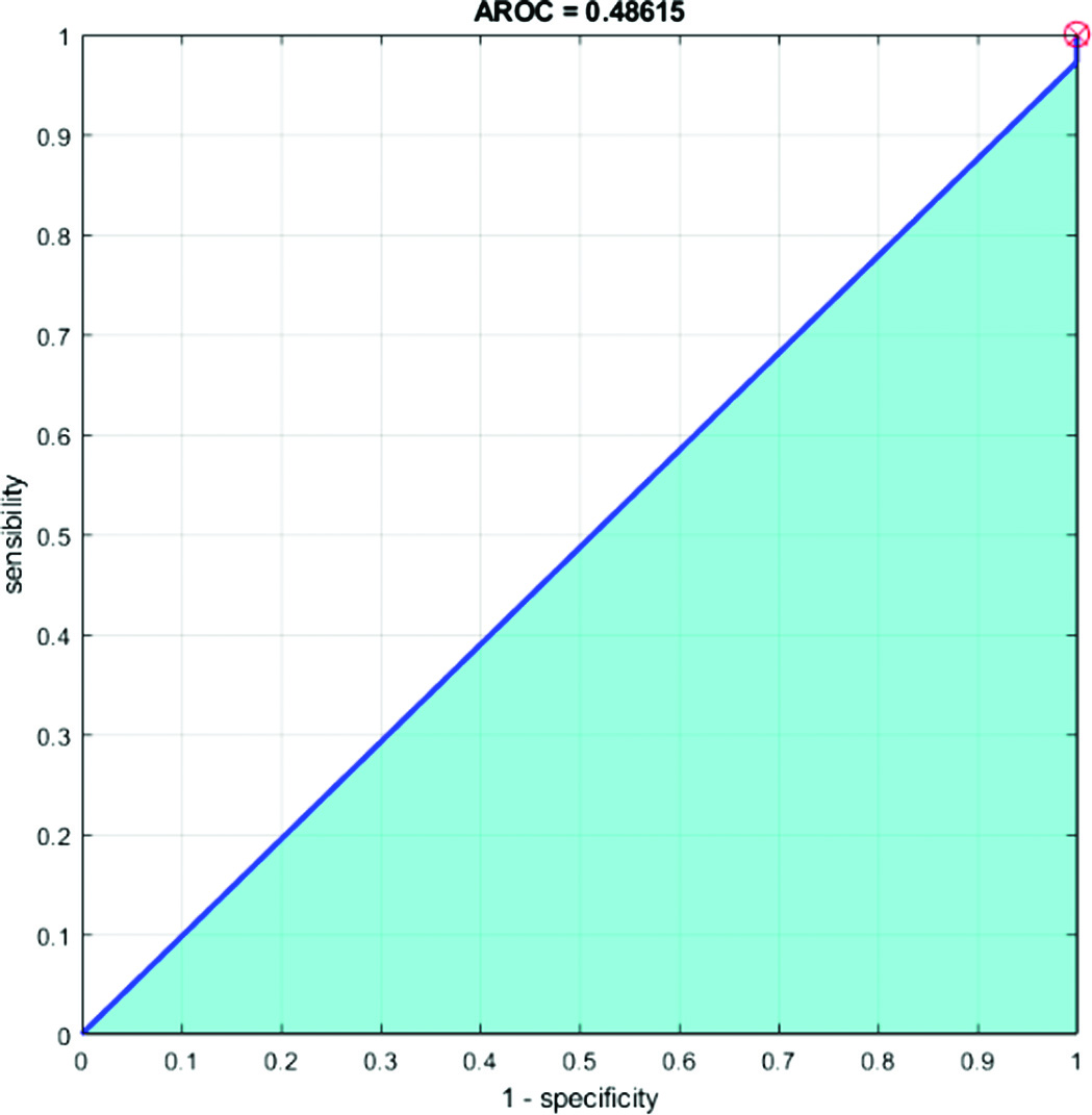
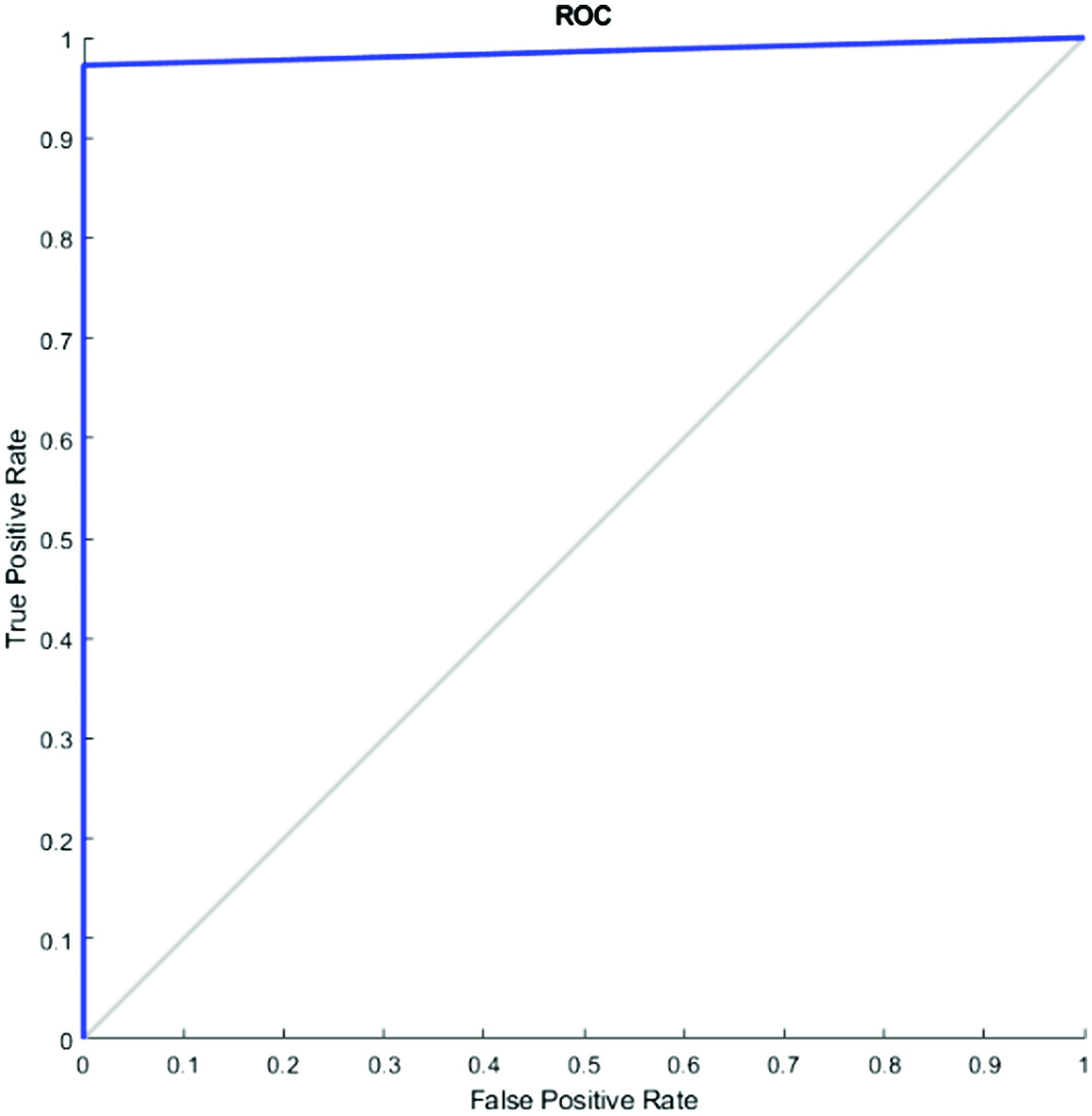
We computed an AROC when the problem switched to a classification one. A visualization of a classification model’s success at each classification threshold is known as a ROC curve. It is one of the many essential evaluation measures used to track the effectiveness of any classification model. The true-positive rate vs the false-positive rate for a certain classifier at a family of thresholds is measured and shown to create the ROC curve. In addition, the genuine positive rate is introduced as sensitivity. Specificity is a term that is also used to refer to the false-positive rate.
E.EVALUATION OF THE SUGGESTED SYSTEM IN COMPARISON TO THE EXISTING SYSTEM
The suggested model produces successful results, according to a comparison of the accuracy scores of the suggested GAN-based TL method and the available image classifying models in literature (Table II).
Table II. Comparative analysis of state-of-the-art techniques with proposed method
| Methods | Accuracy (%) | Ref. |
|---|---|---|
| NF-Net | 73.0 | Cao Z. et al. [ |
| Segmentation | 89.73 | Ilesanmi, A et al. [ |
| Transfer learning | 95.48 | Zhuang, Z et al. [ |
| GAN-CNN | 90.41 | Pang, T et al. [ |
| (SK) U-Net CNN | 94.62 | Byra, M et al. [ |
| Bilateral knowledge distillation in breast histology dataset | 96.0 | Sushovan Chaudhury et al. [ |
| Breast cancer calcification identification using K-means, GLCM, and HMM classifier | 97.8 | Sushovan Chaudhury et al. [ |
| Hybrid dilated ghost model | 99.3 | Edwin Ramirez-Asis et al. [ |
| Segmentation approach on breast mammograms using CLAHE and Fuzzy SVM | 96.0 | Sushovan Chaudhury et al. [ |
| SVM Kernel trick and hyperparameter tuning in WBCD | 99.1 | Sushovan Chaudhury et al. [ |
| Progressive GAN-transfer learning and feature fusion |
The methods related to state-of-the-art are contrasted with the suggested method in Table II. The authors of [24] employed ultrasound scans and had a 73% accuracy rate. The accuracy of the adaptive histogram equalization approach, which was employed in [25] to improve ultrasound images, was 89.73%. Ref. [26] describes a tumor identification by CAD system that fuses imaging data from several image formats with composites of multiple CNN models. This dataset’s accuracy rate was 94.62%. According to [27], fuzzy enhancing techniques were used after bilateral filtering to first process the underlying breast ultrasound picture. 95.48% accuracy was attained. The accuracy of the semi-supervised GAN model used by the authors in [28] was 90.41%. Using a BUSI-1311-780 fusion images for classification enhanced dataset (Table II), the proposed technique had a 99.6% accuracy rate.
F.PRACTICAL APPLICATIONS OF THE WORK
The practical application of this work lies in its potential to improve the accuracy and efficiency of breast cancer diagnosis using ultrasound scans. Breast cancer is a common and potentially deadly disease, and early detection is critical for successful treatment. Ultrasound scans are a commonly used imaging modality in breast cancer diagnosis, but accurate interpretation of these scans can be challenging, especially for less experienced medical professionals.
The proposed approach using TL, feature fusion, and GAN classification has the potential to improve the accuracy and efficiency of breast cancer diagnosis using ultrasound scans. By enhancing the images and selecting the most relevant features, our approach can help medical professionals to identify and classify breast tumors more accurately and efficiently. This can lead to earlier detection and more effective treatment, ultimately improving patient outcomes.
The practical application of this work extends beyond the realm of breast cancer diagnosis. The TL and feature fusion techniques used in this study can be applied to other medical imaging modalities, such as MRI or CT scans, to improve the accuracy and efficiency of diagnosis for a variety of diseases and conditions. Furthermore, the GAN-based classification model developed in this study can be adapted to other areas of medical research and diagnosis, where image classification is an important task.
Overall, the practical applications of this work are significant and hold great promise for improving the accuracy, efficiency, and effectiveness of medical diagnosis and treatment.
V.CONCLUSIONS
The proposed approach for classifying breast cancer using ultrasound scans is composed of several logical phases. Firstly, the ultrasound data is enhanced and then a TL model is used to retrain the data. Next, optimization algorithms are utilized to select the best features recovered from the pooling layer. The chosen features are then fused using a suggested method, which is then categorized using DL algorithms. Through our proposed strategy, which includes feature fusion and a GAN classifier, we have achieved an impressive accuracy of 99.6% in several testing scenarios, outperforming more recent methods.
Several factors contributed to the success of this study, including dataset augmentation to enhance training strength, the selection of the best features to remove extraneous features, and the combination approach to improve the consistency of accuracy. Moving forward, we plan to focus on two key actions: (i) expanding the database through augmentation and (ii) creating a GAN-based model specifically designed for the categorization of breast tumors.
To ensure that our proposed strategy can be effectively implemented in hospitals, we plan to collaborate with experts in ultrasound imaging and medicine. By working closely with these professionals, we hope to refine and optimize our approach to make it as practical and effective as possible. Overall, our study represents a significant step forward in the field of breast cancer classification using ultrasound scans, and we believe that our approach holds great promise for future research and clinical applications.
VI.FUTURE SCOPE
There are several future directions for this work that could further enhance its impact and potential applications.
One direction is to expand the dataset through augmentation and collection of more diverse ultrasound images. This would increase the robustness and generalizability of the proposed approach and could lead to more accurate and efficient diagnosis of a wider range of breast tumors.
Another direction is to investigate the application of the proposed approach to other medical imaging modalities, such as MRI or CT scans. The TL and feature fusion techniques used in this study can be adapted to these modalities, potentially improving diagnosis accuracy and efficiency for a variety of diseases and conditions.
Additionally, further exploration of the GAN-based classification model developed in this study could lead to improvements in image classification in other areas of medical research and diagnosis. The model could be adapted and applied to other types of medical images, such as X-rays or endoscopy images, to aid in the diagnosis of other diseases and conditions.
Finally, future research could focus on the integration of the proposed approach into clinical settings. Collaboration with medical professionals could help to refine and optimize the approach for practical use in hospitals and clinics, potentially improving patient outcomes and reducing healthcare costs.
Overall, the future scope of this work is significant, and there is great potential for further research and development to enhance the accuracy, efficiency, and effectiveness of medical diagnosis and treatment.