I.INTRODUCTION
Colon and rectal cancer (CRC), which accounts for the third-highest diagnostic rate, is the second-deadliest cancer in the United States. Rectal cancer has different environmental correlations as well as separate genetic risk factors from colon cancer. The normal rectal epithelium must undergo a series of somatic (acquired) or germline (inherited) genetic alterations over a period of 10–15 years in order to develop into a dysplastic lesion and then invasive cancer. Pathological staging and the results of preoperative care are the two most important prognostic indicators for rectal cancer. Rectal cancer is brought on by the development of malignant cells in the rectum, a section of your large intestine. Rectal cancer can affect both men and women, although it affects men far more frequently.
The initial stage of rectal cancer is when it has just recently begun to penetrate the layers of the rectal wall and has not yet spread to nearby areas. Patients with rectal cancer in Stage I were not permitted to show any symptoms or warning signs. This makes it essential to routinely screen for colon cancer. Despite not having progressed beyond the rectum, Stage I rectal cancer has advanced into the deeper layers of the rectal wall. Cancers that were a component of polyps are included in this stage. There might not be a need for further treatment if the polyp is entirely removed during the colonoscopy, and there is no malignancy in the polyp’s margins. You could be told to have further surgery if the polyp’s malignancy was a high grade or if there were cancer cells at its margins. Unless the surgeon discovers the cancer is further advanced than initially believed before surgery, additional therapy is often not required after these surgeries. If cancer is further advanced, chemo and radiation treatment are frequently administered. The most often used chemotherapy medicines are capecitabine and 5-FU. Chemotherapy along with radiation treatment may be used to treat you if your health prevents you from having surgery.
Despite decreasing mortality over the past decades, rectal cancer is still the third-most diagnosed deadly disease in the United States as per CDC data available. The latest data reports witness the diagnosis of new 142, 462 cases of bowel cancer in the United States. As per reports, 36 new cases of rectal cancer and 13 new deaths are reported for every 100,000 people. Therefore, it is stated that one of every four deaths is only because of rectal cancer, thereby the top leading cause of death in the United States [1] (Fig. 1).
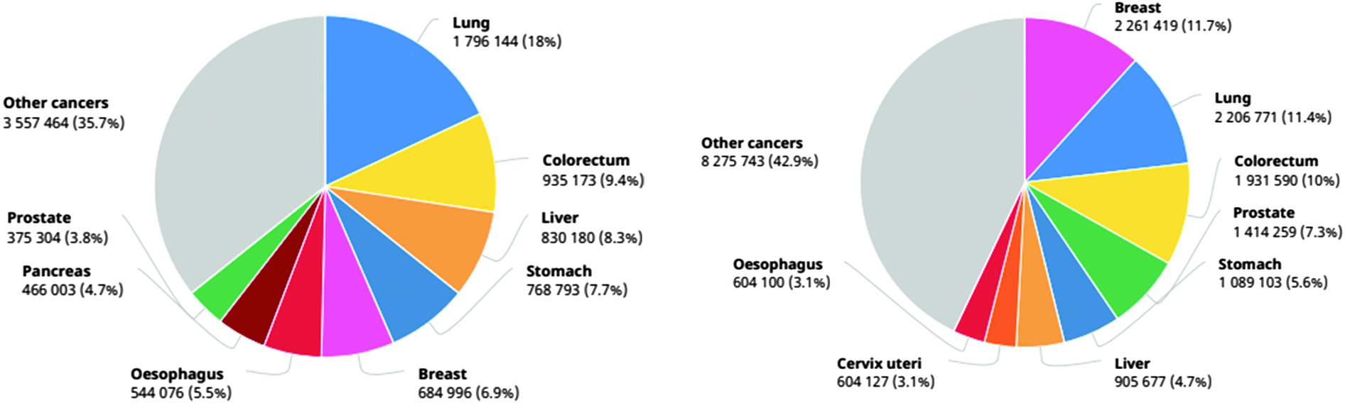 Fig. 1. Number of diagnosed and death cases in 2020 (source: GLOBOCON 2020).
Today, the International Agency for Research on Cancer (IARC) publishes the most recent figures on the cancer burden worldwide. The IARC Global Cancer Observatory’s GLOBOCAN 2020 database, which is available online, gives projections for 2020 of incidence and death rates for 36 different forms of cancer across all cancer sites combined in 185 different countries. The key findings of the GLOBOCAN 2020 report that are important to the surgical oncology community include the rising global burden of cancer, global disparities in cancer incidence and mortality in different parts of the world, and the impact of the Human Development Index (HDI) on cancer incidence and the anticipated global cancer burden by 2040.
For providing proper treatment to the patient, it is mandatory that cancer would be diagnosed at an early stage, which ultimately increases the chances of successful cancer treatment. Discussing about the early diagnosis, the two main stages are downstaging and screening. Diagnosis and downstaging is the process of detecting the early cancer stage in symptomatic individuals, whereas screening means testing healthy persons regardless of any symptoms’ visibility. Rapid care of patients is crucial in the early diagnosis of cancer, and it applies to all types of cancer. However, screening is only relevant to a few types of cancers only such as colorectal, breast cancer, and cervical cancer [2]. Adenocarcinoma is the most common kind of rectal cancer, affecting the majority of patients. There are many additional, less common tumor kinds. Treatment for these additional rectal cancer subtypes may differ from that for adenocarcinoma. Most occurrences of rectal cancer are caused by adenocarcinoma. This malignancy affects the cells that line the inner surface of the rectum. Hormone-producing cells in the intestines are the origin of carcinoid tumors. A malignancy of the immune system is lymphoma. Although it can begin in the rectum, the lymph nodes are where it usually begins. About 5% to 10% of people get colon cancer due to specific inherited mutations in their DNA, which are transferred from parents to children. If you want to discover if you have inherited DNA mutations that might raise your chance of developing cancer, MSK’s specialists might offer genetic testing. The decision to get this testing depends on how much danger you are in. Discussing the major obstacles faced in cancer detection and its early diagnosis treatments, diagnosis techniques, and methods lack in proving accurate results at the time of detection, which leads to detection at a later stage and ultimately reduces the chances of patient’s recovery at that stage. Some other major causes are as follows [3,4]:
- •low quality of diagnosis or detection;
- •low quality of treatment and services for patients;
- °errors in diagnosed results
- °ambiguous referral pathways
- °Long waiting list due to the slow working of diagnostic techniques.
Endoscopic, tumor marker, endoscopic ultrasonography, histopathological, and imaging diagnosis are the present date methods for early diagnosis of cancer [5]. But, these approaches have some limitations which create obstacles in getting accurate results of cancer diagnosis like time issues, and specialized and proficient trainers required in the medical field to handle technical equipment and analytical necessities [6]. The markers methods for examining tumor is recently available; however, this method is not accurate enough to detect all cases in the early stage, which eventually creates obstacles in providing timely therapy to the patients. Therefore, there is a need for creating fast and accurate methods for early cancer detection or evaluation.
Cancer is now widely acknowledged to be a disease of change—a condition characterized by plasticity and heterogeneity—that arises at the genetic, phenotypic, and pathological levels and proceeds through several clinical stages. We are aware of the significance of the systemic and local tumor environments in how the illness appears and evolves, in addition to deciphering the genetic fingerprint and molecular makeup of a particular cancer type. Recent years have seen a particularly strong increase in the interaction between the immune system and the immunological tumor microenvironment. Indeed, we now understand that the local and systemic environment, as well as the growth of cancer and its heterogeneity, play critical roles in the development of the illness as well as in how well or poorly a patient responds to treatment and how likely they are to experience recurrence.
Technological developments like integrated “-omics,” single-cell methods, imaging, and next-generation sequencing have made it feasible to profile many tumor forms at a scale and resolution that were previously impossible. Big data generation and sharing capabilities are profoundly changing how this disease is recognized and handled. The development of targeted therapies and the idea of precision oncology—treatment customized to the individual patient, aiming to hit cancer-specific vulnerabilities—have resulted from a more detailed understanding of the molecular drivers of cancer and the intrinsic or extrinsic vulnerabilities of tumor cells, as well as from the addition of next-generation sequencing testing to clinical practice. This should help to reduce toxicities and improve the quality of life for patients receiving treatment.
A medical professional’s time is freed up so that he may concentrate on tasks that cannot be automated thanks to artificial intelligence (AI) in the healthcare sector. The most common use of AI and digital industrialization is data management. Robots can collect, store, reformat, and analyze data to give quicker and more reliable access, while AI can manage medical records and other types of data. Another intriguing use of AI and the IoMT is in consumer-focused mobile health apps. In the creation of healthcare apps, AI/ML technology may help physicians with diagnosis and foresee when patients are becoming worse, allowing for the initiation of medical intervention before the patient needs to be hospitalized and reducing costs for both hospitals and patients.
AI adoption in the medical field has led to an unprecedented change. AI assists the pathologist in the accurate reviewing of results by using various state-of-the-art techniques [7]. As per experts, accurate detection of early symptoms is really important for successful therapy; therefore, detection at an early stage is mandatory in the entire procedure. On the other hand, a delay in detection leads to complications along with an increase in treatment costs [8,9]. The three machine learning approaches—supervised, semi-supervised, and unsupervised—that are best suited to the data at hand are also employed to diagnose cancer. Talking about unsupervised learning, the unlabeled corpus is trained to examine the patterns for detecting cancer disease. But sometimes these data are excluded whenever working on labeled data. Early cancer detection is crucial since it lowers the likelihood that a cancer patient will pass away. Microarray DNA technology is used to create data from tissues; these data comprise genes/attributes in extremely high numbers and samples in very small numbers, which makes it difficult to predict the classifier. To handle the difficulty of processing a huge number of genes/attributes, various machine learning methods that focus more on feature selection were developed. Data without labels are necessary for the unsupervised learning approach. Based on the training data, an implicit model is developed to classify unidentified samples. No tagged training data is necessary for unsupervised deep learning models. These models analyze the inherent characteristics of the data based on specific pertinent characteristics to group comparable data. These models are typically employed for feature reduction and clustering reasons. The two unsupervised deep learning models employed most frequently are the autoencoder (AE) and restricted Boltzmann machines (RBMs).
Three essential components make up an autoencoder. These three are called the code, encoder, and decoder. In order to produce a feed-forwarding mesh, the encoder and decoder are fully integrated. The code operates as a single layer with independent dimensions. Before creating an autoencoder, a hyperparameter describing the number of nodes in the core layer must be defined. To put it another way, the decoder’s output network is a duplicate of its input encoder. The decoder can only produce the desired output with the help of the coding layer. Both the encoder and decoder’s dimensional values must be identical. The autoencoder requires certain parameters for code size, layer count, and node count per layer. The size of the intermediate layer depends on how many nodes there are overall.
The size of an intermediate layer should be modest to achieve efficient compression. The autoencoder’s layer count can be as deep or as shallow as you like. The autoencoder should contain an equal number of nodes for the encoder and decoder. Decoder and encoder layers must be symmetrical. The tolerance to missing inputs, sparse representation, and closest value to derivatives in presentations are all distinctive characteristics of regularized autoencoders. Maintain shallow encoders and decoders with a minimum amount of code for effective use. They find that there is a large capacity for inputs and that good encoding does not require any additional regularizing terms. They are taught to provide maximum impact rather than just copy and paste.
The major drawback while working with labeled data is that it is very expensive to do labeling on the data in preprocessing steps of machine learning. This is because doing pruning and normalization with higher accuracy is itself incredibly challenging and certainly expensive too. State-of-the-art technical advancement proved that deep learning is reliable and deficient approach in the medical field in comparison to conventional machine learning methods [10].
The act of converting unprocessed data into something that a machine learning model can use is known as data preprocessing. The first and most crucial step in creating a machine learning model is this one. We rarely get access to clear, properly prepared data when working on a machine learning project. Furthermore, data must always be organized and cleansed before being used in any process. A data preparation job is used in this case. A dataset is the first thing we need to develop a machine learning model, since data are the only thing that a machine learning model can operate with. The dataset refers to the properly formatted data that have been gathered for a certain issue.
Many researchers are working in this field to provide the best suitable method for finding accurate results in the minimum period. Besides, they have also proposed various approaches for forecasting cancer treatment in the early days [11,12]. In numerous clinical imaging filed, AI technologies’ application is increasing in the field of medical science for detecting issues and resolving them such as endoscopy [13], computerized tomography (CT) imaging, and many more. For instance, the early diagnosis of precancerous situations is eventually achieved by the extraction of picture highlights. Slide imaging experiments have led to the discovery of a number of illnesses, demonstrating the value of AI in identifying and treating dangerous diseases that may have caused significant cancer worldwide.
In this work, we examine data from the cancer data access system (CDAS) system, especially records on bowel cancer (colorectal cancer). This study provided an algorithm for predicting rectal cancer survival. Furthermore, this compares the prediction accuracy of multiple deep learning algorithms to discover which one surpasses the others. The initial job that leads to correct findings is corpus cleansing. Moving forward, the data preprocessing activity will be performed, which will comprise “exploratory data analysis and pruning and normalization or experimental study of data, which is required to obtain data features to design the model for cancer detection at an early stage.” Aside from that, the data corpus is separated into two sub-corpora: training data and test data, which will be utilized to assess the correctness of the constructed model.
II.RELATED WORK
Those with locally advanced rectal cancer who experience a pathological full response after neoadjuvant chemoradiotherapy are assigned the best prognosis. However, at this moment, there is not a reliable prediction model. We evaluated the performance of an artificial neural network (ANN) model for LARC patient pCR prediction. Multiple logistic regression (MLR), naïve Bayes classifier (NBC), support vector machine (SVM), and K-nearest neighbor (KNN) models’ prediction performances were compared. To assess the performance of the forecasting models, data from 270 LARC patients were used. Comparing the ANN model to other traditional prediction models, it was more accurate in predicting pCR. Which LARC patients will benefit from watch-and-wait strategies may be determined using the pCR predictors [14].
International initiatives like the Molecular Taxonomy of Breast Cancer International Consortium are accumulating a variety of datasets at different genome dimensions in an effort to identify novel cancer biomarkers and forecast patient survival. To analyze such data, a variety of machine learning, bioinformatics, and statistical methods have been employed, including neural networks like autoencoders. Although these models provide a solid statistical learning framework for analyzing multi-omic and/or clinical data, there has been a conspicuous lack of research on how to combine various patient data and choose the optimum design for the given data. In this study, we explore various autoencoder architectures that incorporate various types of patient data on cancer. The findings demonstrate that these methods produce pertinent data representations, which therefore enable precise and reliable diagnosis [15].
Deep learning autoencoders have recently made significant strides in the identification of cancer subtypes and multiview data fusion, and they now hold enormous promise. Here, we looked at four regularized autoencoders for four distinct cancer subtypes’ detection in the TCGA database. Even though the performance of different autoencoders varied on diverse datasets, vanilla and variational autoencoders (VAEs) generally showed the best performance to identify the subtypes. Furthermore, we found that PAM/Spearman’s similarity performed better than k-means/Euclidean clustering in terms of performance. We predicted the optimal number of subtypes for four distinct forms of cancer by comparing the outputs of the four autoencoders. DE studies also identified key genes and pathways in each of the chosen categories. Overall, we demonstrated how subtype recognition and multi-omics data fusion, as suggested here, might enhance cancer patient care [16].
Many researchers have proposed models and algorithms for predicting cancer at an earlier stage. For collecting and experimenting with data, researchers used SEER data and CDAS data. In this paper, we are getting data from CDAS [1]. According to research published in 2021 [17], neural network methodology can be used to create high-quality models for accurately classifying all diseases. The research involved experiments on three different types of corpora, including those related to diabetes, the heart, and cancer. These corpora were obtained from the UCI repository. Apart from this, the convolutional neural network (CNN) model has been proposed by [18] in 2021 to predict the status of “advance cancer “or “4th stage cancer” and got a desirable outcome. A classification model has been created CNN [12] model and numerous approaches to measuring gradients and highlighting various issues related to gradients have been revealed. Some researchers focused on using the hybrid approach to get an accurate model at the end [19], and they diagnosed cancer through histopathological pictures. Rapid Identification of Glandular Structure, a top image segmentation technique, was put out. As a result, they demonstrated a 90% accuracy with their most recent method. Additionally, the SVM model is used to diagnose tumor proliferation, in which initially, a deep learning approach is implemented to extract areas with maximum mitosis motion. As a result, the authors were able to achieve 74% accuracy in the designed model.
In 2021, [20] experimented and trained the model to focus on breast cancer prediction and they used the SEER corpus using ANNs. This proposed model reveals that preprocessing methods like data analysis, and normalization could lead to the improvement in the performance of models. Another study is done in which researchers make the use of KNN model to fill the missing value in the corpus and proposed various techniques to balance or normalize the data for better performance [21], and they used the corpus of the UCI repository. The oversampling approach is implemented for balancing the imbalanced data, and the random forest method is used to select the features that eventually help to train the model. For checking the performance of data, area under the curve-receiver operating characteristic (AUC-ROC) is measured. Additionally, in 2020, researchers proposed four different models with graph CNN which make the use of unstructured gene patterns as input data, and they use it to create a classified model that will differentiate tumor and nontumor data samples and recognize around 33 different types of cancers. The model can achieve performance by approximately 89% and 95% among 33 cancer types [22]. In one of the studies [23], the skin cancer detection model is designed, and deep learning is used to train the model called deep autoencoders and further modified and named as MobileNetV2 model. Autoencoders are used to make use of corpus efficiently, and feature set data is extracted using CNN and results are combined at the end and which increase the performance of this model from 86.53% to 95.28%.
Steganography is a technique for concealing sensitive information behind a specific media source, like an image, audio file, or video clip, so that the concealed information is undetectable to everyone. With the aid of the peak signal-to-noise ratio (PSNR), mean square error (MSE), firefly optimization, ant colony optimization, and artificial bee colony optimization, many bioinspired methods are assessed. According to performance measures calculated from the collected data, the firefly approach produced a higher PSNR and a lower MSE, namely 72.42 dB and 0.13, respectively. The effectiveness of the approaches is assessed in terms of data embedding, robustness, and imperceptibility.
III.PROPOSED WORK
A.PROPOSED TRAINED CLASSIFICATION MODEL
Numerous approaches have been proposed by previous various researchers. In deep learning, the choice of the algorithm makes the whole difference in the end model [24]. Therefore, the procedure to train the available corpus is important. The methodology and steps used for the classification of cancer data are presented in Fig. 2. Corpus cleaning is the initial task, which leads to accurate results. Moving ahead will perform the data preprocessing task that will include “exploratory data analysis and pruning and normalization of data, which is required to get the features of data to design the model for cancer detection at an early stage.” Apart from that, the data corpus is split into two sub-corpora: training data and test data, which will be used to evaluate the model’s correctness.
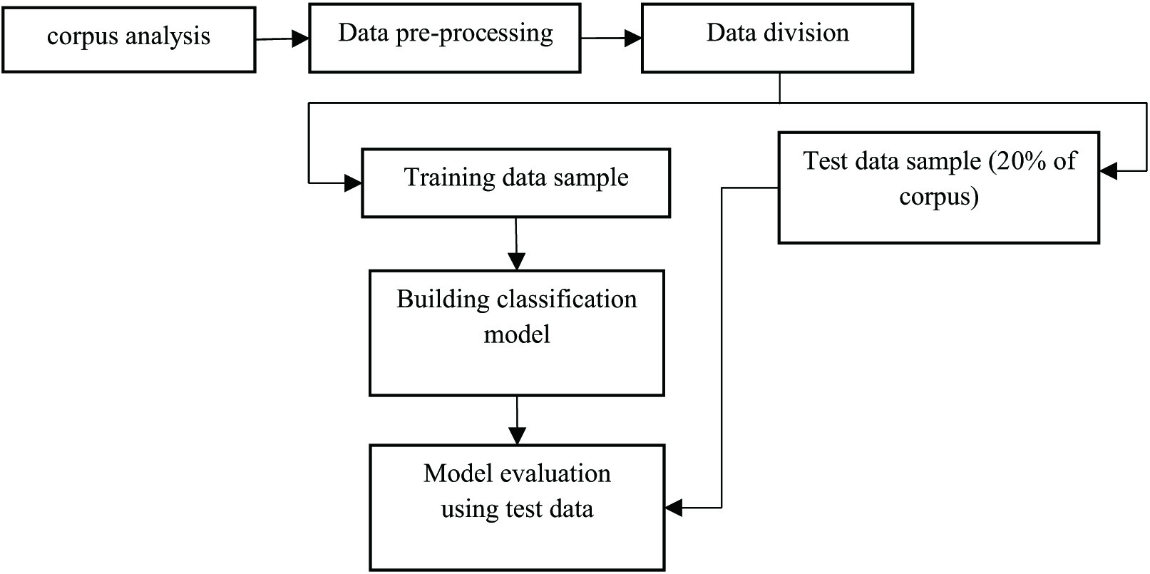 Fig. 2. Model designing and evaluation using deep learning.
Preprocessing as shown in Fig. 2 is a very important task, since clean and normalized data lead to accurate extraction of features else wrong extracted features could lead to an inaccurate trained model.
Besides, various algorithms and methods are there to build the classification model for cancer diagnosis, but we will experiment with the autoencoders to get the accurate result in comparison to other models. Autoencoders are the algorithm that uses backpropagation to set the target values to be equal to the inputs available, and it is an unsupervised machine learning algorithm.
The basic building blocks of an autoencoder are the input layer (the first layer), the concealed layer (the yellow layer), and the output layer (the final layer). For the network to succeed, the input and output layers must be identical. Feature extraction, or the process of finding elements that influence the result, makes advantage of the hidden layers. The transition from the topmost layer to the bottommost layer is described by encoding. Decoding is a term used to describe the change from the hidden layer to the output layer. Because of how they encode and decode data, autoencoders are special. The concealed bottleneck layer, often known as the yellow layer, is occasionally used. Keep in mind that there are more hidden layers than input/output layers. This is necessary if one’s data has more characteristics than is typical. The main issue with this is that the inputs might be processed without being altered; hence, no true feature extraction would take place. The basic structure of autoencoders is to mainly constrain the total available modes in the model’s hidden layer and constrain the total information that would flow via the network. By limiting the network as per reconstruction error, the model would understand the very crucial attribute of inputted data and will help us to redevelop the original input from the encoded one [25–28]. Overall, we can say that encoding will be learned and explain the attributes of inputted data. The basic structure of autoencoders is to mainly constrain the total available modes in the model’s hidden layer and constrain the total information that would flow via the network. By limiting the network as per reconstruction error, the model would understand the crucial attribute of inputted data and help us redevelop the original input from the encoded one. Overall, we can say that encoding will be learned and explain the attributes of inputted data.
B.PROPOSED METHODOLOGY IMPLEMENTATION
This work will study the various deep learning algorithms like ANN, CNN, and RBM to witness whether our autoencoder accuracy is better and implement the proposed methodology and will graphically present the model’s accuracy at the end of the proposed new methodology or algorithm for rectal cancer’s patients.
You may think of each perceptron (or neuron) as a single logistic regression. In an ANN, several neurons and perceptrons are joined together at each layer. ANN is sometimes known as a “feed-forward neural network,” since inputs are always processed in the forward manner. An ANN consists of three layers: output, hidden, and input. The input layer takes in input, the hidden layer processes it, and the output layer produces the result. Every layer essentially tries to learn certain weights. A synthetic neural network has the ability to learn any nonlinear function. Therefore, the term “universal function approximators” is frequently used to refer to these networks. The weights that ANNs can learn can be used to map any input to any output.
CNNs have recently been the deep learning community’s obsession. Although there are many situations and applications where these CNN models are used, image and video processing projects are where they are most commonly used. CNNs are built on the kernels, sometimes referred to as filters. Kernels are used with the convolution approach to extract the crucial data from the input. CNN makes no mention of the filters’ automated learning process. These filters allow the appropriate and necessary properties to be derived from the incoming data. CNN analyzes images to glean spatial information. Spatial features pertain to how pixels are arranged and interact within an image. They help us recognize objects clearly, locate them, and comprehend their locations.
RBM-type ANNs are used for unsupervised learning. A probability distribution may be found from a collection of input data via this form of generative model. The two layers of this specific neural network are a visible layer and a hidden layer of neurons. The visible layer serves as a representation of the input data, while the hidden layer serves as a representation of the learnt attributes. Because connections between neurons in the same layer are not allowed, the RBM is referred regarded as being “restricted.” So each neuron in the visible layer is only connected to neurons in the hidden layer, and vice versa. The RBM could learn a compressed version by decreasing the dimensionality of the input. The network changes the weights of the connections between neurons during training to maximize the probability of the training data. Once trained, the RBM may be used to produce fresh samples based on the learned probability distribution.
- •Restricted Boltzmann Machine (RBM)
RBM modeling technique uses probability to make predictions about an unsupervised model [29,30]. The construction of an RBM model is shown in Fig. 3. Each visible node takes a low-level attribute from the item in the corpus that has to be trained. When x is multiplied by a weight and added to a bias (b) in this input, an activation function is created that determines the output or strength of the node receiving or passing through it (Figs. 4, 5).
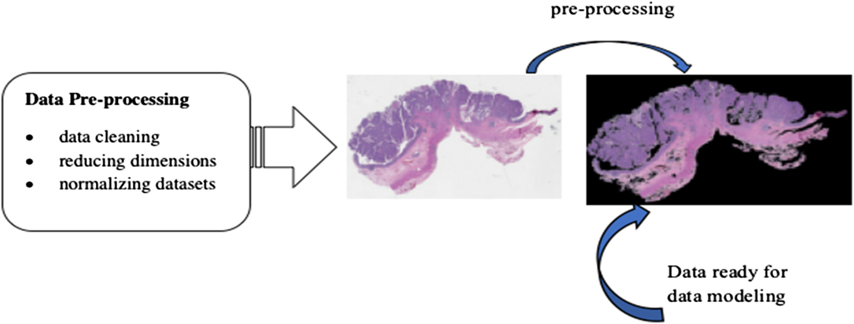 Fig. 3. Dataset preprocessing.
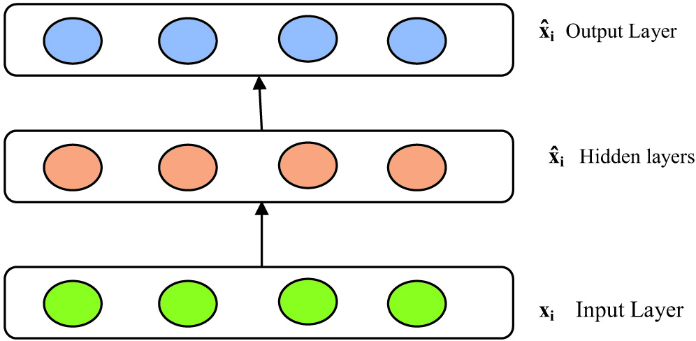 Fig. 4. Under complete autoencoders reconstruction of inputted values.
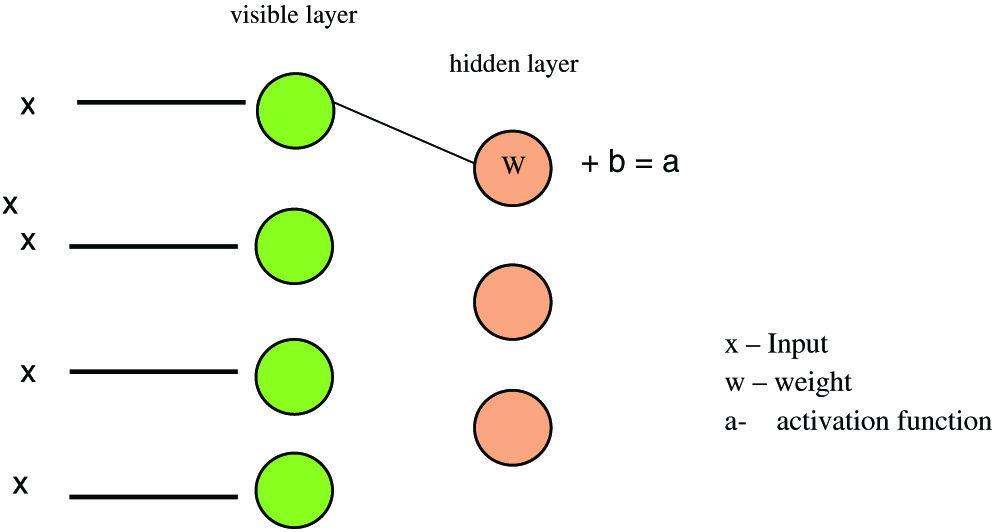 Fig. 5. RBM model representation.
For training RBM model sampling and divergence are done, and it is the main step that leads to the pupation of the weight matrix, so V0 and Vt input vectors are used to calculate activation probabilities for hidden layer h0 and ht, and the updated matrix is equal to the difference between the outer output of activation probabilities with input vectors:
Gradient ascent is used to measure the new weights:
- •Recurrent Neural Networks
This deep learning method has a looping scenario, which means information gets stored in the network nodes and uses the pattern or reasoning of previous experiences to get information about upcoming events. This model works better in the sequential form of inputs and helps to perform complicated tasks (Fig. 6).
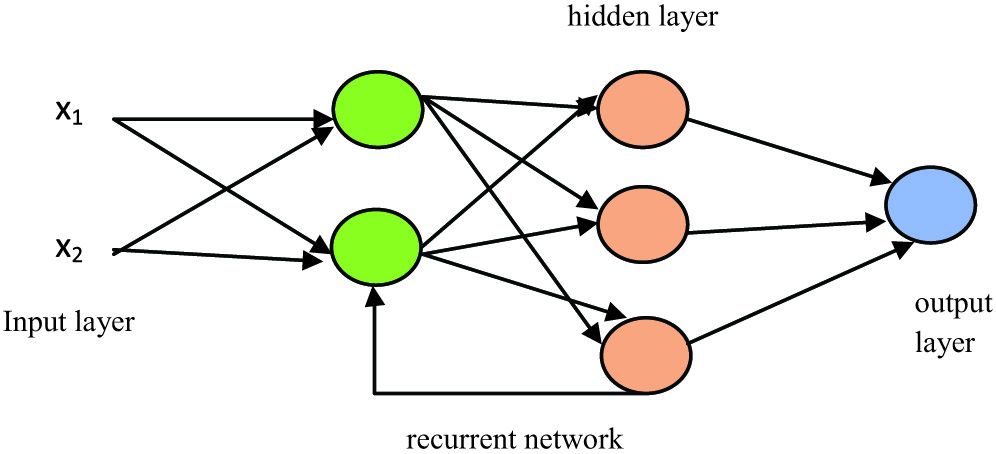 Fig. 6. RNN model representation.
As shown in Fig. 3, any processing done in the hidden layer then backtracks to the previous reasoning and leads to the processing in a hidden layer in looping and will provide us the output. However, the main disadvantage is that it is slower in processing and has a gradient problem while training the model.
- •Convolutional Neural Networks (CNNs)
CNNs can operate large volumes of input values. In this every layer, quest for patterns within the data or corpus is available [28]. CNN includes the construction of convolution, pooling layers, and then followed by fully connected layers, and patterns are learned instantly through backpropagation as shown in Fig. 7.
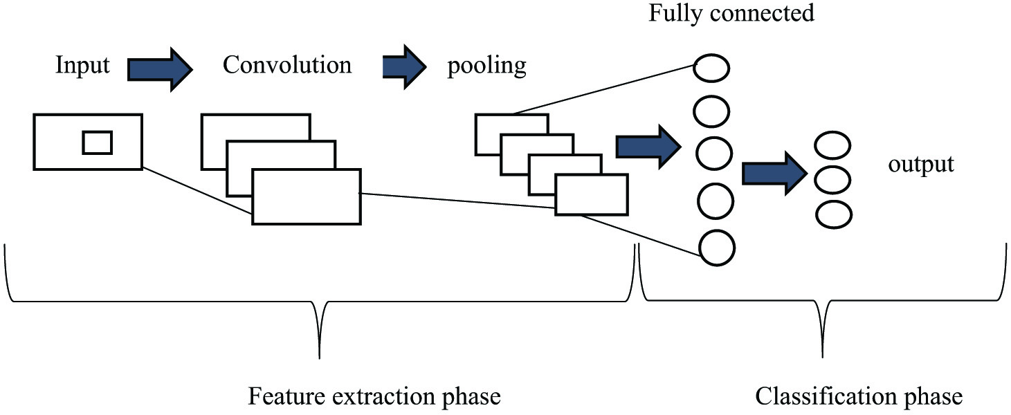 Fig. 7. CNN model representation.
For the purpose of patient survival, the convolutional 1-D model was applied in our experimental investigation to identify cancer [31–33]. A deep neural network may be trained to classify sequence data using a 1D CNN. Sliding convolutional filters are applied to 1-D input to teach features to a 1-D convolutional layer. Convolutional layers can process information more quickly than recurrent layers, since they can do so in a single operation. Recurrent layers, however, are required to cycle over the input’s time steps. By using the root means square propagation approach, the model is optimized. The inner layers take the input as a matrix and use different filters, and the pooling layer is used to pool the output.
- •Variational Autoencoders (VAE) with a deep learning algorithm
VAEs are used to get the inference and generative, and basically, we encode and decode the corpus as shown in Fig. 8. The main difference between the autoencoders and VAEs is that autoencoders are deterministic in approach, and the latter one is a probabilistic one. Besides, VAE is an autoencoder; those are trained to avoid the overfitting problem and witness that latent space would have accurate properties that will enable generative process and encoding, decoding is done at latent space instead of at a single point [34].
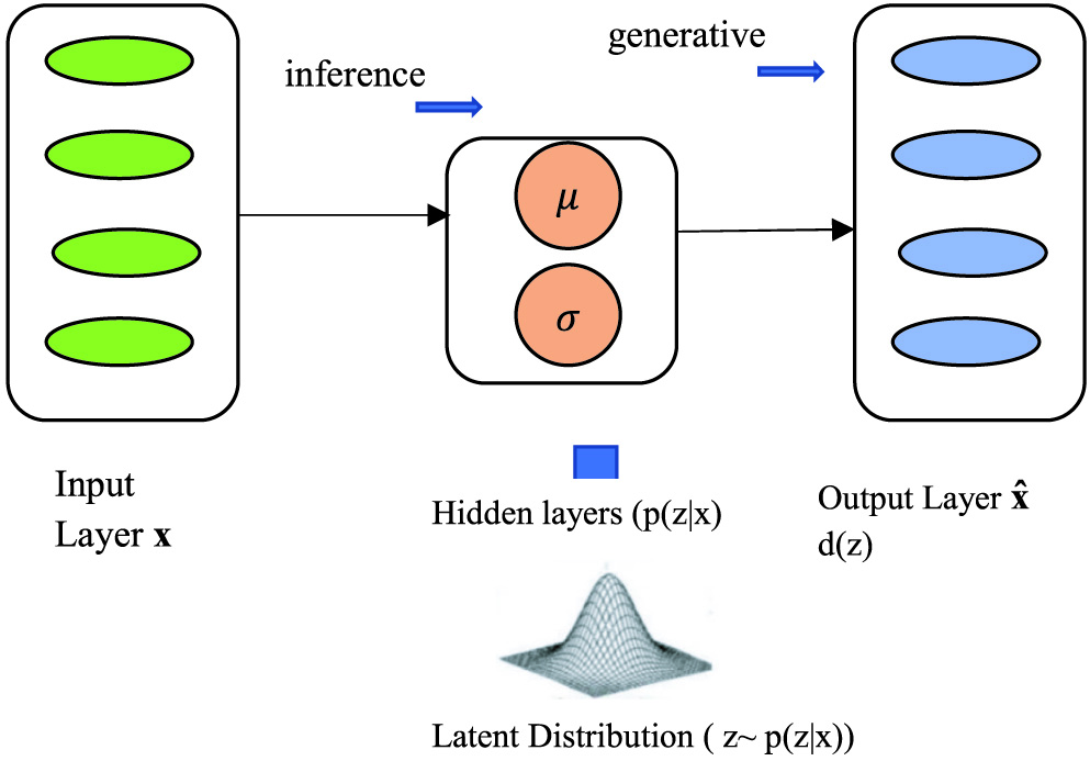 Fig. 8. Variational autoencoders (VAEs) model representation.
In VAE, for calculating loss function, two terms are their reconstruction term and regularization term, and these make the encoding–decoding process efficient and latent space regular, respectively:
In the hidden layer, the (p(z|x) can be calculated as:
It is quite difficult to calculate the value of p(x) mathematically in the above-given formula, so we use the variational inference to calculate the same. This decoder network is used to develop the generative model that could be capable enough to create new data similar to the training set data. In this sampling, the prior distribution is done specifically, and we are supposed to follow a unit Gaussian distribution.
IV.RESULTS AND DISCUSSION
Experiments are done to get the model with high accuracy which is measured through various parameters like true positive rate, ROC curve, and accuracy scores. Finally, in the end, we calculate the accuracy score for every model. The ROC curve represents the performance of a classification model at each classification threshold on a graph. This graph displays these two measurements, the true positive rate and false positive rate. True positive rate (TPR) vs. False positive rate (FPR) is displayed on a ROC curve at various levels. Both false positives and true positives increase as the classification criterion is reduced because more objects are labeled as positive. The points on a ROC curve might be produced by continually analyzing a logistic regression model with different classification criteria, but that would be ineffective. We may, happily, obtain this knowledge using the rapid sorting approach known as area under the ROC curve (AUC). AUC measures the total effectiveness of all possible categorization criteria.
A.MODEL EVALUATION BASED ON THE TRUE POSITIVE RATE
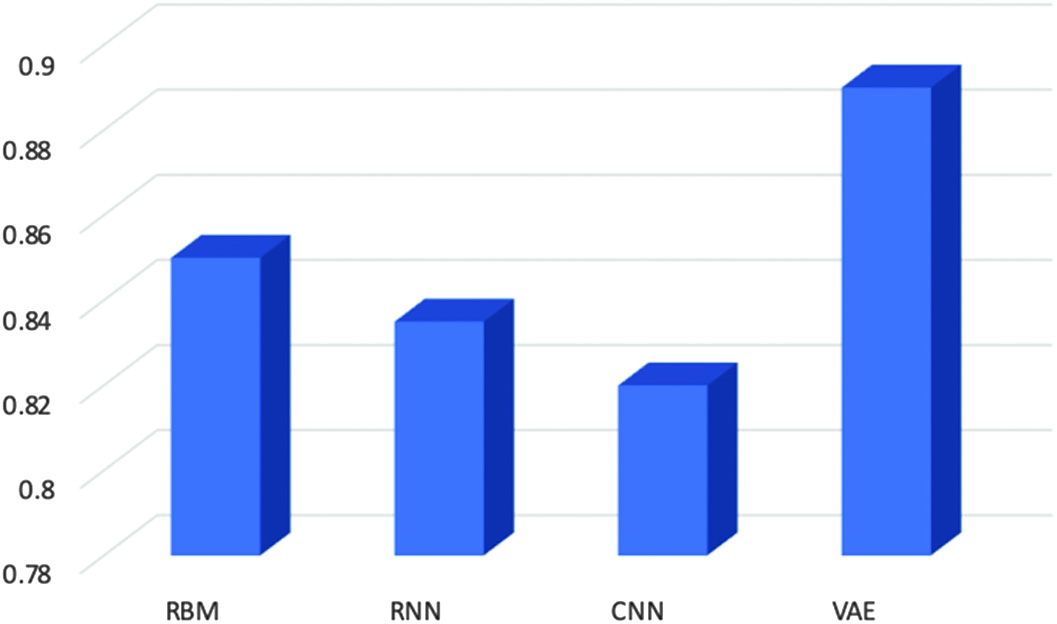
The ratio of true positives (TP) to total positive counts (true positive + false negative) is known as the true positive rate, often referred to as “sensitivity” or “recall.” We can also use precision for model evaluation, but precision alone is not enough to produce correct positive prediction, so an advanced version of precision is used named sensitivity. Two parameters are required to calculate the true positive rate function: predicted target labels and corrected target labels (Fig. 9).
B.CLASSIFICATION MODEL EVALUATION USING RECEIVER OPERATOR CHARACTERISTIC CURVE
According to our calculations, the attained AUC for the variable autoencoders is 0.94, as shown in Fig. 10. It is also the highest of all. A higher AUC score indicates that the model performs better than all other models combined. There is a higher chance that the model can distinguish positive values from the negative class value when 0.5 < scores < 1. So, all models are capable enough to diagnose cancer, but the best one is with a higher value which is VAEs.
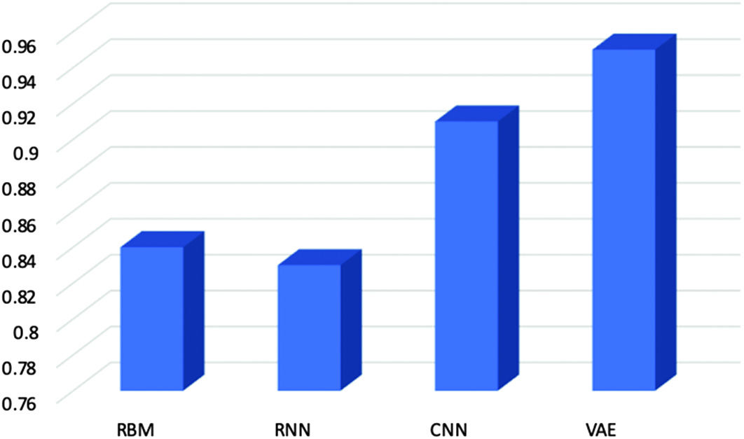 Fig. 10. Area under receiver operator characteristic curve’s score for evaluating models.
C.CLASSIFICATION MODEL ACCURACY
The best accuracy model is achieved by the VAEs among all other deep learning models and accuracy is calculated by the ratio of the correct achieved model divided by total predictions:
In this, we have discovered that the VAE model outperforms other prediction models as shown in Fig. 11. A fine-tuning strategy is used to specify and optimize all of the model’s parameters. Additionally, rather than only reconstructing the input values according to extracted characteristics, the VAE model is trained to learn abstract attributes. The simulation findings demonstrated that rectal cancer patient estimates may be made using prediction models. It has been demonstrated that variational deep encoders are extremely accurate, with a cancer prediction accuracy of 94% and an AUC accuracy of 95% (Fig. 12).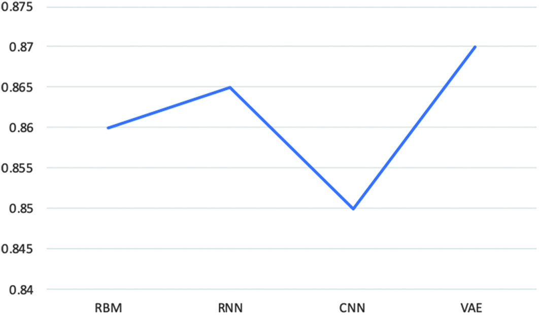 Fig. 11. Accuracy score for evaluating classification models.
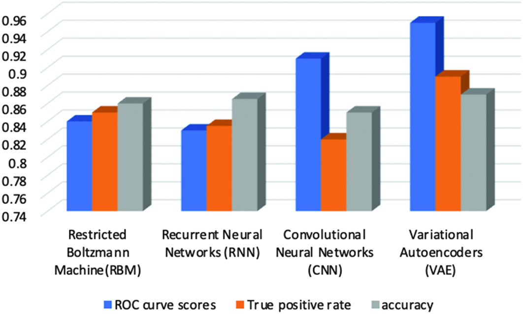 Fig. 12. Graphical representation highlighting the best performance of autoencoders model.
V.CONCLUSION
One kind of cancer that starts in the large intestine is rectal cancer. Although making an early cancer diagnosis is extremely challenging, a lot of study has been done in this area. Early diagnosis and faultless execution of curative operations are considered two of the most effective methods for treating cancer. This is especially true for receiving proper information regarding rectal cancer at an early stage. In this study, we examined rectal cancer data from the CDAS program to create reliable rectal cancer patient survival prediction models. In order to undertake a comparative study, we have also experimented with a variety of deep learning models. After careful consideration, we conclude that the VAE is the model that best achieves appropriate prediction performance, as evidenced by the scores for the AUC true positive rate, and accuracy. Future research can use the outcomes of the autoencoders developed through the interplay of various cancer datatypes to forecast and characterize patient groups and survival profiles.