I.INTRODUCTION
Accessing the Internet for communication, teamwork, email, e-banking, e-commerce, e-learning, e-governance, and other productivities is almost impossible unless users interact with a specific website. However, because phishing websites resemble benign and not all online users have adequate insights and skills on how to discriminate between benign and phishing websites, they are duped into disclosing valuable information such as login credentials, ATM passcode, and details of credit card, bank account, and Social Security Number (SNN) to the carefully crafted phishing sites. Phishing attack risks user privacy, and users who visit phishing websites are becoming vulnerable to harmful software attacks like ransomware [1], which locks the entire computer system or its contents until the requested ransom is paid. The phishing website attack success may result in losses in finances, productivity, reputability, credibility, continuity, and damage to national security [2]. Therefore, the development of cyberattack detection systems is essential for the security of sensitive and personal data, data exchanges, and online transactions [3].
The major source of phishing attacks is emails online users receive and website users visit on daily basis [4], and online user inadequacy is one of the main success factors for such attacks. The success of the user education approach largely depends on how effectively it can teach online users about the different tactics followed by the cybercriminals. Having a clear understanding of phishing attack tactics helps them to correctly differentiate between legitimate websites/emails and phishing websites/emails [5]. More efficient and automatic phishing detection systems are needed because we cannot only rely on people to recognize it [6].
A recent study [3] stated that most cyberattack detection and prevention techniques employed in current systems are incapable of dealing the complexity and dynamic nature of cyberattacks. To address these concerns, it is vital to employ adaptive AI-based techniques like machine learning (ML) and deep learning (DL) by considering enhanced detection, low false alarms, and reasonable costs of computation [3]. As per [7], DL is a subset of ML techniques based on multilayered neural networks. DL is not necessarily outperforming the ML because when few features are included in the training data, ML can yield results that are comparable to those of DL. Despite DL has benefits over ML in terms of handling both large and complicated data, it still needs more processing resources and has more difficult-to-interpret results [7].
A.THE FOLLOWINGS ARE AMONG THE RATIONALES FOR UNDERTAKING THIS STUDY
Despite significant efforts made by the scientific community to address them, the alarming rate increase of unique phishing website attacks continues unabated. This issue highlights the dynamic nature of phishing attacks and the defects of the existing anti-phishing solutions. Recent statistics on phishing activity from the Anti-Phishing Working Group (APWG) exhibit that there are more and more targeted unique phishing website attacks. As depicted in Fig. 1, as depicted in Figs. 1 and 2, APWG was able to record 1,025,968 unique phishing websites in the quarter one of 2022 [7], 1,097,811 in the quarter two of 2022 [8], 1,270,883 in the quarter three of 2022 [9], and 1,350,037 in the quarter four of 2022 [10].
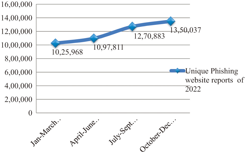 Fig. 1. The quarterly distinct phishing website attack reports of 2022 by APWG [7–10].
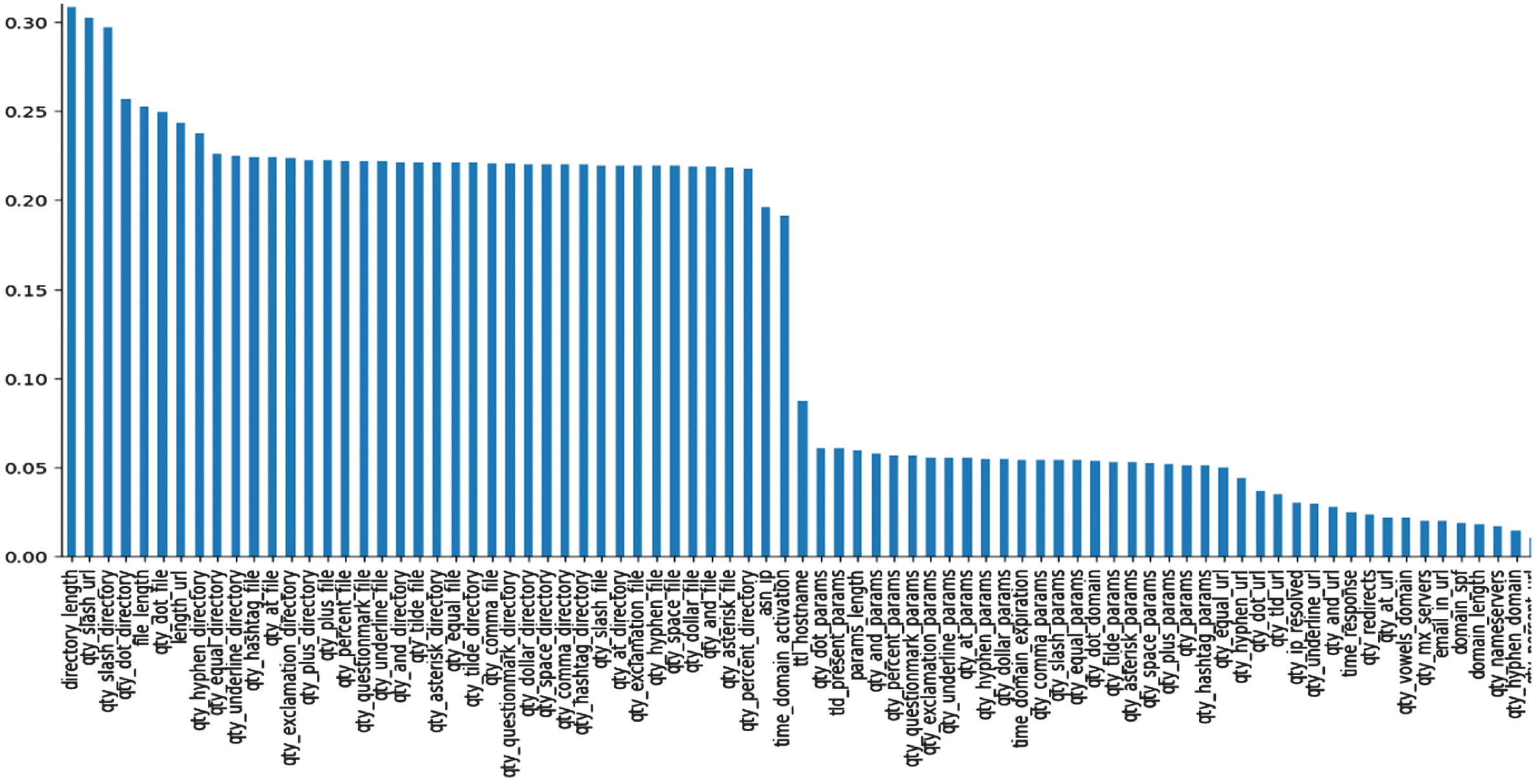 Fig. 2. The top 80 phishing website predictive features selected from DS-2 after the MI technique was applied to the CATB classifier.
Despite a lot of studies employing ML and DL for phishing website detection [11,12], in phishing website detection there is no common consensus reached on which classifier (ML or DL) is more desirable when the objective is to enhance detection accuracy while cutting down the computational time.
For example, recent studies [13–19] have all used ML and DL algorithms to detect phishing websites. As per the authors’ comparative analysis results, the highest accuracy was attained by random forest (RF) in [13,14], the support vector machine (SVM) in [16], naïve bayes (NB) in [19], convolutional neural network (CNN) in [17], eXtreme gradient boosting (XG)-Boost in [15], and the logistic regression (LR) in [18].
There are hundreds of research works focused on ML applications in cybersecurity in general, phishing website detection in particular; however, one of the big confusions on what actually works best and impairs the real deployments of ML is that most researchers either intentionally or unintentionally fail to demonstrate the entire information needed to reproduce their experimental findings [20]. Some studies exhibit that DL approaches outperform “traditional” ML approaches, despite the opposite results claimed by another study that used exactly the same experimental setting [20].
There is still a lack of common agreement among academics on the suitability of website features for phishing attack detection [12]. For example, for phishing website detection there are studies that excluded domain-based, and page ranks features [21–25], and concentrated mostly on URL-based features [1,26] because URL-based features are more suitable for run-time analysis, and some studies do not include web content features because content-based features are not available for extraction as a result of phishing websites short lifespan [12]. However, the study [27] challenged the aforementioned studies claim, stating that obtaining domain name system (DNS) and page-rank features was computationally faster than obtaining web-content-based features and that more web-content-based features could be obtained with the aid of a “Python-based HTML DOM tree Parser” despite the presence of dead links, and as per study [28], the network delay at the time of detecting phishing websites could be remedied by having access to fast Internet connectivity and other methods.
The contributions of our work are presented as follows.
- •Rigorously reviewed recent research works, identified core gaps, and attempted to address those gaps using experimental-based pieces of evidence.
- •Used the top-performed ML and DL algorithms identified from a recent literature survey [11,12] such as RF, gradient boost (GB), LR, multilayer perceptron (MLP), and deep neural network (DNN). Introduced cat-boost (CATB) classifier in this work due to it being the latest version of the ML algorithm but not considered by the reviewed studies.
- •Each classifier experimented with three trustworthy datasets to look for performance consistency and scalability across all datasets. This approach was overlooked by most of the reviewed studies
- •Examined the role of relevant feature selection techniques on each classifier’s performance and evaluated each classifier using accuracy, F1-score, area under receiver operating characteristic curve (AUC-ROC), false negative rate (FNR), false positive rate (FPR), and train-test computational time as core model evaluation metrics.
- •Our study results were compared with other study results that used the same dataset.
In short, the study attempted to address the following research questions (RQ).
- RQ#1: What are the optimal model parameters to use with the CATB, GB, RF, MLP, and DNN classifiers?
- RQ#2: Does employing the feature selection techniques enhance accuracy while cutting down on each classifier’s train-test computational time?
- RQ#3: Which classifier among the CATB, GB, RF, MLP, and DNN exhibits superior and consistent accuracy with acceptable train-test computational time across three distinct datasets?
II.RELATED WORKS
The reviewed related research works are presented as follows.
The RF, LR, decision tree (DT), SVM, and Naïve–Bayes classifiers were employed by [27] for phishing website detection and the RF attained the highest accuracy of 96.83%. The RF, NB, CNN, and LTSM were employed by [19], and the NB classifier attained the highest accuracy of 96.01%. The study [25] employed GB, RF, and ANN for phishing website detection and GB attained the highest accuracy of 96.4%, despite GB not being tested on varied nature datasets to ensure performance consistency, not tested on the domain-based and page rank-based features, and not subjected to the run-time analysis despite being supposed to be assessed to ensure its suitability for real-time execution.
The RF, NB, C.45, JRiP, and PART classifiers experimented with the hybrid ensemble feature selection (HEFS) technique by [22] and the RF demonstrated the highest accuracy of 94.6%. The study did not include DL algorithms and did not include features from domain and page rank. Despite not being tested on domain and web content features, the RF classifier employed in [23] for phishing website detection and attained the greatest accuracy of 99.57%. Similarly, despite not having been tested on features based on web content, the RF classifier used by [1,26] achieved the greatest accuracy of 98.03% and 99.3%, respectively. RF achieved the highest accuracy in the investigation, with scores of 94.6%, 99.8%, and 99.09%, despite not being tested on the domain and page-based features [21,22,29], respectively.
The recent [30] employed DNN for phishing website detection and attained the highest accuracy of 96.25% despite not being tested on varied nature datasets to ensure performance consistency and not being subjected to the run-time analysis despite it being supposed to be assessed to ensure its suitability for real-time execution. MLP was employed by [31,32] for phishing website detection, and MLP demonstrated the highest accuracy of 98.5% and 93%, respectively, despite not being tested on varied nature datasets to ensure performance consistency and not being subjected to the run-time analysis despite being supposed to be assessed to ensure its suitability for real-time execution.
The study [33] employed CNN for phishing website detection and attained the highest accuracy of 94.8%. The MLP, CNN, KNN, and SVM classifiers were employed by [17] for phishing website detection and CNN attained the highest accuracy of 97.94% despite not being tested on varied nature datasets to ensure performance consistency and not subjected to the run-time analysis despite being supposed to be assessed to ensure its suitability for real-time execution.
Each of the reviewed studies used a single dataset to train and test the ML and DL models and did not use the CATB classifier. Most of the reviewed studies did not incorporate domain and page rank-based features for phishing website detection, did not conduct model computational time, and did not reveal each parameter used for ML and DL algorithms. Our study is an attempt to fill the aforementioned gaps.
III.METHODOLOGY
This section presents brief details of dataset sources, data preprocessing, informative feature selection techniques, cross-validation methods, implemented ML and DL algorithms, implementation tools, and model evaluation metrics used in experiments.
A.DATASET SOURCES AND DATA PREPROCESSING
As shown in Table I, the study used three recent and distinct trustworthy public datasets to train and test each classifier. DS-1 represents Dataset 1, DS-2 represents Dataset 2, and DS-3 represents Dataset 3. We did not find any missing values in each dataset.
| Dataset name | # of records | # of attributes/features | Website features coverage | Label | Dataset sources |
|---|---|---|---|---|---|
| DS-1 | 11,430 | 87 | URL, domain, web content, and page rank | 1 → phish and | Created by [ |
| DS-2 | 58,645 | 111 | URL, domain, and page rank | 1 → phish and 0 → benign | Created by [ |
| DS-3 | 10,000 | 48 | URL and web content | 1 → phish and 0 → benign | Created by [ |
In order to create DS-1, the study [27] gathered benign website datasets from Yandex and Alexa, as well as phishing website datasets from open-phish and phish-tank repositories.
To create DS-2, the study [34] gathered benign website datasets from Alexa and phishing website datasets from phish-tank repositories. Each dataset feature was extracted using Python scripts that contain a predefined parsing rule.
To create DS-3, the study [22] gathered benign website datasets from Alexa and the Common Crawl and phishing website datasets from open-phish and phish-tank repositories.
Each DS-1, DS-2, and DS-3 feature has been scaled and centered by removing the mean and dividing it by the standard deviation to have data with a mean of 0 and a standard deviation of 1. The standard scalar formula can be written as follows.
Standard scalar = N-m (N)/ S (N),
where N represents the training sample, m (N) represents the mean of the training samples, and S (N) represents the standard deviation of the training samples.
Because the model will favor the classes that are in the majority, using an unbalanced dataset may result in biased model findings. To address these concerns, the study used a prominent dataset balancing strategy, Synthetic Minority Over-sampling Technique (SMOTE), to modify the uneven dataset ratio of DS-2 from 52%:48% to 50%:50%.
B.INFORMATIVE FEATURE SELECTION TECHNIQUES
When utilizing a feature selection strategy, the fundamental assumption is that the dataset contains a large number of features that are either redundant or irrelevant and can be deleted with little to no information loss. Irrelevant features lack any information that is valuable in relation to the target variable, whereas redundant features have information that is duplicated in other features. In most cases, feature selection serves as a filter, eliminating features that would be redundant with already existing features. Preventing overfitting of predictive models, accelerating computation, and enhancing the results’ interpretability are all benefits of optimal feature selection [35]. Taking into the aforementioned benefits, we employed two popular filter-based feature selection techniques, namely ANOVA-F-test-based univariate feature selection (UFS) and mutual information (MI).
ANOVA-F-test-based UFS treats each feature independently and chooses features while taking into account the randomness and normal distribution of datasets. It chooses feature subsets that have a strong relationship with the target variable. By using statistical tests, the ANOVA-F-test determines whether the means of different variables are significantly varied, that is, categorically dependent or independent. The F-test value is used as a statistical measure to assess the significance of the results. If the variance of the features is equal or the statistical significance (P-value <0.05) is not met, the features will not be included in the dataset [36].
Mutual information (MI) is used to measure the stochastic dependency or shared information between discrete random variables. MI adopts heuristic greedy algorithms to distinguish between the highly relevant and least redundant features at each step [35]. The MI value is set to zero when X and Y are statistically independent, indicating that no information has to be exchanged between them [37]. According to Sulaiman and Labadin [37], unlike correlation-based feature selection, MI is a common option for effective feature selection since it considers both linear and nonlinear relationships between two random variables and is highly robust when the variables are noisy or nonlinearly associated with the target variable [35]. MI is originated from information theory and highly related to the entropy concept, employed to lessen uncertainty. If Y is dependent on X, X’s knowledge reduces Y’s uncertainty [35,37].
C.CROSS-VALIDATION METHODS
The model is said to be effective when it can adjust to new or unforeseen data and yield accurate predictions. One of the methods frequently employed to evaluate the performance of an ML model on unobserved data is holdout cross-validation. In this work, each classifier was trained and tested using 80%–20% dataset splits. The 80%–20% dataset split was a commonly used
D.IMPLEMENTED ML and DL ALGORITHMS
In this study, five ML and DL algorithms namely RF, GB, CATB, MLP, and DNN were employed for phishing website detection. Brief details of each algorithm are presented as follows.
RF classifier: RF is the most frequently used ML algorithm for phishing website detection. When compared to other classifiers, RF attained superior accuracy in 17 out of 30 rigorously reviewed studies in terms of detecting phishing websites [12]. RF is a bagging ensemble method; it follows a divide and conquers strategy [38], and each predictor tree uses randomly assigned values and a vote from each decision tree will be taken for the final classification result, and it is robust, highly accurate, and do not suffer from overfitting issues [38]. The study used Max_depth, N_estimators, and Random_state to look for the optimal parameter setting of the RF classifier, and the theoretical definitions of these parameters can accessed from [39].
GB classifier: GB is a boosting ensemble model of decision trees and follows a sequential approach for training [40]. GB is supported by strong theoretical results that describe how strong predictors can be constructed by the iterative combination of base predictors (weaker models) via a greedy procedure that belongs to gradient descent in a function space [41]. GB is an efficient ML algorithm that has been employed in diverse fields, such as environmental variable prediction, weather forecasting, web searching, diabetes prediction, driving style recognition [42], and phishing website detection [12] with promising results. The study used Max_depth, N_estimators, Learning_rate, and Random_state to look for the optimal parameter setting of the GB classifier, and the theoretical definitions of these parameters can accessed from [39].
CATB classifier: CATB is a recent and advanced version of the gradient boost decision tree (GBDT) method and devised by Dorogush, et al. in 2018 [41]. CATB is an open source, a member of the family of GB ML ensemble techniques. CATB introduced two major innovations namely ordered target statistics (OTS) for automatic encoding of categorical variables when one hot encoding is not used by CATB [29] and ordered boosting tree (OBT) to avoid target leakage or prediction shift caused by the expected value of encoded variable by applying random permutations of the training dataset to reduce variance and increase the robustness of the learning algorithm [29,41,43]. OBT is less prone to overfitting, is balanced, and allows significant speedup of execution at testing time [29,43]. However, one must be careful in setting the CATB maximum tree depth to balance the trade-off between memory and speed because for every unit of increase in the maximum tree depth, the amount of memory CATB will use may increase by a factor of two times the number of trees in an ensemble [29]. The study used Max_depth, Iterations, Learning_rate, and Random_state to look for the optimal parameter setting of the CATB classifier, and the theoretical definitions of these parameters can accessed from [39].
MLP classifier: MLP is the most successful and commonly used feed and forward neural network and is a category of supervised DL algorithm [17,32]. It was applied in diverse fields, including image compression, autonomous vehicle control, speech recognition, medical diagnosis, financial data prediction, and newly discovered applications, as per [17]. Optimizing the MLP classifier performance requires the adjustment of the layers network, as per [17]. MLP contains multiple layers with a nonlinear activation function and uses backpropagation for learning [32]. The following hyperparameters were used to optimize the MLP classifier performance. The study used appropriate activation function, hidden layer sizes, optimizer or solver, batch size, Max_iter, and Random_state to look for the optimal parameter setting of the MLP classifier
DNN classifier: DNN is an algorithm inspired by the works of the human brain. It incorporates more than one hidden layer, as per [30]. Increasing the number of input features and the size of the parameter can affect the computing speed of the DNN classifier. The DNN model can be learned using the back-propagation learning process, as per [11]. DNN algorithm is very analogous to the traditional MLP algorithm; however, the amount of hidden layers for DNN is higher than that of a typical MLP-based model. The model’s performance is affected by the suitable selection of these hyperparameters as per [11]. Due to the aforementioned reasons, the following hyperparameters were used for DNN to optimize its performance as shown in Table II.
Table II. Description of DNN model parameters
| DNN parameters | Conceptual details |
|---|---|
| Activation function | We used the ReLU activation function for the hidden layers and the sigmoid function for the output layer. |
| Batch normalization | We used the batch normalization function to standardize input data for each layer, reduce the data by adjusting and scaling the activation functions, minimize the loss function, and reduce undesirable shifts to yield more reliable model training. It is used to enhance the accuracy, stability, and speed of the DNN algorithm [ |
| Dense layer | We used the dense layer to specify the number of hidden layer sizes and the number of nodes/units/neurons in each layer. To look for the optimal parameter values, we checked different numbers of neurons like 512, 256, 128, 64, 32, and others. |
| Dropout | We used dropout as a regularization technique for ignoring unwanted hidden layer nodes to avoid overfitting [ |
| Output layer neuron | We used a single neuron for the output layer to yield either phishing or benign website. |
| Loss function | The network is compiled by a loss function which is responsible for specifying what model evaluation metric to use and used “binary_crossentropy” to calculate the train-validation loss of the DNN [ |
| Batch_size | We used this parameter to determine data samples to be considered prior to weight adjustment [ |
| Epoch | We used this parameter to determine the number of iterations/passes throughout the process of training data samples and used to control model overfitting. |
| Optimizer | We used the Adam optimizer to search the optimal weights for the DNN and MLP algorithms [ |
E.IMPLEMENTATION TOOLS
Each experiment was conducted using a Google co-lab cloud environment and Python code. We used Pandas, NumPy, and Matplotlib libraries for data handling, analysis, and visualizations. We used the skit-learn library to implement classifiers like CATB, GB, RF, and MLP. We used the Keras library run on tensor flow to implement the DNN algorithm.
F.MODEL EVALUATION METRICS
The study used accuracy, F1-score, AUC-ROC, FNR, FPR, and train-test computational time as core model evaluation metrics. True positive rate (TPR) is the number of phishing websites that have been correctly classified as phishing. True negative rate (TNR) is the number of benign websites that have been appropriately identified as benign. The FPR indicates the number of benign websites that have been wrongly branded as phishing websites, and the FPR prevents Internet users from accessing authentic websites. FNR shows the amount of phishing websites that have been incorrectly categorized as benign websites, and in this case, the FNR permits Internet users to visit phishing websites, which is risky. Hence, minimizing or avoiding both FPR and FNR is key to combating phishing website attacks.
IV.RESULT AND DISCUSSIONS
The experimental results were grouped under the RQ as follows to make the presentations simpler to understand.
- RQ#1: What are the optimal model parameters to use with the CATB, GB, RF, MLP, and DNN classifiers?
As stated in the recent study [20], most researchers either intentionally or unintentionally fail to demonstrate the entire information needed to reproduce their experimental findings and impairs the real deployments of ML. Some studies exhibit that DL approaches outperform “traditional” ML approaches, despite the opposite results claimed by another study that used exactly the same experimental setting [20].
To address these concerns, our study showed how each model parameter was employed in detail to facilitate the replication of research results as shown in Table III. When employing DS-1 and DS-2, each classifier was tested with the UFS and MI feature selection techniques, while DS-3 was tested without the use of the aforementioned feature selection techniques. Table III demonstrates the optimal model hyperparameters after the UFS and MI were applied to DS-1 and DS-2. Table IV demonstrates the optimal model hyperparameters without the application of the UFS and MI techniques to DS-3.
- RQ#2: Doesemploying the feature selection techniques enhance accuracy while cutting down on each classifier’s train-test computational time?
Table III. Each classifier’s optimal parameter values after the UFS and MI techniques applied to DS-1 and DS-2
| Classifiers | Optimal model parameter values for DS-1 | Optimal model parameter values for DS-2 |
|---|---|---|
| CATB +UFS | No. of features: 69 | No. of features: 93 |
| max_depth=5, | max_depth=8, | |
| iterations=350, | iterations=215, | |
| learning_rate=0.1, | learning_rate=0.1, | |
| random_state=0 | random_state=12 | |
| GB +UFS | No. of features: 69 | No. of features: 97 |
| max_depth=5, | max_depth=7, | |
| n_estimators=69, | n_estimators=85, | |
| random_state=3 | random_state=3 | |
| RF +UFS | No. of features: 69 | No. of features: 96 |
| max_depth=10, | max_depth=13, | |
| n_estimators=32, | n_estimators=96, | |
| random_state=12 | random_state=1 | |
| MLP+UFS | No. of features: 47 | No. of features: 95 |
| hidden layer sizes: 115 | hidden layer sizes: 256,128 | |
| activation: relu | activation: relu | |
| Max-iter:4 | Max-iter:4 | |
| solver: Adam | solver: Adam | |
| batch size:20 | batch size:64 | |
| random state: 3 | ||
| DNN+ UFS | input_dim:55 | input_dim:100 |
| BatchNormalization(), | BatchNormalization(), | |
| dense layers: 128,64 | dense layers: 256,128,64 | |
| dropout: 0.03 | dropout: 0.02 | |
| optimizer: Adam | optimizer: Adam | |
| epochs: 6 | epochs: 7 | |
| activations: ‘relu’ for the hidden layers and ‘sigmoid’ for the output layer. | activations: ‘relu’ for the hidden layers and ‘sigmoid’ for the output layer. | |
| batch size: 80 | batch size: 190 | |
| loss: 'binary_crossentropy' | loss: 'binary_crossentropy' | |
| CATB+MI | No. of features: 64 | No. of features: 80 |
| max_depth=5, | max_depth=7, | |
| iterations=348, | iterations=214, | |
| learning_rate=0.1, | learning_rate=0.2, | |
| random_state=3 | random_state=12 | |
| GB+MI | No. of features: 76 | No. of features: 90 |
| max_depth=5, | max_depth=7, | |
| n_estimators=69, | n_estimators=32, | |
| learning_rate=0.1, | learning_rate=0.2, | |
| min_samples_split=6, | ||
| min_samples_leaf=5 | ||
| random_state=3 | random_state=3 | |
| RF+MI | No. of features: 76 | No. of features: 90 |
| max_depth=10, | max_depth=13, | |
| n_estimators=76, | n_estimators=95, | |
| min_samples_split=6, | ||
| min_samples_leaf=5 | ||
| random_state=0 | random_state=2 | |
| MLP+MI | No. of features: 73 | No. of features: 90 |
| hidden layer sizes: 115 | hidden layer sizes: 128,128 | |
| activation: relu | activation: relu | |
| Max-iter:6 | Max-iter:3 | |
| solver: Adam | solver: Adam | |
| batch size:20 | batch size:86 | |
| DNN+MI | input_dim:64 | input_dim:90 |
| BatchNormalization(), | BatchNormalization(), | |
| dense layers: 128,64 | dense layers: 256,128,64 | |
| dropout: 0.002 | dropout: 0.04 | |
| optimizer: Adam | optimizer: Adam | |
| epochs: 7 | epochs: 7 | |
| activations: ‘relu’ for the hidden layers and ‘sigmoid’ for the output layer. | activations: ‘relu’ for the hidden layers and ‘sigmoid’ for the output layer. | |
| batch size: 86 | batch size: 248 | |
| loss: 'binary_crossentropy' | loss: 'binary_crossentropy' |
Table IV. Each classifier’s optimal model hyperparameters without application of the UFS and MI techniques to DS-3
| Classifiers | Optimal model parameter values for DS-3 |
|---|---|
| CATB | max_depth=7, |
| iterations=35, | |
| learning_rate=0.3, | |
| random_state=0 | |
| GB | max_depth=6, |
| n_estimators=45, | |
| random_state=3 | |
| RF | max_depth=11, |
| n_estimators=50, | |
| random_state=12 | |
| MLP | hidden layer sizes: 256,128 |
| activation: relu | |
| Max-iter:4 | |
| solver: Adam | |
| batch size:64 | |
| DNN | BatchNormalization(), |
| dense layers: 128,128 | |
| dropout: 0.01 | |
| optimizer: Adam | |
| epochs: 9 | |
| activations: ‘relu’ for the hidden layers and ‘sigmoid’ for the output layer. | |
| batch size: 64 | |
| loss: 'binary_crossentropy' |
The ML- and DL-based phishing website detection model is deemed successful when it achieves improved detection accuracy, minimal false alarm rates, and affordable computation costs [3]. In this study, results in bold italics were improved performance indicators, those in bold were similar performance indicators, and those in italics were poor performance indicators. Each classifier’s performances are presented as follows.
A.CATB CLASSIFIER PERFORMANCE COMPARISONS ON DS-1, DS-2, and DS-3
As per the UFS technique, 69 of the 87 features in DS-1 and 93 of the 111 features in DS-2 were determined to be statistically significant in the CATB classifier’s ability to detect phishing websites. As per the MI technique, 64 of the 87 features in DS-1 and 80 of the 111 features in DS-2 were determined to be statistically significant in the CATB classifier’s ability to detect phishing websites. All (48) of the DS-3 were subjected to the CATB experiment.
Based on dataset comparisons, DS-3 came out on top with the best CATB accuracy of 98.83%, followed by DS-1 with 97.9% and DS-2 with 95.73% as can be seen in Table V. These experimental results demonstrate that the CATB classifier was the top-performing classifier when applied to all datasets (DS-1, DS-2, and DS-3 in terms of accuracy when compared to the results of GB, RF, DNN, and MLP classifiers.
Table V. CATB classifier performance comparisons on DS-1, DS-2, and DS-3
| Classifier | Dataset type | Accuracy (%) | F1-score (%) | FPR (%) | FNR (%) | Time (sec.) | AUC-ROC | Conf. matrix |
|---|---|---|---|---|---|---|---|---|
| CATB | DS-1 | 97.73 | 97.71 | 2.51 | 2.03 | 7 | 0.9955 | [[112629] |
| [23 1108]] | ||||||||
| DS-2 | 95.48 | 95.71 | 4.87 | 4.2 | 56 | 0.991 | [[5292271] | |
| [259 5907]] | ||||||||
| DS-3 | 98.78 | 98.71 | 1.3 | 1.14 | 8 | 0.9986 | [[106314] | |
| [11 954]] | ||||||||
| CATB + UFS | DS-1 | 8 | [[112827] | |||||
| [21 1110]] | ||||||||
| DS-2 | 4.89 | 82 | [[5291272] | |||||
| [250 5916]] | ||||||||
| CATB + MI | DS-1 | 11 | [[112629] | |||||
| [23 1108]] | ||||||||
| DS-2 | 75 | [[5306257] | ||||||
| [244 5922]] |
Based on dataset comparisons, DS-1 came out on top with the best CATB computational time of 7 seconds, followed by DS-3 at 8 seconds and DS-2 at 56 seconds as can be seen in Table V. When compared to DNN classifier, these experimental results demonstrate that the CATB classifier was the fastest classifier when applied to DS-1 and DS-3, while it was slowest when applied to DS-2. When compared to GB classifier, the CATB classifier was the fastest classifier when applied to DS-1 and DS-2 in terms of computational time, while it was slowest when applied to DS-3.
The experimental findings exhibited in Table V highlight that despite saving storage space as a result of decreasing the number of features, the application of the UFS and MI techniques to the CATB classifier increases computational time. This may be due to the involvement of adjusting optimal model parameters to obtain better accuracy. When we analyze the experimental findings for DS-1 before and after using the UFS and MI techniques, the CATB and UFS combination produced the greatest accuracy (97.9%) and F1-score (97.88%), while the fastest computational time was exhibited when the CATB classifier was applied to DS-1 (refer to Table V). When we analyze the experimental findings for DS-2 before and after using the UFS and MI techniques, the CATB and MI combination produced the greatest accuracy (95.73%) and F1-score (95.94%), while the fastest computational time was exhibited when the CATB classifier was applied to DS-2 (refer to Table V).
B.GB CLASSIFIER PERFORMANCE COMPARISONS ON DS-1, DS-2, and DS-3
As per the UFS technique, 69 of the 87 features in DS-1 and 97 of the 111 features in DS-2 were determined to be statistically significant in the GB classifier’s ability to detect phishing websites. As per the MI technique, 76 of the 87 features in DS-1 and 90 of the 111 features in DS-2 were determined to be statistically significant in the GB classifier’s ability to detect phishing websites. All (48) of the DS-3 were subjected to the GB experiment.
Based on dataset comparisons, DS-3 came out on top with the best GB accuracy of 98.58%, followed by DS-1 with 97.16% and DS-2 with 95.18% as can be seen in Table VI. These experimental results demonstrate that the GB classifier was the second best-performing classifier when applied to all datasets (DS-1, DS-2, and DS-3) in terms of accuracy, while the CATB classifier was the first best performer.
Table VI. GB classifier performance comparisons on DS-1, DS-2, and DS-3
| Classifier | Dataset type | Accuracy (%) | F1-score (%) | FPR (%) | FNR (%) | Time (sec.) | AUC-ROC | Conf. matrix |
|---|---|---|---|---|---|---|---|---|
| GB | DS-1 | 97.03 | 96.99 | 2.94 | 3.01 | 19 | 0.995 | [[112134] |
| [34 1097]] | ||||||||
| DS-2 | 95.12 | 95.39 | 5.77 | 4.07 | 129 | 0.9877 | [[5242321] | |
| [251 5915]] | ||||||||
| DS-3 | 98.58 | 98.5 | 1.39 | 1.45 | 7 | 0.9985 | [[106215] | |
| [14 951]] | ||||||||
| GB + UFS | DS-1 | [[112233] | ||||||
| [32 1099]] | ||||||||
| DS-2 | 4.46 | 185 | [[5273290] | |||||
| [275 5891]] | ||||||||
| GB + MI | DS-1 | [[112134] | ||||||
| [33 1098]] | ||||||||
| DS-2 | 95.38 | 4.46 | 97 | [[5267296] | ||||
| [275 5891]] |
Based on dataset comparisons, DS-3 came out on top with the best GB computational time of 7 seconds, followed by DS-1 at 17 seconds and DS-2 at 97 seconds as can be seen in Table VI. When compared to CATB classifier, the GB classifier was the slowest classifier when applied to DS-1 and DS-2, while it was the fastest classifier when applied to DS-3 due to decreasing computational time by 1 second.
The experimental findings exhibited in Table VI highlight that despite saving storage space as a result of decreasing the number of features, the application of the UFS technique to the GB classifier on DS-2 increases computational time, while the application of the UFS and MI techniques to the GB classifier on DS-2 exhibit the same computational time. When we analyze the experimental findings for DS-1 before and after using the UFS and MI techniques, the GB and UFS combination produced the greatest accuracy (97.16%) and F1-score (97.13%). When we analyze the experimental findings for DS-2 before and after using the UFS and MI techniques, the GB and UFS combination produced the greatest accuracy (95.18%) and F1-score (95.42%), while the fastest computational time was exhibited when the MI technique applied to GB classifier on DS-2 (refer to Table VI).
C.RF CLASSIFIER PERFORMANCE COMPARISONS ON DS-1, DS-2, and DS-3
As per the UFS technique, 69 of the 87 features in DS-1 and 96 of the 111 features in DS-2 were determined to be statistically significant in the RF classifier’s ability to detect phishing websites. As per the MI technique, 76 of the 87 features in DS-1 and 90 of the 111 features in DS-2 were determined to be statistically significant in the RF classifier’s ability to detect phishing websites. All (48) of the DS-3 were subjected to the RF experiment.
Based on dataset comparisons, DS-3 came out on top with the best RF accuracy of 98.24%, followed by DS-1 with 96.63% and DS-2 with 94.21% as can be seen in Table VII. When compared to DNN classifier, these experimental results demonstrate that the RF classifier was the best-performing classifier when applied to DS-3 in terms of accuracy. When compared to MLP classifier, these experimental results demonstrate that the RF classifier was the best-performing classifier when applied to all datasets (DS-1, DS-2, and DS-3) in terms of accuracy.
Table VII. RF classifier performance comparisons on DS-1, DS-2, and DS-3
| Classifier | Dataset type | Accuracy (%) | F1-score (%) | FPR (%) | FNR (%) | Compute time (Sec.) | AUC-ROC | Conf. matrix |
|---|---|---|---|---|---|---|---|---|
| RF | DS-1 | 96.5 | 96.49 | 3.2 | 3.8 | 4 | 0.994 | [[111837] |
| [43 1088]] | ||||||||
| DS-2 | 94.08 | 94.41 | 7.03 | 4.91 | 66 | 0.9861 | [[5172391] | |
| [303 5863]] | ||||||||
| DS-3 | 98.24 | 98.13 | 1.39 | 2.18 | 4 | 0.9984 | [[106215] | |
| [21 944]] | ||||||||
| RF + UFS | DS-1 | 3.98 | [[112134] | |||||
| [45 1086]] | ||||||||
| DS-2 | [[5173390] | |||||||
| [292 5874]] | ||||||||
| RF + MI | DS-1 | 4.07 | 10 | [[112431] | ||||
| [46 1085]] | ||||||||
| DS-2 | 5.12 | 106 | [[5200363] | |||||
| [316 5850]] |
Based on dataset comparisons, DS-1 came out on top with the best RF computational time of 3 seconds, followed by DS-3 at 4 seconds and DS-2 at 65 seconds as can be seen in Table VII. In comparison with the other classifiers, such as CATB and GB, these experimental results demonstrate that the RF classifier was the fastest classifier when applied to all datasets (DS-1, DS-2, and DS-3) in terms of computational time. When compared to DNN classifier, the RF classifier was the fastest classifier when applied to DS-1 and DS-3 in terms of computational time, while it was slower when applied to DS-2.
The experimental findings exhibited in Table VII highlight that despite saving storage space as a result of decreasing the number of features, the application of the M technique to the RF classifier on DS-1 and DS-2 increases computational time, while the application of the UFS technique to the RF classifier on DS-1 exhibits the fastest computational time. When we analyze the experimental findings for DS-1 before and after using the UFS and MI techniques, the RF and MI combination produced the greatest accuracy (96.63%) and F1-score (96.57%). When we analyze the experimental findings for DS-2 before and after using the UFS and MI techniques, the RF and MI combination produced the greatest accuracy (95.21%) and F1-score (95.51%), while the fastest computational time was exhibited when the UFS technique applied to GB classifier on DS-2 (refer to Table VII).
D.DNN CLASSIFIER PERFORMANCE COMPARISONS ON DS-1, DS-2, and DS-3
As per the UFS technique, 55 of the 87 features in DS-1 and 100 of the 111 features in DS-2 were determined to be statistically significant in the DNN classifier’s ability to detect phishing websites. As per the MI technique, 64 of the 87 features in DS-1 and 90 of the 111 features in DS-2 were determined to be statistically significant in the DNN classifier’s ability to detect phishing websites. All (48) of the DS-3 were subjected to the DNN experiment.
Based on dataset comparisons, DS-3 came out on top with the best DNN accuracy of 98.19%, followed by DS-1 with 97.03% and DS-2 with 94.26% as can be seen in Table VIII. When compared to RF classifier, the DNN classifier was the best-performing classifier when applied to DS-1 and DS-2 in terms of accuracy. When compared to MLP classifier, the DNN classifier was the best-performing classifier when applied to all datasets (DS-1, DS-2, and DS-3) in terms of accuracy.
Table VIII. DNN classifier performance comparisons on DS-1, DS-2, and DS-3
| Classifier | Dataset type | Accuracy (%) | F1-score (%) | FPR (%) | FNR (%) | Compute time (Sec.) | AUC-ROC | Conf. matrix |
|---|---|---|---|---|---|---|---|---|
| DNN | DS-1 | 96.98 | 96.94 | 2.77 | 3.27 | 10 | 0.9916 | [[112332] |
| [37 1094]] | ||||||||
| DS-2 | 94.03 | 94.3 | 5.73 | 6.18 | 27 | 0.9848 | [[5244319] | |
| [381 5785]] | ||||||||
| DS-3 | 98.19 | 98.08 | 1.67 | 1.97 | 13 | 0.9976 | [[105918] | |
| [19 946]] | ||||||||
| DNN + UFS | DS-1 | 96.94 | 96.91 | 3.03 | [[112035] | |||
| [35 1096]] | ||||||||
| DS-2 | [[5173390] | |||||||
| [292 5874]] | ||||||||
| DNN + MI | DS-1 | 96.91 | 3.03 | 13 | [[112035] | |||
| [35 1096]] | ||||||||
| DS-2 | 28 | [[5248315] | ||||||
| [358 5808]] |
Based on dataset comparisons, DS-1 came out on top with the best DNN computational time of 9 seconds, followed by DS-3 at 13 seconds and DS-2 at 27 seconds as can be seen in Table VIII. When compared to GB classifier, the DNN classifier was the fastest classifier when applied to DS-1 and DS-2 in terms of computational time, while it was slower when applied to DS-3. When compared to CATB classifier, the DNN classifier was the fastest classifier when applied to DS-2 in terms of computational time, while it was slower when applied to DS-1 and DS-3.
The experimental findings exhibited in Table VIII highlight that despite saving storage space as a result of decreasing the number of features, the application of the MI technique to the DNN classifier on DS-1 and DS-2 increases computational time. Despite the application of the UFS technique to the DNN classifier on DS-1 exhibits the fastest computational time, it results in slightly decrease in the DNN accuracy and F1-score by 0.04% and 0.03%, respectively. When we analyzed the experimental findings for DS-1 before and after using the UFS and MI techniques, the DNN and MI combination produced the greatest accuracy (97.03%). When we analyze the experimental findings for DS-2 before and after using the UFS and MI techniques, the DNN and MI combination produced the greatest accuracy (94.26%) and F1-score (94.52%), while the fastest computational time was exhibited when the UFS technique applied to DNN classifier on DS-2 (refer to Table VIII).
E.MLP CLASSIFIER PERFORMANCE COMPARISONS ON DS-1, DS-2, and DS-3
As per the UFS technique, 47 of the 87 features in DS-1 and 95 of the 111 features in DS-2 were determined to be statistically significant in the MLP classifier’s ability to detect phishing websites. As per the MI technique, 73 of the 87 features in DS-1 and 90 of the 111 features in DS-2 were determined to be statistically significant in the MLP classifier’s ability to detect phishing websites. All (48) of the DS-3 were subjected to the MLP experiment.
Based on dataset comparisons, DS-3 came out on top with the best MLP accuracy of 95.69%, followed by DS-1 with 87.88% and DS-2 with 87.5% as can be seen in Table IX. In comparison with the other classifiers, such as CATB, GB, RF, and DNN, these experimental results demonstrate that the MLP classifier was a lowest-performing classifier when applied to all datasets (DS-1, DS-2, and DS-3) in terms of accuracy.
Table IX. MLP classifier performance comparisons on DS-1, DS-2, DS-3
| Classifier | Dataset type | Accuracy (%) | F1-score (%) | FPR (%) | FNR (%) | Compute time (Sec.) | AUC-ROC | Conf. matrix |
|---|---|---|---|---|---|---|---|---|
| MLP | DS-1 | 87.88 | 87.38 | 9.09 | 15.21 | 3 | 0.8785 | [[1050105] |
| [172 959]] | ||||||||
| DS-2 | 86.52 | 87.13 | 13.77 | 13.22 | 8 | 0.865 | [[4797766] | |
| [815 5351]] | ||||||||
| DS-3 | 95.69 | 95.42 | 3.62 | 5.08 | 3 | 0.9565 | [[103839] | |
| [49 916]] | ||||||||
| MLP + UFS | DS-1 | [[108372] | ||||||
| [90 1041]] | ||||||||
| DS-2 | 19.85 | 27 | [[44591104] | |||||
| [441 5725]] | ||||||||
| MLP + MI | DS-1 | 86.31 | 85.6 | 9.7 | 17.77 | 7 | 0.8626 | [[1043112] |
| [201 930]] | ||||||||
| DS-2 | 16.07 | 42 | [[4669894] | |||||
| [572 5594]] |
Based on dataset comparisons, DS-1 came out on top with the best MLP computational time of 2 seconds, followed by DS-3 at 3 seconds and DS-2 at 7 seconds. In comparison with the other classifiers, such as CATB, GB, RF, and DNN, these experimental results demonstrate that the MLP classifier was the fastest classifier when applied to all datasets (DS-1, DS-2, and DS-3) in terms of computational time.
The experimental findings exhibited in Table IX highlight that despite saving storage space as a result of decreasing the number of features, the application of the MI technique to the MLP classifier on DS-1 results in decreasing the accuracy and F1-score by 1.57% and 1.78%, respectively, while increasing computational time with 4 seconds. On another hand, the application of the UFS technique to the MLP classifier on DS-1 results in increasing the accuracy and F1-score by 5.03% and 5.4%, respectively.
- RQ#3: Which classifier among the CATB, GB, RF, MLP, and DNN exhibits superior and consistent accuracy with acceptable train-test computational time across three distinct datasets?
As indicated in the methodology section, the study used three recent and distinct trustworthy public datasets to train and test each classifier for scalability and performance consistency. DS-1 had 11,430 balanced records and 87 features, DS-2 had 58,645 records and 111 features, and DS-3 had 10,000 balanced records and 48 features.
The CATB classifier achieved the best accuracy across all datasets (DS-1, DS-2, and DS-3) with respective values of 97.9%, 95.73%, and 98.83%. The GB classifier achieved the second best accuracy across all datasets (DS-1, DS-2, and DS-3) with respective values of 97.16%, 95.18%, and 98.58%.
MLP achieved the best computational time across all datasets (DS-1, DS-2, and DS-3) with respective values of 2, 7, and 3 seconds despite MLP attaining the lowest accuracy across all datasets (DS-1, DS-2, and DS-3).
AUC-ROC is a well-known statistic for demonstrating how well the probability of the negative class is separated from the probabilities of the positive class. When the sensitivity score is close to 1, the AUC-ROC findings are deemed to be better [44]. In this case, the CATB classifier achieved the best AUC-ROC score across all datasets (DS-1, DS-2, and DS-3) with respective values of 0.9959, 0.9914, and 0.9986.
Despite the use of DS-1, the CATB accuracy on DS-1 was 1.07 percent better than the best accuracy (96.83 percent) achieved by the study [27] and 0.85 percent better than the best accuracy (97.05 percent) achieved by the study [45]. Despite using DS-2, the CATB accuracy in DS-3 (98.83%) was 4.23% higher than the best accuracy (94.6%) achieved by RF in the study [22], 0.83% higher than the best accuracy (98%) achieved by RF in the study [46], and 1% higher than the best accuracy (97.83%) achieved by [45].
The top phishing website prediction features are chosen using UFS and MI techniques at the data preprocessing stage or independently of ML and DL classifiers. This shows that any researcher who applies both UFS and MI techniques in addition to providing the number of features indicated in our experiment section will be able to get the best predictive features. For the sake of space, we did not discuss them here. For example, Fig. 2 exhibits the top 80 phishing website predictive features selected from DS-2 after the MI technique was applied to the CATB classifier.
V.CONCLUSION AND FUTURE WORK
Phishing website is one of the most prevalent unlawful practices that online users and corporations that rely on the Internet regularly encounter. The alarming rate of growth in the variety of distinct phishing websites is one of the main reasons for undertaking this study. In order to address these issues, the study used five ML and DL algorithms, namely CATB, GB, RF, MLP, and DNN. Each algorithm was tested using three different reliable datasets and two informative feature selection techniques, namely UFS and MI. To enable the replication of study results, each classifier’s hyperparameter setting was demonstrated in the study.
The results of this study showed that the CATB classifier achieved the highest accuracy when applied to all datasets (DS-1, DS-2, and DS-3), whereas the MLP classifier, despite having the lowest accuracy, was the fastest classifier. Furthermore, the experimental results of this paper demonstrated that the values of the model hyperparameters, in addition to the use of the UFS and MI techniques, were crucial in determining how accurately and quickly a model could be computed. We observed that there was a situation where applying the UFS and MI techniques increased both model accuracy and computational time, even though the purpose of applying these techniques was to boost accuracy while decreasing computational time. We observed that the AUC-ROC score of CATB, GB, RF, and DNN classifiers increased following the application of the UFS and MI techniques on DS-1 and DS-2. When compared to DS-1 and DS-2, each classifier used in the study attained the highest accuracy when applied to DS-3. In future work, the study advocated including appropriate DL algorithms, large datasets, mobile-based phishing, and other feature selection techniques.