I.INTRODUCTION
Nelson Mandela said, “Education is the most powerful weapon we can use to change the world.” There is a correlation between class attendance and performance in a subject [1], [2]. Poor attendance (missing more than four lessons a semester [1]) leads to poor performance.
At many tertiary institutions, record of class attendance must be kept, and often a certain percentage class attendance is a prerequisite for exam entrance (though it is not always enforced). At many institutions, hard copy lists are being used for students to sign on, if they are present. To draw any information from these lists is a challenge. It complies with the concept of attendance that must be recorded, but it is not helpful. Given the current economic climate, cost-effective solutions are given priority.
Smartphones have a variety of applications and are used to make life easier. The aim of this study was to experiment with a prototype application using a smartphone camera and face detection and recognition algorithms to keep track of students’ class attendance. This was done to explore the feasibility of the prototype as a cost-effective method of recording class attendance.
The prototype application is semiautomated because it requires some effort from the parties involved, such as spacing the students, making sure everybody is “visible,” and looking at the camera.
The experiment compared the performance of different combinations of algorithms and measured that against other face recognition systems [3]–[39].
A photo of a “class” (i.e., a group of students) was taken, and then the application prototype was tasked with detecting the faces and matching them with reference images to create an attendance list for that specific class.
Different algorithms were used in the experiment to evaluate the accuracy (and hence feasibility) of the prototype. Face detection is the term used for “breaking” the picture up into separate faces, and face recognition is the term used for identifying these faces. Three face detection algorithms were used in combination with three recognition algorithms to identify the most suitable combination to use.
This study’s contribution to knowledge is
- •how the different combinations of algorithms perform in terms of accurately detecting and identifying faces in a photograph of a real-life class setup;
- •how the results compare with other automated attendance systems; and
- •the effect of class size on the accuracy of the system.
II.RELATED STUDIES
There are several studies that explore the usage of face detection and recognition algorithms for recording class attendance [3]–[39]. This section will summarize their findings and identify gaps in the knowledge, which led to this study.
Samet and Tanriverdi [29] did a similar study, using a smartphone camera and a still image. Their study made use of Viola–Jones for recognition, and then eigenfaces, fisherfaces, and local binary pattern histogram (LBPH) in a filtering system to record attendance. The focus of this study was more on the effect of different training sample sizes used in the training phase of the recognition algorithms. They took 40 samples of “class photos” with 11 students. Their mean accuracy varied from 69.09% (for one training photo per student) to 84.81% (for more than three training photos per student). This was measured as a percentage of what was detected and not as a percentage of who was in the class in which case it comes down to between 34.54% and 60.9% for final performance (38 correctly recognized out of 110 faces—11 students in 10 classes and 67 correctly recognized out of 110 faces).
Budi et al. [6] made use of face detection together with images from a smartphone or tablet. Several images would be taken of the class, and then their system would use Viola–Jones to break the images up into individual faces. It is then up to the student to double-tap on their face on a mobile application to record their attendance. This was tested on class sizes of 15–44 students. Provision was made for students to record their attendance manually, if they were not detected by the system. The accuracy of the detection algorithm is not stated.
Fachmi et al. [12] used face detection (Viola–Jones) and recognition (though they do not specify which algorithm) to provide access to registered students only by means of controlling the door—it would only open for registered, correctly identified students.
Most of the other studies were conducted using fixed cameras and webcams combined with face detection and recognition algorithms. Fixed cameras (such as surveillance cameras) are expensive, and the same applies for fitting a computer lab with webcams, if they are not already installed.
Detection algorithms that were used (and specified) by the other studies are
- •Viola–Jones/Haar [3], [6], [8]–[10], [12], [13], [17], [19]–[22], [27], [29], [30], [33], [35], [37]–[39],
- •Deep neural network (DNN) [11], and
- •Histogram of oriented gradients (HOG) [31], [34], [36].
- •Eigenfaces [9], [15], [22], [27]–[30], [32], [35]–[39],
- •Fisherfaces [27], [29], [38], and
- •LBPH [8]–[10], [13], [19], [25], [29].
Even though there was only one study that used a neural network for detection [11], LearnOpenCV.com proposes that DNN overcomes most of the drawbacks of Viola–Jones, and as such is worth considering.
A.DETECTION ALGORITHMS
This section provides brief explanations of the detection algorithms that were used.
1)HAAR/VIOLA–JONES
This algorithm works by moving a rectangle (called the enclosing detection window) over an image to look for features.
Some of the features used are the eye region, which is generally darker than the upper cheeks, or the bridge of the nose, which is lighter than the eyes. If the algorithm finds these features, the area is marked for closer inspection. If it does not find a feature in that area, it is discarded. It does this in a cascading manner: starting with the first elimination using very simple classifiers and then moving on to the more complex classifiers in the following inspections.
After each round of inspection, the area is either discarded, meaning it does not contain a feature, or marked for further inspection. This is done to lower the false positive rate without compromising on speed.
A human face has several features, which are not, by themselves, strong classifiers, but in combination, they do form a strong classifier. For example, the eye feature on its own does not mean it is a human face, but if it has the eye feature and the bridge of the nose feature, together with a mouth, then it is probably a human face.
To find these features, rectangles are moved over all the areas in the enclosing detection window. The differences between the feature rectangle and the area on the grayscale image are calculated to determine if it matches any of the features. A small difference would imply similarity to the feature rectangle. It keeps repeating the process until all features are found, and it is certain that it is a face.
2)DNN
Deep learning is an artificial intelligence method for training a model to predict outputs, if certain inputs are given [42].
It simulates a brain that has interconnected neurons (like synapses in the brain). The output from one neuron is the input of another neuron.
A neural network consists of an input layer, a hidden layer (or layers), and an output layer. It is considered “deep,” if there is more than one hidden layer. The input data are received by the input layer. They are then passed through the hidden layer(s), and the output layer is then the result. Each of the connections (called edges), as well as the neurons, has specific weights. These weights are adjusted during the learning process.
The value of the neuron is multiplied with the weight of the edge, using matrix multiplication to get the value of the next layer of neurons.
Neural networks are often used for classification purposes. Binary digits are often used for this; 1 indicating that it does contain a specific object, and 0, if it does not contain that object.
The cost function shows the difference between the neural network’s output and the actual output. This function must be minimized to get the cost function to be 0 (or as close as possible).
Back propagation and gradient descent are the methods used. It works by adjusting the weights in small increments over several iterations. The derivative (gradient) of the error is calculated for those specific weights, so that the direction of the minimum error can be predicted, and the weights can be adjusted accordingly.
Back propagation is where the derivatives of the errors are calculated. It is called back propagation because differentiation decreases the order of the function. This decrease would mean a lower/previous level in the network or going back in the network.
In gradient descent, the decreasing gradient of the function is followed. The gradient of a function decreases toward a local minimum. A local minimum is a critical point of a function and occurs where the gradient/derivative is 0. The sign of the second derivative specifies the type of critical point: local minimum, where the second derivative is positive. This is done during the learning phase.
One problem with gradient descent is that of “local minima,” i.e., the weights might be adjusted to what seems to be the minimum but is not.
3)HOG
For this algorithm, the directions of the gradients of an image are used as features (from www.learnopencv.com). This is useful because large gradients indicate regions of drastic intensity changes such as edges and corners, and these provide more information than flat regions.
The image is divided into 8×8 blocks, and the gradient size and direction for each block are calculated. The histogram is basically a vector of nine bins corresponding to angles 0°, 20°, 40°,…, and 160° (like a frequency distribution). The direction determines the bin, and the relative magnitudes accumulate in each bin.
These feature descriptors are then used in machine learning such as Support Vector Machines (SVMs). The SVM algorithm creates a line or hyperplane to separate classes, such as a face or not a face. Support vectors is the name given to the points (or members) closest to this line or hyperplane. The line or hyperplane with the greatest distance from the support vectors is selected. This distance is called a margin. The hyperplane is created during the training phase, where labeled images are used (in this case indicating if the image contains a face or not). Once the hyperplane is established, it simply determines on which “side” the queried image falls to classify the query image.
B.RECOGNITION ALGORITHMS
This section is dedicated to brief explanations of the recognition algorithms.
1)EIGENFACES
This method has its origins in linear algebra, where a square matrix, A, has an eigenvalue λ corresponding to eigenvector X, if AX = λX. This means that the matrix can be constructed using a combination of eigenvectors. Similarly, a face can be reconstructed using eigenfaces (from opencv.com).
The steps of the algorithm are as follows:
- •Calculate the mean μ.
- •Calculate the covariance matrix S.
- •Find the eigenvalues λi and eigenvectors νi of S.
- •Arrange the eigenvectors in descending order by eigenvalue. (These eigenvectors are called principle components of vector X.)
Recognition through the eigenface method then works as follows:
- •Projecting all training images into PCA subspace.
- •Projecting image to be recognized into PCA subspace.
- •Finding the nearest neighbor (by means of Euclidian distance) between the projected query image and the projected training images.
2)FISHERFACES
Fisherfaces works like eigenfaces in that it also projects the training images and the query image into a subspace to find the nearest neighbor.
The difference lies in the computation of the subspace. Class-specific dimensionality reduction, called linear discriminant analysis, was invented by Sir R. A. Fisher [43]. The concept is to cluster similar classes closely together and different classes as far as possible from each other.
A transformation matrix is used to project the training images and the queried image into the smaller subspace to find the nearest neighbor (by means of Euclidian distance). The between-class and within-class scatter matrices are used in the calculation of the transformation matrix.
3)LBPH
The function of local binary patterns (LBPs) is to summarize the local structure of an image by measuring neighboring pixels against the pixel in the center, as a threshold.
The eight pixels surrounding the center pixel, called neighbors, are evaluated: if the pixel is greater or equal to the threshold (or center pixel) it gets a value of 1, if not the value is 0. These 1’s and 0’s (taken from the top-left corner) then form a binary number. This will summarize these nine pixels as a single grayscale pixel and will decrease the dimensionality by a factor of 9.
For face recognition, the LBP image is divided into m local regions. The histogram for each region is extracted, and the feature vector is obtained by concatenating the local histograms.
The histograms for each of the training images are found as well as the query image. The queried image’s histogram is compared to the training images’ histograms by finding the Euclidian distance between them, to find the closest match.
Table I shows a summary of the advantages and disadvantages of the different detection algorithms.
Table I. Comparison of Detection Algorithms
| Advantages | Disadvantages | |
|---|---|---|
| Haar | Detection is fast | Very slow training |
| DNN | GPUs overcome slow processing speed | Requires much training |
| HOG | Works for frontal and slightly nonfrontal faces | Does not work for small faces |
III.METHOD
A.RESEARCH QUESTION
The main question is “What is the best combination of face detection and recognition algorithms, and how does it perform if used with a smartphone camera to record class attendance?”
Subquestions that were identified as follows:
- •How can the prototype be constructed?
- •What are the best algorithms to use to “break up” the picture into individual faces?
- •What are the best algorithms to recognize these faces (comparing them with existing images in a data store)?
- •What is the effect of class size on the process?
- •How accurate is the proposed application?
B.RESEARCH PARADIGM
This research was quantitative with some qualitative aspects, within a pragmatism philosophy. A prototype was designed and then used in a field experiment. The results of the experiment were numbers generated by the prototype, thus quantitative. The design of the prototype required a qualitative approach because requirements are typically stated as qualitative information.
C.DATA COLLECTION
Data from a survey of the literature was used to choose the algorithms and to construct the prototype. The prototype acted as the data collection instrument as it was used to produce results for the field experiment. The prototype was used on a sample of 30 photos with two different class sizes—10 and 22. The convenience sampling technique was used because only volunteering students were used. This resulted in 270 records, using the nine different algorithm combinations (three detection: Haar/Viola–Jones, DNN, and HOG—together with three recognition: eigenfaces, fisherfaces, and LBPH). This is enough for a sample size at a 95% confidence level and a 6% margin of error [44].
The detection algorithms would break the class photo up into separate face images. These face images were then sent through the recognition algorithms. Every detection algorithm “bounds” the faces differently as seen in Fig. 1.
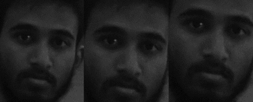 Fig. 1. Different face images resulting from the same class photo due to different bounding boxes. Left to right: Haar, DNN, and HOG.
The recognition algorithms were trained using eight images per student, 22 students, totaling 176 images. This training set was put together by using a photo of the student and then also rotating it through angles −15°,−10°,−5°,5°,10°, and 15°; the eighth image was obtained by adding Gaussian noise to the student image. Three different training sets were used corresponding to the relevant detection algorithms. Every recognition algorithm was trained with all three sets. This resulted in nine outputs for every face in every class. Detail regarding the experimental setup is given in Section IV.
Checking the prototype’s result against the actual attendees was done manually. A Microsoft Excel spreadsheet was used to record the data as follows: 1, if a person was correctly recognized, and 0, if not. These were then summarized to measure final performance.
D.RESEARCH PURPOSE
The purpose of this study was to compare the performance of different combinations of algorithms, taking different class sizes into account, in a field experiment using a prototype application and a smartphone camera.
E.ETHICAL CONSIDERATIONS
Ethical clearance was obtained, and all participants gave written permission for their photos to be used in publications related to the research. Participation was voluntary, and no one was negatively affected in any way.
F.TECHNICAL DETAIL
Visual Studio 2015 (using C++) was used for constructing the prototype, together with OpenCV and DLIB implementations of the algorithms using default parameters. The specifications of the computer that was used are as follows: Intel® Core™ i7-8550U CPU at 1.80 GHz 1.99 GHz with 8.00 GB RAM. The smartphone camera that was used is a Sony Xperia XA2 Ultra (Model H3213). The average time taken for detection per class photo: Haar (18 s), DNN (30 s), and HOG (1119 s). The HOG algorithm took much longer due to the upscaling of the image needed to detect the small faces.
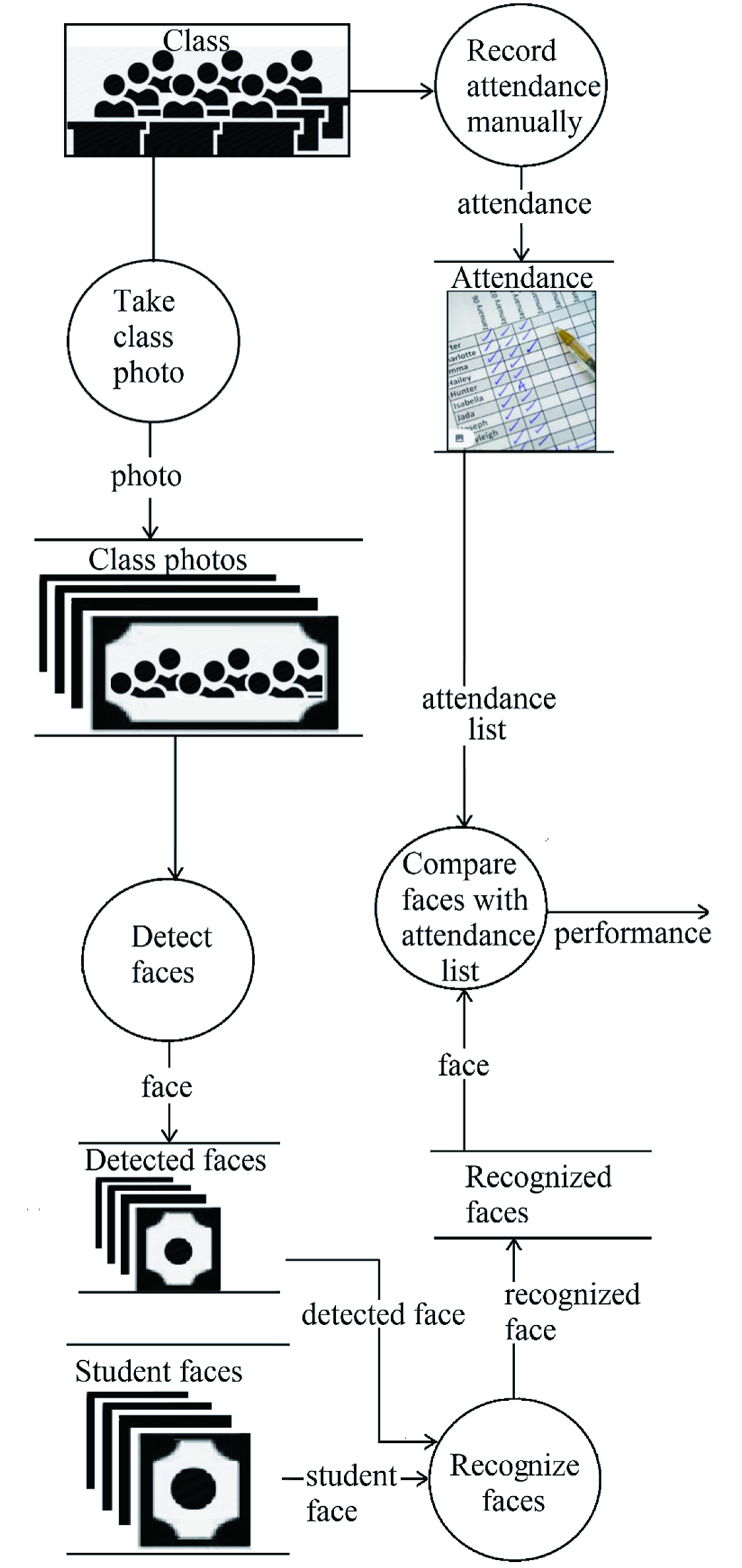
All the faces in a class photo were detected and saved as separate grayscale image files. Each face image was then queried against the training sets for the different recognition algorithms (matching with the detection algorithm used). A label was added to the image as the ID predicted by the algorithm. This label was then manually evaluated as being accurate or not. (It could not be evaluated programmatically because students were shuffled for every photo.) Fig. 2 illustrates the processes of the experiment.
G.CHALLENGES
According to the ethical clearance that was granted, no class time was to be used for this experiment. This resulted in a decision to use a public holiday. In turn, this presented challenges to get enough volunteers. Another major challenge that was experienced came from the smartphone that was used: even though no beauty feature was turned on, it does seem to “enhance” face photos automatically (it seems to enlarge the eyes). It also seems to “stretch” photos lengthwise. The ID photos of the students were taken in portrait format, whereas the class photos were taken in landscape format. This resulted in the lengthening of faces in the individual photos and the widening of faces in the class photos. Fig. 3 shows the difference between the ID photo that was taken and the face in the class photo (these photos were taken on the same day).
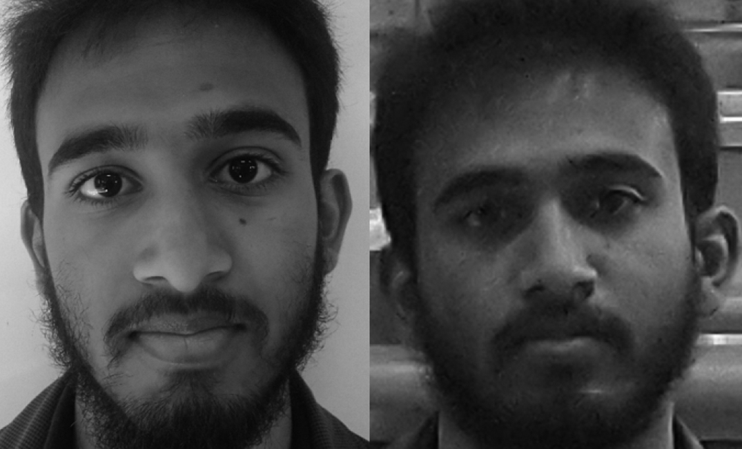 Fig. 3. ID photo taken versus photo cropped from class photo.
H.DATA ANALYSIS
The results were evaluated using some simple statistics, such as mean and standard deviation. Then a two-way analysis of variance (ANOVA) was used to determine if there are statistically significant differences between groups. Two more two-way ANOVAs were performed to determine if there are differences between the detection algorithms, and if there are differences between the recognition algorithms. Where significant differences were found, as indicated by the p-values, it was followed by Tukey tests to determine from where these differences originated.
IV.RESULTS
A.EXPERIMENTAL SETUP
Participants were asked to volunteer and to position themselves randomly for each “class” photo. The photos were taken from the front of the 10 m × 18 m class (the same class was used for all photos to ensure similar lighting conditions). Photos were taken at a resolution of 72 ppi × 72 ppi, resulting in 5984 pixel × 3376 pixel images. There were 30 photos taken: 15 of class size 10 and 15 of class size 22.
Table II shows an example of the raw data. Here follows some clarification regarding the data, e.g., student 01 in class DSC_0011:
- •correctly detected using Haar and consequently correctly recognized using fisherfaces and LBPH;
- •correctly detected using DNN and consequently correctly recognized using fisherfaces and LBPH; and
- •correctly detected using HOG, but not recognized using any of the recognition algorithms.
| Raw data as captured on Excel spreadsheet | ||||||
|---|---|---|---|---|---|---|
| Student | Class | Det | RE | RF | RL | |
| 01 | DSC_0011 | Haar | 1 | 0 | 1 | 1 |
| DNN | 1 | 0 | 1 | 1 | ||
| HOG | 1 | 0 | 0 | 0 | ||
| DSC_0012 | Haar | 1 | 0 | 1 | 1 | |
| DNN | 1 | 1 | 1 | 1 | ||
| HOG | 1 | 0 | 1 | 1 | ||
Det = correctly detected; RE = recognition with eigenfaces algorithm; RF = recognition with fisherfaces algorithm; and RL = recognition with LBPH.
The data were grouped together by class and detection algorithm, and then, for each detection algorithm, the performance of the recognition algorithms was calculated. Table III shows a sample of the summarized data per class.
| Summary of performance of algorithms | |||||
|---|---|---|---|---|---|
| Class size | 10 | Det | RE | RF | RL |
| DSC_0011 | Haar | 9 | 5 | 5 | 3 |
| DNN | 9 | 4 | 6 | 2 | |
| HOG | 10 | 4 | 4 | 2 | |
| DSC_0012 | Haar | 9 | 5 | 7 | 3 |
| DNN | 8 | 5 | 5 | 2 | |
| HOG | 8 | 1 | 4 | 1 | |
Det = correctly detected; RE = recognition with eigenfaces algorithm; RF = recognition with fisherfaces algorithm; and RL = recognition with LBPH.
In class DSC_0011, there were altogether:
- •nine students correctly detected with Haar of which five were correctly recognized using eigenfaces, five using fisherfaces, and three using LBPH;
- •nine students correctly detected with DNN of which four were correctly recognized using eigenfaces, six using fisherfaces, and two using LBPH; and
- •10 students correctly detected with HOG of which four were correctly recognized using eigenfaces, four using fisherfaces, and two using LBPH.
B.STATISTICAL ANALYSIS OF RESULTS
The graphs in Fig. 4 show how the different detection algorithms performed for the two different class sizes for each class.
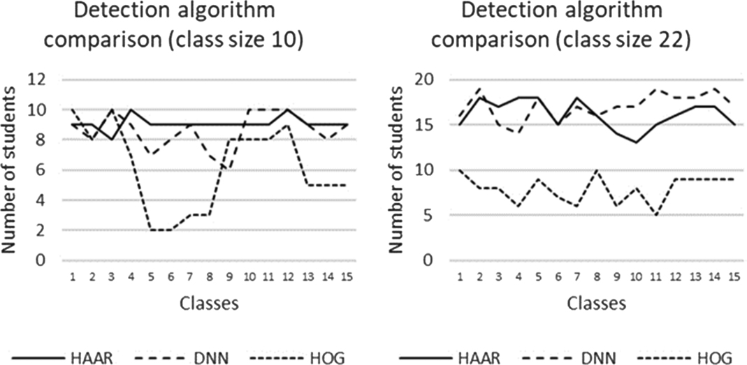 Fig. 4. Performance of detection algorithms.
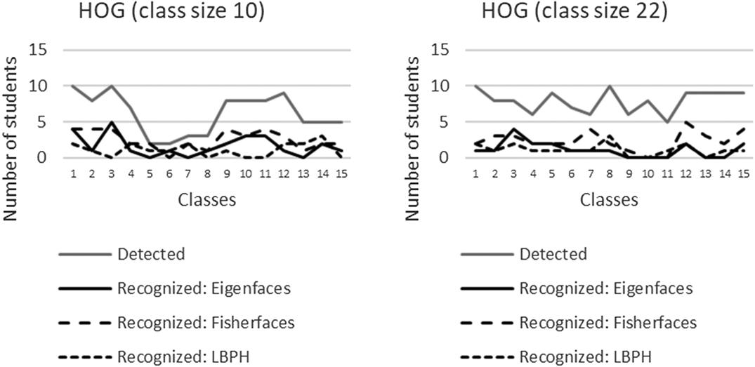
The results for the different detection algorithms together with the three recognition algorithms are summarized in Figs. 5–7.
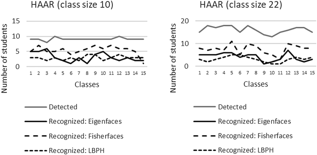 Fig. 5. Results—Haar algorithm (Viola–Jones).

C.MEANS
The means with the standard deviation for the number of correctly detected students are given in Fig. 8.
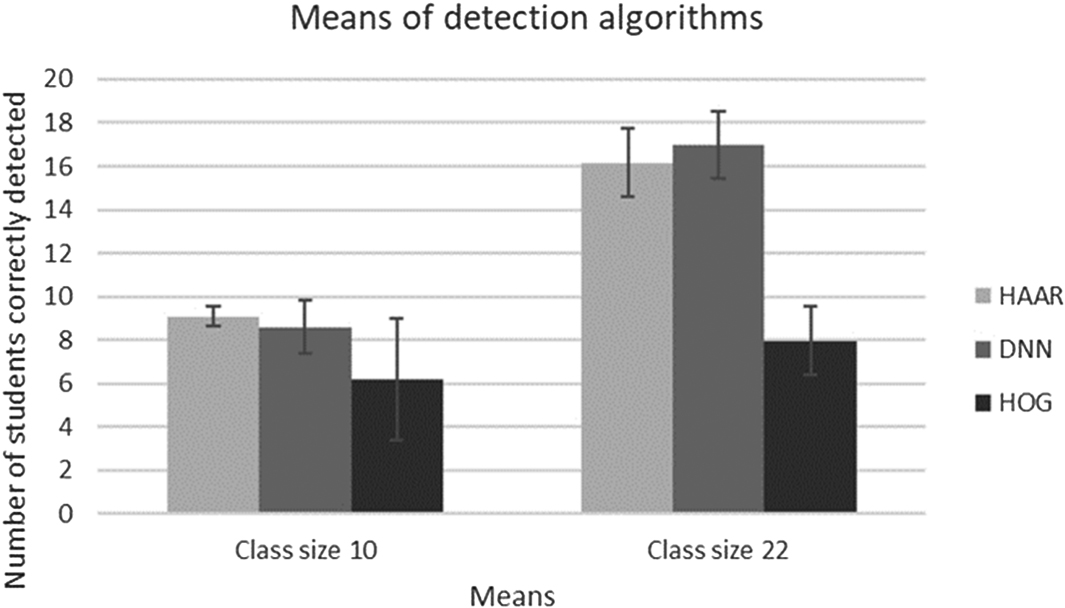 Fig. 8. Means of detection algorithms.
The graph in Fig. 9 shows the means for all nine of the algorithm combinations for the different class groups.
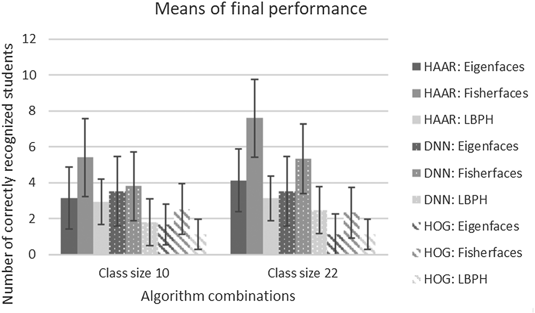 Fig. 9. Means for algorithm combinations.
For both class sizes (10 and 22), the Viola–Jones (Haar cascade) for detection together with fisherfaces for recognition performed the best.
D.ANOVA
A two-factor ANOVA with replication was done with the percentages of the results to find if there are statistically significant differences between the class sizes, as well as the different detection algorithms. An alpha level of 0.05 was used for all statistical tests. Table IV shows the results.
Table IV. Two-way ANOVA—Class Size Versus Detection
| ANOVA | ||||||
|---|---|---|---|---|---|---|
| Source of variation | SS | df | MS | F | p-value | F crit |
| Sample | 6760 | 1 | 6760 | 36.2701 | 4.4E-08 | 3.95457 |
| Columns | 21502.9 | 2 | 10751.4 | 57.6858 | 1.7E-16 | 3.10516 |
| Interaction | 1110.96 | 2 | 555.482 | 2.98038 | 0.05617 | 3.10516 |
| Within | 15655.9 | 84 | 186.379 | |||
| Total | 45029.7 | 89 | ||||
The two different class sizes are represented by the sample and the different detection algorithms by the columns in the table. For the samples (class sizes), there is a statistically significant difference [F(1,84) = 36.27, p < 0.001], meaning class size matters (no further tests were needed on the class sizes because there are only two different sizes). There are also statistically significant differences [F(2,84) = 57.69, p < 0.001] between the columns (detection algorithms). There are three columns. Further tests will provide more insight.
Further ANOVAs (two-factor with replication) were performed to determine if there are statistically significant differences between the class sizes and the recognition algorithms. Recognition is affected by detection, so they are not independent. For this reason, three different ANOVAs were done on the percentage values, different ones for each of the different detection algorithms. Tables V–VII show the results of the ANOVAs, where samples represent the class size, and the columns represent the different recognition algorithms. Each ANOVA represents a different detection algorithm.
Table V. ANOVA—Class Size Versus Recognition (Haar Detection)
| ANOVA | ||||||
|---|---|---|---|---|---|---|
| Source of variation | SS | df | MS | F | p-value | F crit |
| Sample | 5543.88 | 1 | 5543.88 | 47.0707 | 1.1E-09 | 3.95457 |
| Columns | 8853.85 | 2 | 4426.92 | 37.5871 | 2.2E-12 | 3.10516 |
| Interaction | 183.14 | 2 | 91.5702 | 0.77748 | 0.46284 | 3.10516 |
| Within | 9893.33 | 84 | 117.778 | |||
| Total | 24474.2 | 89 | ||||
Table VI. ANOVA—Class Size Versus Recognition (DNN Detection)
| ANOVA | ||||||
|---|---|---|---|---|---|---|
| Source of variation | SS | df | MS | F | p-value | F crit |
| Sample | 3963.72 | 1 | 3963.72 | 23.6587 | 5.3E-06 | 3.95457 |
| Columns | 4251.81 | 2 | 2125.9 | 12.6891 | 1.5E-05 | 3.10516 |
| Interaction | 587.163 | 2 | 293.581 | 1.75233 | 0.17965 | 3.10516 |
| Within | 14073.2 | 84 | 167.538 | |||
| Total | 22875.9 | 89 | ||||
Table VII. ANOVA—Class Size Versus Recognition (HOG Detection)
| ANOVA | ||||||
|---|---|---|---|---|---|---|
| Source of variation | SS | df | MS | F | p-value | F crit |
| Sample | 2628.33 | 1 | 2628.33 | 27.5553 | 1.1E-06 | 3.95457 |
| Columns | 1515.83 | 2 | 757.916 | 7.94596 | 0.00069 | 3.10516 |
| Interaction | 279.467 | 2 | 139.734 | 1.46496 | 0.23693 | 3.10516 |
| Within | 8012.23 | 84 | 95.3837 | |||
| Total | 12435.9 | 89 | ||||
There is a statistically significant difference [F(1,84) = 47.07, p < 0.001] for the samples (class sizes). There are also statistically significant differences [F(2,84) = 37.59, p < 0.001] between the columns (recognition algorithms). The ANOVA does not indicate from where these differences originate, so these results were further investigated using post hoc tests.
There are statistically significant differences [F(1,84) = 23.66, p < 0.001] for the samples (class sizes) and between the columns (recognition algorithms) [F(2,84) = 12.69, p < 0.001]. These results were further investigated.
The samples (class sizes) are statistically significantly different [F(1,84) = 27.56, p < 0.001]. The columns (detection algorithms) also differ [F(2,84) = 7.95, p < 0.001]. These results were further investigated.
E.TUKEY HSD
All the ANOVAs pointed to differences that needed to be further investigated. Tukey HSD showed the following statistically significant differences:
- •Between detection algorithms: Haar performed better than HOG (p < 0.001); DNN performed better than HOG (p < 0.001). Table VIII shows the results of the Tukey test for the detection algorithms.
- •Between recognition algorithms (within a specific detection algorithm):
- ∘Haar: Fisherfaces performed better than eigenfaces (p < 0.001); fisherfaces performed better than LBPH (p < 0.001). Table IX shows the Tukey results for the recognition algorithms.
- ∘DNN: Fisherfaces performed better than LBPH (p < 0.001); eigenfaces performed better than LBPH (p = 0.004). Table X shows the Tukey results between the recognition algorithms.
- ∘HOG: Fisherfaces performed better than eigenfaces (p = 0.017); fisherfaces performed better than LBPH (p < 0.001). Table XI shows the Tukey results for the recognition algorithms.
Table VIII. Tukey Results for the Detection Algorithms
| Tukey HSD; column effect | alpha | 0.050 | ||
|---|---|---|---|---|
| Group | Mean | Size | df | q-crit |
| DNN | 81.636 | 30.000 | ||
| Haar | 82.000 | 30.000 | ||
| HOG | 49.030 | 30.000 | ||
| 90.000 | 84.000 | 3.374 | ||
| Group 1 | Group 2 | Mean | Std err | q-stat | mean-crit | Lower | Upper | p-value | Cohen d |
|---|---|---|---|---|---|---|---|---|---|
| DNN | Haar | 0.364 | 2.493 | 0.146 | 8.410 | −8.046 | 8.773 | 0.994 | 0.027 |
| DNN | HOG | 32.606 | 2.493 | 13.082 | 8.410 | 24.196 | 41.016 | 3.77E-15 | 2.388 |
| Haar | HOG | 32.970 | 2.493 | 13.227 | 8.410 | 24.560 | 41.379 | 2.49E-14 | 2.415 |
Table IX. Tukey Results for the Recognition Algorithms Following Detection by Haar Algorithm
| Tukey HSD; column effect | alpha | 0.050 | ||
|---|---|---|---|---|
| Group | Mean | Size | df | q-crit |
| Eigenfaces% | 25.061 | 30.000 | ||
| Fisherfaces% | 44.273 | 30.000 | ||
| LBPH% | 21.788 | 30.000 | ||
| 90.000 | 84.000 | 3.374 | ||
| Q test | |||||||||
|---|---|---|---|---|---|---|---|---|---|
| Group 1 | Group 2 | Mean | std err | q-stat | Mean-crit | Lower | Upper | p-value | Cohen d |
| Eigenfaces% | Fisherfaces% | 19.212 | 1.981 | 9.696 | 6.685 | 12.527 | 25.897 | 3.33E-09 | 1.770 |
| Eigenfaces% | LBPH% | 3.273 | 1.981 | 1.652 | 6.685 | −3.412 | 9.958 | 0.476 | 0.302 |
| Fisherfaces% | LBPH% | 22.485 | 1.981 | 11.348 | 6.685 | 15.800 | 29.170 | 1.62E-11 | 2.072 |
Table X. Tukey Results for the Recognition Algorithms Following Detection by DNN Algorithm
| Tukey HSD; column effect | alpha | 0.050 | ||
|---|---|---|---|---|
| Group | Mean | Size | df | q-crit |
| Eigenfaces% | 25.697 | 30.000 | ||
| Fisherfaces% | 31.121 | 30.000 | ||
| LBPH% | 14.606 | 30.000 | ||
| 90.000 | 84.000 | 3.374 | ||
| Q test | |||||||||
|---|---|---|---|---|---|---|---|---|---|
| Group 1 | Group 2 | Mean | std err | q-stat | Mean-crit | Lower | Upper | p-value | Cohen d |
| Eigenfaces% | Fisherfaces% | 5.424 | 2.363 | 2.295 | 7.973 | −2.549 | 13.398 | 0.242 | 0.419 |
| Eigenfaces% | LBPH% | 11.091 | 2.363 | 4.693 | 7.973 | 3.118 | 19.064 | 0.004 | 0.857 |
| Fisherfaces% | LBPH% | 16.515 | 2.363 | 6.989 | 7.973 | 8.542 | 24.488 | 1.16E-05 | 1.276 |
Table XI. Tukey Results for the Recognition Algorithms Following Detection by HOG Algorithm
| alpha | 0.050 | |||
|---|---|---|---|---|
| Group | Mean | Size | df | q-crit |
| Eigenfaces % | 10.9091 | 30.000 | ||
| Fisherfaces % | 7.9708 | 30.000 | ||
| LBPH % | 242 | 30.000 | ||
| 90.000 | 84.000 | 3.374 | ||
| Group 1 | Group 2 | Mean | std err | q-stat | Mean-crit | Lower | Upper | p-value | Cohen d |
|---|---|---|---|---|---|---|---|---|---|
| Eigenfaces% | Fisherfaces% | 7.061 | 1.783 | 3.960 | 6.016 | 1.044 | 13.077 | 0.017 | 0.723 |
| Eigenfaces% | LBPH% | 2.667 | 1.783 | 1.496 | 6.016 | −3.350 | 8.683 | 0.543 | 0.273 |
| Fisherfaces% | LBPH% | 9.727 | 1.783 | 5.455 | 6.016 | 3.711 | 15.743 | 6.50E-04 | 0.996 |
V.DISCUSSION AND CONCLUSIONS
If the means are converted to percentages, the results are as follows:
- •Class size 10
- ∘Haar detected (M = 91%, SD = 5%)
- ▪Eigenfaces (M = 31%, SD = 16%)
- ▪Fisherfaces (M = 54%, SD = 15%)
- ▪LBPH (M = 29%, SD = 7%)
- ∘DNN (M = 86%, SD = 12%)
- ▪Eigenfaces (M = 35%, SD = 17%)
- ▪Fisherfaces (M = 38%, SD = 19%)
- ▪LBPH (M = 18%, SD = 13%)
- ∘HOG (M = 62%, SD = 28%)
- ▪Eigenfaces (M = 17%, SD = 15%)
- ▪Fisherfaces (M = 25%, SD = 13%)
- ▪LBPH (M = 11%, SD = 10%)
- ∘Haar detected (M = 91%, SD = 5%)
- •Class size 22
- ∘Haar (M = 72.7%, SD = 7.3%)
- ▪Eigenfaces (M = 18.6%, SD = 7.7%)
- ▪Fisherfaces (M = 34.5%, SD = 10%)
- ▪LBPH (M = 14.1%, SD = 5.5%)
- ∘DNN (M = 77.3%, SD = 7.3%)
- ▪Eigenfaces (M = 15.9%, SD = 8.6%)
- ▪Fisherfaces (M = 24.1%, SD = 8.6%)
- ▪LBPH (M = 11.4%, SD = 5.9%)
- ∘HOG (M = 35.9%, SD = 7.3%)
- ▪Eigenfaces (M = 5%, SD = 5%)
- ▪Fisherfaces (M = 10.5%, SD = 6.4%)
- ▪LBPH (M = 5%, SD = 3.6%)
- ∘Haar (M = 72.7%, SD = 7.3%)
A.BEST ALGORITHMS
1)DETECTION
The means of the detection functions are given in Fig. 8. Looking at the means of the detection only, it seems clear that the Haar function is the best algorithm for class size 10 and DNN for class size 22, but upon further analysis, the difference is not statistically significant. The HOG function did not perform well and is much slower than the Haar and DNN functions (18 and 29 s vs 1119 s, respectively, on average of a single class photo). At this point, it can be concluded that either the Haar or DNN function can be used (just purely focusing on detection alone).
The advantage of the DNN function over the Haar function is the fact that the Haar function returns many false positives, i.e., with current settings. Fine tuning might help, but at the expense of processing speed. The false positives were manually discarded, but it will be problematic in real-life implementation of the prototype. This experiment produced up to 20 false positives for class size 10 and up to 13 for class size 22. Just looking at class size 10, the Haar function is very stable (good straight-line graph—see Fig. 4, small standard deviation), but it is a problem when the subject wears glasses.
2)RECOGNITION
The recognition followed the detection process and as such is dependent on detection. The means, therefore, are calculated relative to a specific detection.
Again, just looking at the means, it seems that fisherfaces outperformed the eigenfaces and LBPH functions. Further analysis shows that fisherfaces performed statistically significantly better than the other functions, where Haar and HOG detection were used. At this point, it is worth mentioning that even though the DNN recognition function seemed to perform better on the larger class size, the combination of Haar detection and fisherfaces recognition performed better than any of the recognition algorithms following the DNN detection.
It needs to be mentioned that some resolution is lost in photos of students at the back of the class. Though they may be correctly detected, there may not be enough information left to correctly recognize the student. The same applies for partially occluded (obstructed) faces.
B.EFFECT OF CLASS SIZE
All the results are reported by differentiating between the different class sizes. The ANOVA showed that there is a statistically significant difference between the class sizes (see Fig. 4) for detection.
These means indicate that there is a significant decline in the detection for the larger class (and the ANOVA confirms the significance of this decline).
Looking at the outcome (percentages) for detection together with recognition again, there is a significant difference between the class groups (again the ANOVA confirms it). For the DNN detection combined with eigenfaces, the results declined with more than 50%.
C.ACCURACY AND OVERALL PERFORMANCE OF PROTOTYPE
The average performance of the different algorithms and combinations of algorithms have been discussed in the previous sections. It is worth mentioning that there were instances for class size 10, where all students were correctly detected (Haar: two cases; DNN: four cases; HOG: two cases). At best, seven of these students were correctly identified.
The best detection for class size 22 was 19, with at best six students being correctly identified. The maximum recognition was 7 out of 10 and 11 out of 22, respectively. These do not correspond with the best detections necessarily. This does not translate directly to an accuracy of 70% and 50% (for the recognition functions) because it depends on how many students were detected before the recognition commenced. For instance, seven students were correctly identified, but only nine were correctly detected, so that translates to a 77.8% performance for the recognition (if measured independently).
The distance of the students from the camera plays a role, since it affects the resolution of the face and, therefore, impacts on the recognition. The angle at which the photo of the student has been taken, can also impact on resolution. A possible solution to this might be to group students in the class into smaller groups and take a photo from relatively close by (also proposed by [18]). Fig. 10 shows an example of the loss of resolution in a typical class photo.
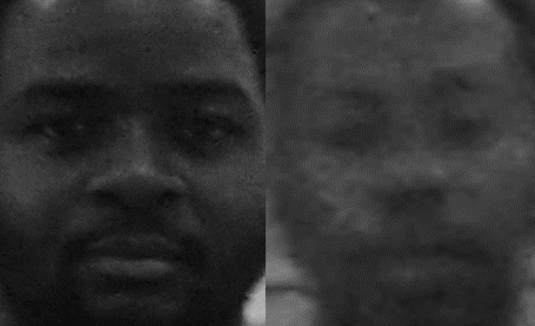 Fig. 10. Difference in resolution of student in the front of the class (left) versus student at the back of the class (right).
Ethnicity have been known to affect these algorithms with darker-skinned females the least likely to be correctly recognized, compared to their dark-skinned male and light-skinned male and female counterparts [45]. Individuals in the age group 18–30 are also at a disadvantage [46]. The rationale is that it is due to the training data being biased (for detection). For recognition, the fact that there is less contrast between features (such as eyebrows, hairlines, and lips) and skin color might play a role because the features are less prominent and consequently difficult to distinguish [47]. Unfortunately, the sample classes consisted of only darker-skinned individuals in the age group 18–30, which may have impacted on the accuracy of the algorithms.
Students wearing glasses, headdresses, or hats were often not detected and/or recognized.
D.COMPARISON WITH OTHER STUDIES/SYSTEMS
The studies by Samet and Tanriverdi [29] and Budi et al. [6] are the most closely related to this study because they also make use of smartphones. As mentioned before, the Samet and Tanriverdi [29] study had an accuracy of 84.81% at best for the case of more than three training images per student, if measured within what was detected. However, if this is measured against the actual attendance, it comes down to 60.9%.
This study’s results for class size 10 seem to be comparable (M = 54%, SD = 15%) and fairly acceptable considering the low cost of using an average smartphone camera and only single images.
Another interesting finding is the fact that in this study fisherfaces outperformed the other algorithms. The only other study that also had this finding was the one by Raghuwanshi and Swami [27].
VI.CONCLUSION
This study explored the possibility of using a smartphone camera in combination with face detection and recognition algorithms for recording class attendance. The performance of the prototype was not accurate enough to use as is, but with some adjustments, it can become an inexpensive solution to the attendance recording problem. These adjustments may be taking more photos of the class, breaking the class up into smaller groups, taking a video, fine tuning the algorithms or training them with more relevant data, obtaining more training images per student, or varying pose and angle. These adjustments will not add to the cost of the solution (or make it more cumbersome) and is worth exploring.