JAIT

I.INTRODUCTION

Real-world robotics applications, such as minimally invasive surgeries [1], home services [2], endoscope detection [3], on-orbit servicing [4], and field rescues [5], are different from the applications of conventional rigid-link manipulators, while in these cases the operation compliance, dexterity, and safety of the robot manipulators are more important than the operation accuracy. Driven by a large number of new application requirements, in the past three decades, developing the continuum manipulators have been given more attention in the robotics field.

By classifying the continuum manipulators according to their drive types, four classes of continuum manipulators, including continuously bending actuators [6], tendons [3], [7], [8], active cannulas [9], [10], and steerable needle [11], have been presented to date. Similar to rigid-link manipulators, the kinematics of the continuum manipulators are also related to three spaces, which are actuation space, configuration space, and task space. For many manipulator systems, the actuation space and the configuration space are not identical. Therefore, as presented by [11] and [12], in general, we should set up two level maps to describe the relationships of the three spaces and then to derive the kinematics model of the manipulators, which is commonly necessary to control the manipulators and realize the given operation task. Since the shape and the structure of a continuum manipulator are featured by an infinite degree of freedom (DOF) elastic member, parameterizing the configuration space of the continuum manipulators by a set of generalized coordinates is not as straightforward as that of rigid-link manipulators. For instance, Yang et al. [7] employed the finite element method to analyze the deformations of a flexible elephant trunk manipulator. Although the finite element method can provide good calculation accuracy, the high-dimensional system model is difficult to be utilized to control the manipulator in real time. Jones and Walker [13] presented a modified Denavit–Hartenberg (D–H) method to obtain the kinematics model of multisection continuum manipulators. However, the D–H method-based approaches are hard to be developed to modeling a variant curvature continuum manipulator. In [14], Hannan and Walker applied the Frenet–Serret (F–S) frames to get the forward kinematics of continuum manipulators. Under the assumption of constant-curvature, the F–S formulas-based model can be explicitly integrated, and the derived model agrees with that obtained by the other methods. However, F–S fame is undefined when the curvature of an elastic body equals zero.

Relatively, using exponential coordinates based on Lie group theory is a more general method for modeling the kinematics of continuum manipulators [11], [12]. Murray et al. [15] provided a thorough treatment of exponential coordinates on the basis of Lie group theory for modeling and analysis of different rigid-body robots. Webster et al. [11] developed this methodology to build the model and analyze the motions of flexible needles that have bevel tip. Closely related to the continuum manipulators, Wang et al. [16] used the same methodology to analyze the workspace of hyper-redundant manipulators. With the help of the concept of twists, which is the infinitesimal generator of the Euclidean group, and matrix exponential, which maps a twist into the corresponding screw motion, the inherent nonlinear characteristics of motions in the non-Euclidean configuration space of the continuum manipulators can be globally revealed more thoroughly, while without suffering from singularities due to the use of local coordinates, such as that arisen in the F–S frames and D–H method. In addition, the exponential coordinates-based methods provide a very geometric description of body’s motions, which greatly simplify the analysis of the differential kinematics of multibody mechanical systems. He [17] investigated the motion planning and saturation feedback control of endoscopic operations of continuum manipulators using screw theory.

Since the concentric tube robots [9], [10], [18], [19] and steerable needle robots [11], [12] are primarily developed for some specific applications of minimally invasive surgeries, the rather small bending stiffness makes it difficult for them to be applied to other fields. The continuously bending actuators-based continuum manipulators include two types. One type is actuated by flexible rods [6], [20], and the other type is actuated by pneumatic tubes [21], [22]. The former is commonly an elastic member with single or double segments and, thereby, shows certain poor manipulability in mechanisms. While the latter is generally limited by their rather heavy power supply systems and strong noises from the air compressor, so that they are not applicable to hospitals, schools, nursing homes, or other similar occasions. By comparison, the continuum manipulators actuated by tendons generally show more flexibility in mechanical systems design [1]–[4], [7], [12], larger range adjustable dynamic characteristics [2], and better adaptability in applications [2]–[4], [7], [23]–[25]. Considering these factors and our aim of developing a rehabilitation nursing robot, of which the main capabilities should at least include variable stiffness in compliant operation, large motion range, certain load capability, and dexterous manipulability. Therefore, we are interested in developing a continuum manipulator with multielastic segments and actuated by tendons.

The contributions of this paper are that, by applying the exponential coordinates based on the Lie group theory, a complete kinematics modeling process for general N-segment continuum manipulators actuated by tendons is presented. In [11] and [16], similar methods had also been applied to build the kinematics model of other type manipulators, which are different from the study object of this paper. On the basis of the inverse differential kinematics model, a novel motion planning approach is further presented, which is named as “dynamic coordination method” (DCM), for the continuum manipulators. The novel motion planning approach is featured by the follwing appealing properties: it is a programming method in global task space; it does not depend on any convex index function or convex assumption of the searching space; and it permits online dynamically adjust the characteristic points of concerns so that the calculation efficiency of the approach can be effectively improved for simple operation tasks.

This paper is organized as follows. In Section II, the forward kinematics of the continuum manipulators with piecewise constant curvatures are presented. In Section III, the differential kinematics is derived, and the complete Jacobian of the continuum manipulators is obtained. In Section IV, the motion planning of the continuum manipulators is discussed, and a novel approach named as DCM is presented. In Section V, the conclusions of this paper and some research directions in the future are presented.

II.KINEMATICS MODELING OF A CONTINUUM MANIPULATOR WITH PIECEWISE CONSTANT CURVATURES

Even though the tendon driven continuum manipulators show certain attractive features in design and applications, a drawback of this kind of robot is that the configuration space and the actuation space of the robot are not identical. From the viewpoint of kinematics modeling, this point brings some inconveniences, and two-level maps have been built, one from configuration space to task space and the other from actuation space to configuration space. And then the complete forward kinematics could be obtained.

A.THE KINEMATICS MODELING FROM CONFIGURATION SPACE TO TASK SPACE

Suppose that the continuum manipulator has segments, and every elastic segment deforms under a constant curvature along the backbone of the same segment. Note here the constant curvature means the curvature of single segment is instantaneously uniform, but it does not mean that the curvatures of all segments of the continuum manipulator are instantaneously uniform, and also does not mean the curvatures are invariant about time.

Fig. 1 shows a segment $o_{i - 1} - o_{i}$ , where the frame $\sum_{i - 1} (o_{i - 1} - x_{i - 1} y_{i - 1} z_{i - 1})$ is the base frame, which is fixed to the center of the cross section closing to the base, $\sum_{i} (o_{i} - x_{i} y_{i} z_{i})$ is the body frame, which is fixed to the center of the cross section far away from the base, the axes $z_{i - 1}$ and $z_{i}$ are tangential to the backbone arc, the dihedral angle $θ_{i - 1}$ is defined to be the angle between the top and bottom cross-sections, the torsion angle of the body with respect to the axis $z_{i - 1}$ is $φ_{i - 1}$ , the backbone’s arc length $ℓ_{i - 1}$ of all segments of the continuum manipulator can neither be compressed nor extended, and the frames $\sum_{i} (i = 1, 2, \dots, m)$ are established according to the left-hand rule. Thus, the elastic segments can be parameterized in configuration space as $Θ_{i - 1} = [\begin{matrix} κ_{i - 1} & φ_{i - 1} & ℓ_{i - 1} \end{matrix}]^{T}$ . By these assumptions, it is straightforward that the motion of the top cross section of the elastic segment $o_{i - 1} - o_{i}$ can be decomposed into a rotation about the axis $z_{i - 1}$ and an in-plane curl deformation. Associated with the two decomposed motions, the corresponding twist coordinates can be written as

ξ_{r o t} = [\begin{matrix} υ_{r o t} \\ ω_{r o t} \end{matrix}] = [\begin{matrix} 0 & 0 & 0 & 0 & 0 & 1 \end{matrix}]^{T}

(1)

and

ξ_{i n p} = [\begin{matrix} υ_{i n p} \\ ω_{i n p} \end{matrix}] = [\begin{matrix} 0 & 0 & 1 & 0 & κ_{i - 1} & 0 \end{matrix}]^{T},

(2)

where

υ \in ℜ^{3}

and

ω \in ℜ^{3}

are linear and angular differential motions, respectively, and

κ_{i - 1}

is the curvature of the elastic segment

o_{i - 1} - o_{i}

. The twists of the twist coordinates (1) and (2) can be written as

{\hat{ξ}}_{r o t} = [\begin{matrix} {\hat{ω}}_{r o t} & υ_{r o t} \\ 0 & 0 \end{matrix}] = [\begin{matrix} 0 & - 1 & 0 & 0 \\ 1 & 0 & 0 & 0 \\ 0 & 0 & 0 & 0 \\ 0 & 0 & 0 & 0 \end{matrix}]

(3)

and

{\hat{ξ}}_{i n p} = [\begin{matrix} {\hat{ω}}_{i n p} & υ_{i n p} \\ 0 & 0 \end{matrix}] = [\begin{matrix} 0 & 0 & κ_{i - 1} & 0 \\ 0 & 0 & 0 & 0 \\ - κ_{i - 1} & 0 & 0 & 1 \\ 0 & 0 & 0 & 0 \end{matrix}],

(4)

respectively, where the symbol “

\land

” indicates the wedge operator [15], which maps a vector from

ℜ^{3}

to the Lie algebra

s o (3)

of the Lie group

S O (3)

, or maps a vector from

ℜ^{6}

to the Lie algebra

s e (3)

of the Lie group

S E (3)

. By applying the product of exponentials formula [12], [15], the transformation from the tip frame

\sum_{i}

to the base frame

\sum_{i - 1}

is given by

T_{i}^{i - 1} = \exp ({\hat{ξ}}_{r o t} φ_{i - 1}) \exp ({\hat{ξ}}_{i n p} ℓ_{i - 1}),

(5)

where the matrix exponential of the net rotation in (5) is given by

\exp ({\hat{ξ}}_{r o t} φ_{i - 1}) = [\begin{matrix} e^{({\hat{ω}}_{r o t} φ_{i - 1})} & 0 \\ 0 & 1 \end{matrix}],

(6)

while the matrix exponential of the in-plane motion in (5) is given by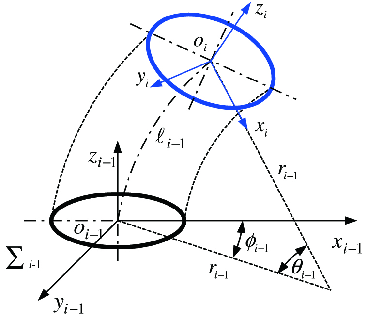

\exp ({\hat{ξ}}_{i n p} ℓ_{i - 1}) = [\begin{matrix} e^{({\hat{ω}}_{i n p} ℓ_{i - 1})} & \frac{(I - e^{({\hat{ω}}_{i n p} ℓ_{i - 1})}) {\hat{ω}}_{i n p} υ_{i n p} + ω_{i n p} ω_{i n p}^{T} υ_{i n p} ℓ_{i - 1}}{{‖ ω_{i n p} ‖}^{2}} \\ 0 & 1 \end{matrix}] .

(7)

Fig. 1. Parameters of a segment of a continuum manipulator in configuration space.

Then, substituting (6) and (7) into (5), the transformation (5) can be written as

T_{i}^{i - 1} = [\begin{matrix} R_{i}^{i - 1} & P_{i}^{i - 1} \\ 0 & 1 \end{matrix}],

(8)

where

R_{i}^{i - 1} = e^{({\hat{ω}}_{r o t} φ_{i - 1})} e^{({\hat{ω}}_{i n p} ℓ_{i - 1})}

(9)

and

P_{i}^{i - 1} = e^{({\hat{ω}}_{r o t} φ_{i - 1})} \times [(I - e^{({\hat{ω}}_{i n p} ℓ_{i - 1})}) \frac{{\hat{ω}}_{i n p}}{{‖ ω_{i n p} ‖}^{2}} υ_{i n p} + \frac{1}{{‖ ω_{i n p} ‖}^{2}} ω_{i n p} ω_{i n p}^{T} υ_{i n p} ℓ_{i - 1}] .

(10)

Note that $‖ ω_{r o t} ‖ = 1$ , thus by using the Rodrigues’ formula [15], the special orthogonal group $e^{({\hat{ω}}_{r o t} φ_{i - 1})} \in S O (3)$ can be calculated by

e^{({\hat{ω}}_{r o t} φ_{i - 1})} = I + {\hat{ω}}_{r o t} \sin φ_{i - 1} + {\hat{ω}}_{r o t}^{2} (1 - \cos φ_{i - 1}) = [\begin{matrix} \cos φ_{i - 1} & - \sin φ_{i - 1} & 0 \\ \sin φ_{i - 1} & \cos φ_{i - 1} & 0 \\ 0 & 0 & 1 \end{matrix}]

(11)

and owing to

‖ ω_{i n p} ‖ = κ_{i - 1} \neq 1, κ_{i - 1} = 1 / r_{i - 1}, θ_{i - 1} = κ_{i - 1} ℓ_{i - 1}, and d ℓ_{i - 1} / d t = 0 .

(12)

The special Euclidean group

e^{({\hat{ω}}_{i n p} ℓ_{i - 1})} \in S E (3)

is calculated by

e^{({\hat{ω}}_{i n p} ℓ_{i - 1})} = I + \frac{{\hat{ω}}_{i n p}}{‖ ω_{i n p} ‖} \sin (‖ ω_{i n p} ‖ ℓ_{i - 1}) + \frac{{\hat{ω}}_{i n p}^{2}}{{‖ ω_{i n p} ‖}^{2}} [1 - \cos (‖ ω_{i n p} ‖ ℓ_{i - 1})] = [\begin{matrix} \cos θ_{i - 1} & 0 & \sin θ_{i - 1} \\ 0 & 1 & 0 \\ - \sin θ_{i - 1} & 0 & \cos θ_{i - 1} \end{matrix}] .

(13)

Thus by using (11) and (13), the rotation group (9) can be calculated as

R_{i}^{i - 1} = [\begin{matrix} \cos φ_{i - 1} \cos θ_{i - 1} & - \sin φ_{i - 1} & \cos φ_{i - 1} \sin θ_{i - 1} \\ \sin φ_{i - 1} \cos θ_{i - 1} & \cos φ_{i - 1} & \sin φ_{i - 1} \sin θ_{i - 1} \\ - \sin θ_{i - 1} & 0 & \cos θ_{i - 1} \end{matrix}] .

(14)

To get the explicit expression of the position vector $P_{i}^{i - 1}$ in (10), it can be shown that the second term of the right-hand side of (10) satisfies

e^{({\hat{ω}}_{r o t} φ_{i - 1})} ω_{i n p} ω_{i n p}^{T} υ_{i n p} ℓ_{i - 1} = 0

due to

ω_{i n p}^{T} υ_{i n p} = [\begin{matrix} 0 & κ_{i-1} & 0 \end{matrix}] [\begin{matrix} 0 & 0 & 1 \end{matrix}]^{T} = 0

, thus from (10) we have

P_{i}^{i - 1} = e^{({\hat{ω}}_{r o t} φ_{i - 1})} (I - e^{({\hat{ω}}_{i n p} ℓ_{i - 1})}) \frac{{\hat{ω}}_{i n p}}{{‖ ω_{i n p} ‖}^{2}} υ_{i n p} = \frac{1}{κ_{i - 1}} [\begin{matrix} \cos φ_{i - 1} (1 - \cos θ_{i - 1}) \\ \sin φ_{i - 1} (1 - \cos θ_{i - 1}) \\ \sin θ_{i - 1} \end{matrix}] .

(15)

Considering (14) and (15), the homogeneous transformation matrix (8) of a segment from the configuration space to task space can be obtained. For overall the manipulator, the corresponding homogeneous transformation matrix can be written as

T_{m}^{0} = T_{1}^{0} T_{2}^{1} T_{3}^{2} \dots \dots T_{m}^{m - 1} = [\begin{matrix} R_{m}^{0} & P_{m}^{0} \\ 0 & 1 \end{matrix}] .

(16)

It is worth mentioning that the homogeneous transformation matrix $T_{i}^{i - 1} \in ℜ^{4 \times 4}$ is also a Euclidean group $T_{i}^{i - 1} \in S E (3)$ . Equations (8) and (16) are just the homogeneous representations of the Euclidean groups $T_{i}^{i - 1} \in S E (3)$ and $T_{m}^{0} \in S E (3)$ , respectively. From the viewpoint of Lie groups and with the help of exponential coordinates of twists, the inverse differential kinematics of the continuum manipulators can be analyzed more handily than by directly using the homogeneous representations (16), as will be shown in section III.

B.THE KINEMATICS MODELING FROM ACTUATION SPACE TO CONFIGURATION SPACE

In this paper, the segments $o_{i - 1} - o_{i} (i = 1, 2, 3, \dots, m)$ of the continuum manipulators are assumed to be actuated by three tendons, which are uniformly distributed with regard to the cross sections of all segments, then in the actuation space, the elastic segments can be parameterized as $q_{i - 1} = [\begin{matrix} l_{i - 1, 1} & l_{i - 1, 2} & l_{i - 1, 3} \end{matrix}]^{T}$ . In Fig. 2, let $φ_{i - 1, j} (j = 1, 2, 3)$ be the angles between the radius at the passing through points of the tendons in the base cross section and the plane $A - o_{i - 1} - o_{i}$ , then it is not difficult to show that

r_{i - 1, j} = r_{i - 1} - R_{i - 1} \cos φ_{i - 1, j} for j = 1, 2, 3 .

(17)

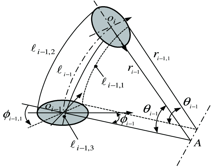Fig. 2. The relationship between the actuation space and the configuration space.

Considering the passing through points of the tendons which are distributed uniformly around the base cross section, without loss of generality, we have

φ_{i - 1, 1} = \frac{π}{2} + φ_{i - 1}, φ_{i - 1, 2} = \frac{7 π}{6} + φ_{i - 1}, and φ_{i - 1, 3} = \frac{11 π}{6} + φ_{i - 1} .

(18)

Owing to $r_{i - 1, j} θ_{i - 1} = ℓ_{i - 1, j}$ and $r_{i - 1} θ_{i - 1} = ℓ_{i - 1}$ under the assumption of piecewise constant curvatures, from (17) it follows that

ℓ_{i - 1, j} = ℓ_{i - 1} - R_{i - 1} θ_{i - 1} \cos φ_{i - 1, j} for j = 1, 2, 3 .

(19)

From (18) it is straightforward that $\sum_{j = 1}^{3} \cos φ_{i - 1, j} = 0$ , thereby, from (19) we have

ℓ_{i - 1} = \frac{1}{3} \sum_{j = 1}^{3} ℓ_{i - 1, j} .

(20)

By the first two equations of (19) (for $j = 1, 2$ ), it can be obtained that

R_{i - 1} θ_{i - 1} = \frac{ℓ_{i - 1, 2} - ℓ_{i - 1, 1}}{\cos φ_{i - 1, 1} - \cos φ_{i - 1, 2}} = \frac{ℓ_{i - 1, 2} - ℓ_{i - 1, 1}}{- \frac{3}{2} \sin φ_{i - 1} + \frac{\sqrt{3}}{2} \cos φ_{i - 1}},

(21)

and by the first and the third equations of (19) (for

j = 1, 3

), it also can be found that

R_{i - 1} θ_{i - 1} = \frac{ℓ_{i - 1, 3} - ℓ_{i - 1, 1}}{\cos φ_{i - 1, 1} - \cos φ_{i - 1, 3}} = \frac{ℓ_{i - 1, 3} - ℓ_{i - 1, 1}}{- \frac{3}{2} \sin φ_{i - 1} - \frac{\sqrt{3}}{2} \cos φ_{i}} .

(22)

From (21) and (22), we have

\tan φ_{i - 1} = \frac{2 ℓ_{i - 1, 1} - ℓ_{i - 1, 2} - ℓ_{i - 1, 3}}{\sqrt{3} (ℓ_{i - 1, 2} - ℓ_{i - 1, 3})} .

(23)

As shown in Fig. 2 and given by Fig. 3, if tendon’s planes parallel to plane $A - o_{i - 1} - o_{i}$ of the elastic segments are drawn, the following equations can be obtained:

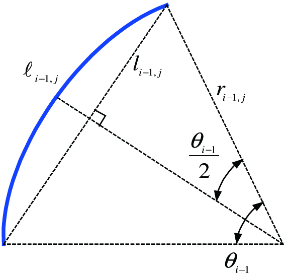ℓ_{i - 1, j} = r_{i - 1, j} θ_{i - 1} = \frac{l_{i - 1, j}}{2 \sin \frac{θ_{i - 1}}{2}} θ_{i - 1} = (\frac{θ_{i - 1}}{2 \sin \frac{θ_{i - 1}}{2}}) l_{i - 1, j}

(24)

Fig. 3. The geometric relationship of the tendon’s planes that are paralleling to the flexure plane of the elastic segments.

Define the coefficient $λ_{i - 1} = \frac{θ_{i - 1}}{2 \sin (θ_{i - 1} / 2)}$ , from (24) we have

ℓ_{i - 1, j} = λ_{i - 1} l_{i - 1, j} .

(25)

Substituting (25) into (23), it can be obtained the arc parameter $φ_{i - 1}$ that is a function of the length of tendons, so from (23) it follows that

φ_{i - 1} (q_{i - 1}) = \tan^{- 1} (\frac{2 l_{i - 1, 1} - l_{i - 1, 2} - l_{i - 1, 3}}{\sqrt{3} (l_{i - 1, 2} - l_{i - 1, 3})}) for i = 1, 2, 3, \dots, m .

(26)

To obtain the curvature represented by the parameters of actuation space, from (19) it can be shown that

θ_{i - 1} = \frac{ℓ_{i - 1} - ℓ_{i - 1, j}}{R_{i - 1} \cos φ_{i - 1, j}} .

(27)

Considering the fact $θ_{i - 1} = κ_{i - 1} ℓ_{i - 1}$ , so (27) for $j = 1$ can be rewritten as

κ_{i - 1} = \frac{ℓ_{i - 1} - ℓ_{i - 1, 1}}{R_{i - 1} ℓ_{i - 1} \cos φ_{i - 1, 1}} .

(28)

In (18), we note that $φ_{i - 1, 1} = \frac{π}{2} + φ_{i - 1}$ , thereby, $\cos φ_{i - 1, 1} = - \frac{1}{2} \sin φ_{i - 1}$ , and then (28) can be rewritten as

κ_{i - 1} = \frac{2 (ℓ_{i - 1, 1} - ℓ_{i - 1})}{R_{i - 1} ℓ_{i - 1} \sin φ_{i - 1}} .

(29)

By applying (20) and (25), and considering the following fact:

\sin φ_{i - 1} = \sin (\tan^{- 1} (\frac{y}{x})) = \frac{y}{\sqrt{x^{2} + y^{2}}}

(30)

The curvature (28) represented by the length of the tendons can be obtained as

κ_{i - 1} (q_{i - 1}) = \frac{2 \sqrt{l_{i - 1, 1}^{2} + l_{i - 1, 2}^{2} + l_{i - 1, 3}^{2} - l_{i - 1, 1} l_{i - 1, 2} - l_{i - 1, 1} l_{i - 1, 3} - l_{i - 1, 2} l_{i - 1, 3}}}{R_{i - 1} (l_{i - 1, 1} + l_{i - 1, 2} + l_{i - 13})}

(31)

for

i = 1, 2, 3, \dots, m

. Then, the forward kinematics from actuation space to configuration space of the continuum manipulators are given by (26) and (31).

This paper supposes that the continuum manipulator with a flexible backbone that is neither compressible nor extendable along the axial direction, and the arc length $ℓ_{i - 1}$ of a segment’s backbone cannot be adjusted by the three independent actuation inputs $q_{i - 1} \in ℜ^{3}$ . Therefore, every segment of the continuum manipulator is an over-actuated system. The major advantages of adopting an over-actuation scheme are that the stiffness of the “soft” manipulators in configuration space can be dexterously adjusted by controlling the non-zero internal forces of the elastic segments, and the structure clearances of the manipulators and the hysteresis effects caused by friction can be effectively reduced or even eliminated. As shown in [6] about a multibackbone continuum robot, these capabilities provided by over-actuation scheme for the continuum manipulators are appealing in practice.

III.DIFFERENTIAL KINEMATICS OF THE CONTINUUM MANIPULATORS

For a full actuation manipulator system, regardless of whether the mechanism of the manipulator is open linkage or closed linkage, searching for the inverse kinematics at coordinate variables level is commonly useful [15], since the dimension of the configuration space and that of the actuation space are identical, except a few of singularity points that possibly exist in either configuration space or actuation space. Thus, except these singularity points there always exists global inverse maps of the forward kinematics, such that under certain conditions the inverse kinematics is solvable, and the inverse solution is unique at most of configurations of the manipulators in their accessible configuration space. However, for an over-actuation mechanism, since the dimension of the actuation space is greater than that of the configuration space, there does not exist globally invertible maps between the actuation space and configuration space. Therefore, with regard to either a redundant DOFs manipulator or an over-actuated manipulator, the inverse kinematics need to be locally solved by the aids of the differential kinematics. Neppali et al. [26] presented an approach to solve the closed-form inverse kinematics of continuum manipulators. It is worth noting that the inverse kinematics from the task space to configuration space had just been considered in [26], and the approach is only valid for three segment continuum manipulators, since under this condition the inverse kinematics is unique, except for a few of singularity points.

Now let’s consider the Euclidean groups $T_{m}^{0} \in S E (3)$ that are given by (16),

T_{m}^{0} = [\begin{matrix} R_{m}^{0} & P_{m}^{0} \\ 0 & 1 \end{matrix}]

(32)

and

{\dot{T}}_{m}^{0} {(T_{m}^{0})}^{- 1} = [\begin{matrix} {\dot{R}}_{m}^{0} & {\dot{P}}_{m}^{0} \\ 0 & 0 \end{matrix}] [\begin{matrix} {(R_{m}^{0})}^{T} & - {(R_{m}^{0})}^{T} P_{m}^{0} \\ 0 & 1 \end{matrix}] = [\begin{matrix} {\dot{R}}_{m}^{0} {(R_{m}^{0})}^{T} & - {\dot{R}}_{m}^{0} {(R_{m}^{0})}^{T} P_{m}^{0} + {\dot{P}}_{m}^{0} \\ 0 & 0 \end{matrix}] .

(33)

It is interesting that the right-hand side of (33) shows a form of a twist, and the twist happens to be the velocity twist ${\hat{V}}_{m}^{0} \in s e (3)$ associated with the Euclidean groups $T_{m}^{0} \in S E (3)$ . From (33), the velocity vector of the tip frame $\sum_{m}$ represented in the inertial frame $\sum_{0}$ can be written as a form in twist coordinates, that is given by

V_{m}^{0} = [\begin{matrix} υ_{m}^{0} \\ ω_{m}^{0} \end{matrix}] = [\begin{matrix} - {\dot{R}}_{m}^{0} {(R_{m}^{0})}^{T} P_{m}^{0} + {\dot{P}}_{m}^{0} \\ {({\dot{R}}_{m}^{0} {(R_{m}^{0})}^{T})}^{\lor} \end{matrix}],

(34)

where the symbol “

\lor

” indicate the “vee” operator, which is the inverse operator of the “wedge” operator “

\land

.” In principle, the Jacobian of the manipulators can be obtained from (34); however, this will be a rather involved task for a multisegments continuum manipulator. Another approach to obtain the Jacobian of the manipulators is to use the definition of Jacobian. From (33) and (34), we have

{\hat{V}}_{m}^{0} = {\dot{T}}_{m}^{0} {(T_{m}^{0})}^{- 1} = \sum_{i = 1}^{m} (\frac{\partial T_{i}^{0}}{\partial Θ_{i - 1}} {(T_{m}^{0})}^{- 1}) {\dot{Θ}}_{i - 1} .

(35)

In twist coordinates, (35) can be written as

V_{m}^{0} = J_{m}^{0} {\dot{Θ}}_{i - 1},

(36)

where the Jacobian is given by

J_{m}^{0} = [\begin{matrix} (\frac{\partial T_{i}^{0}}{\partial Θ_{0}} {(T_{m}^{0})}^{- 1})^{\lor} & \dots & (\frac{\partial T_{i}^{0}}{\partial Θ_{m - 1}} {(T_{m}^{0})}^{- 1})^{\lor} \end{matrix}],

(37)

and the elements of (37) can be calculated by

\frac{\partial T_{i}^{0}}{\partial Θ_{i - 1}} {(T_{m}^{0})}^{- 1} = T_{i - 1}^{0} \frac{\partial T_{i}^{i - 1}}{\partial Θ_{i - 1}} T_{m}^{i} {(T_{m}^{0})}^{- 1} = T_{i - 1}^{0} \frac{\partial T_{i}^{i - 1}}{\partial Θ_{i - 1}} T_{m}^{i} {(T_{m}^{i})}^{- 1} {(T_{i - 1}^{0})}^{- 1} = T_{i - 1}^{0} \frac{\partial T_{i}^{i - 1}}{\partial Θ_{i - 1}} {(T_{i - 1}^{0})}^{- 1} .

(38)

By converting to twist coordinates, it follows that

(\frac{\partial T_{i}^{0}}{\partial Θ_{i - 1}} {(T_{m}^{0})}^{- 1})^{\lor} = {Ad}_{T_{i - 1}^{0}} {(\frac{\partial T_{i}^{i - 1}}{\partial Θ_{i - 1}})}^{\lor},

(39)

where

{Ad}_{T_{i - 1}^{0}} \in ℜ^{6 \times 6}

is defined to be the adjoint transformation of the group

T_{i - 1}^{0} \in ℜ^{4 \times 4}

, and that is given by

{Ad}_{T_{i - 1}^{0}} = [\begin{matrix} R_{i - 1}^{0} & {\hat{P}}_{i - 1}^{0} R_{i - 1}^{0} \\ 0 & R_{i - 1}^{0} \end{matrix}],

(40)

and

{(\frac{\partial T_{i}^{i - 1}}{\partial Θ_{i - 1}})}^{\lor}

is the local Jacobian

{[J_{c}]}_{i}^{i - 1}

of the segment

o_{i - 1} - o_{i}

in the frame

\sum_{i - 1}

, where the subscript “c” of

{[J_{c}]}_{i}^{i - 1}

indicates the Jacobian maps the velocity

{\dot{Θ}}_{i - 1}

from configuration space to task space. It is obvious that calculating the Jacobian (37) can be effectively simplified with the help of adjoint transformation

{Ad}_{T_{i - 1}^{0}}

. To calculate the Jacobian

{[J_{c}]}_{i}^{i - 1}

, the velocity

V_{i}^{i - 1}

of the segment

o_{i - 1} - o_{i}

is analyzed in the frame

\sum_{i - 1}

. From (33) and (34), it is straightforward that

{\hat{V}}_{i}^{i - 1} = {\dot{T}}_{i}^{i - 1} {(T_{i}^{i - 1})}^{- 1} = [\begin{matrix} {\dot{R}}_{i}^{i - 1} {(R_{i}^{i - 1})}^{T} & - {\dot{R}}_{i}^{i - 1} {(R_{i}^{i - 1})}^{T} P_{i}^{i - 1} + {\dot{P}}_{i}^{i - 1} \\ 0 & 1 \end{matrix}],

(41)

where

{\dot{R}}_{i}^{i - 1} = \frac{d}{d t} [e^{({\hat{ω}}_{r o t} φ_{i - 1})} e^{({\hat{ω}}_{i n p} ℓ_{i - 1})}] = {\hat{ω}}_{r o t} {\dot{φ}}_{i - 1} e^{({\hat{ω}}_{r o t} φ_{i - 1})} e^{({\hat{ω}}_{i n p} ℓ_{i - 1})} + ℓ_{i - 1} {\dot{κ}}_{i - 1} e^{({\hat{ω}}_{r o t} φ_{i - 1})} \frac{\partial {\hat{ω}}_{i n p}}{\partial κ_{i - 1}} e^{({\hat{ω}}_{i n p} ℓ_{i - 1})} .

(42)

If we define $e_{j} \in ℜ^{3}$ for $j = 1, 2, 3$ to be the unit vectors of the frame $\sum_{i - 1}$ , then we have

{\hat{ω}}_{r o t} = {\hat{e}}_{3} and {\hat{ω}}_{i n p} = κ_{i - 1} {\hat{e}}_{2},

(43)

and thereby, the twists have forms

{\hat{ξ}}_{i n p} = [\begin{matrix} κ_{i - 1} {\hat{e}}_{2} & e_{3} \\ 0 & 1 \end{matrix}] and {\hat{ξ}}_{r o t} = [\begin{matrix} {\hat{e}}_{3} & 0 \\ 0 & 1 \end{matrix}] .

(44)

Thus the element ${\dot{R}}_{i}^{i - 1} {(R_{i}^{i - 1})}^{T}$ of (41) can be given as

{\hat{ω}}_{i}^{i - 1} = {\dot{R}}_{i}^{i - 1} {(R_{i}^{i - 1})}^{T} = {\hat{e}}_{3} {\dot{φ}}_{i - 1} + {\hat{e}}_{2} ℓ_{i - 1} \cos φ_{i - 1} {\dot{κ}}_{i - 1} - {\hat{e}}_{1} ℓ_{i - 1} \sin φ_{i - 1} {\dot{κ}}_{i - 1} .

(45)

From (10), the term $- {\dot{R}}_{i}^{i - 1} {(R_{i}^{i - 1})}^{T} P_{i}^{i - 1}$ in (41) can be calculated by

- {\dot{R}}_{i}^{i - 1} {(R_{i}^{i - 1})}^{T} P_{i}^{i - 1} = - {\hat{ω}}_{i}^{i - 1} P_{i}^{i - 1} = - ({\hat{e}}_{3} {\dot{φ}}_{i - 1} + ℓ_{i - 1} {\dot{κ}}_{i - 1} {Ad}_{e^{({\hat{e}}_{3} φ_{i - 1})}} {\hat{e}}_{2}) e^{({\hat{ω}}_{r o t} φ_{i - 1})} (I - e^{({\hat{ω}}_{i n p} ℓ_{i - 1})}) \frac{1}{κ_{i - 1}} e_{1} = - {\hat{e}}_{3} e^{({\hat{ω}}_{r o t} φ_{i - 1})} (I - e^{({\hat{ω}}_{i n p} ℓ_{i - 1})}) \frac{1}{κ_{i - 1}} e_{1} {\dot{φ}}_{i - 1} - ℓ_{i - 1} {Ad}_{e^{({\hat{e}}_{3} φ_{i - 1})}} {\hat{e}}_{2} e^{({\hat{ω}}_{r o t} φ_{i - 1})} (I - e^{({\hat{ω}}_{i n p} ℓ_{i - 1})}) \frac{1}{κ_{i - 1}} e_{1} {\dot{κ}}_{i - 1},

(46)

and the velocity

{\dot{P}}_{i}^{i - 1}

in (41) can be calculated as

{\dot{P}}_{i}^{i - 1} = \frac{d}{d t} [e^{({\hat{ω}}_{r o t} φ_{i - 1})} (I - e^{({\hat{ω}}_{i n p} ℓ_{i - 1})}) \frac{{\hat{e}}_{2}}{κ_{i - 1}} e_{3}] = {\hat{e}}_{3} e^{({\hat{ω}}_{r o t} φ_{i - 1})} (I - e^{({\hat{ω}}_{i n p} ℓ_{i - 1})}) \frac{1}{κ_{i - 1}} e_{1} {\dot{φ}}_{i - 1} - ℓ_{i - 1} e^{({\hat{ω}}_{r o t} φ_{i - 1})} {\hat{e}}_{2} e^{({\hat{ω}}_{i n p} ℓ_{i - 1})} \frac{1}{κ_{i - 1}} e_{1} {\dot{κ}}_{i - 1} - e^{({\hat{ω}}_{r o t} φ_{i - 1})} (I - e^{({\hat{ω}}_{i n p} ℓ_{i - 1})}) \frac{1}{κ_{i - 1}^{2}} e_{1} {\dot{κ}}_{i - 1} .

(47)

Substituting (45), (46), and (47) into (41), it follows that

V_{i}^{i - 1} = {[J_{c}]}_{i}^{i - 1} [\begin{matrix} {\dot{κ}}_{i - 1} \\ {\dot{φ}}_{i - 1} \end{matrix}],

(48)

where

{[J_{c}]}_{i}^{i - 1} = [\begin{matrix} \frac{\cos φ_{i - 1} (\cos θ_{i - 1} - 1)}{κ_{i - 1}^{2}} & 0 \\ \frac{\sin φ_{i - 1} (\cos θ_{i - 1} - 1)}{κ_{i - 1}^{2}} & 0 \\ \frac{κ_{i - 1} ℓ_{i - 1} - \sin θ_{i - 1}}{κ_{i - 1}^{2}} & 0 \\ - ℓ_{i - 1} \sin φ_{i - 1} & 0 \\ ℓ_{i - 1} \cos φ_{i - 1} & 0 \\ 0 & 1 \end{matrix}] .

(49)

Since the actuation space and the configuration space of the continuum manipulators considered in this paper are different, for the segment $o_{i - 1} - o_{i}$ , there exists another local Jacobian ${[J_{a}]}_{i}^{i - 1}$ that maps the velocity ${\dot{q}}_{i - 1}$ from actuation space into configuration space. By reviewing (26) and (31), we have

{\dot{Θ}}_{i - 1} = {[J_{a}]}_{i}^{i - 1} {\dot{q}}_{i - 1},

(50)

and the local Jacobian

{[J_{a}]}_{i}^{i - 1}

in (50) can be derived as

{[J_{a}]}_{i}^{i - 1} = [\begin{matrix} \frac{\partial κ_{i - 1}}{\partial l_{i - 1, 1}} & \frac{\partial κ_{i - 1}}{\partial l_{i - 1, 2}} & \frac{\partial κ_{i - 1}}{\partial l_{i - 1, 3}} \\ \frac{\partial φ_{i - 1}}{\partial l_{i - 1, 1}} & \frac{\partial φ_{i - 1}}{\partial l_{i - 1, 2}} & \frac{\partial φ_{i - 1}}{\partial l_{i - 1, 3}} \end{matrix}],

(51)

where

\frac{\partial κ_{i - 1}}{\partial l_{i - 1, 1}} = \frac{Λ_{1} (2 l_{i - 1, 1} - l_{i - 1, 2} - l_{i - 1, 3})}{3 R_{i - 1} ℓ_{i - 1}}, \frac{\partial κ_{i - 1}}{\partial l_{i - 1, 2}} = \frac{Λ_{1} (2 l_{i - 1, 2} - l_{i - 1, 1} - l_{i - 1, 3})}{3 R_{i - 1} ℓ_{i - 1}}, \frac{\partial κ_{i - 1}}{\partial l_{i - 1, 3}} = \frac{Λ_{1} (2 l_{i - 1, 3} - l_{i - 1, 1} - l_{i - 1, 2})}{3 R_{i - 1} ℓ_{i - 1}}, \frac{\partial φ_{i - 1}}{\partial l_{i - 1, 1}} = \frac{2}{Λ_{2}}, \frac{\partial φ_{i - 1}}{\partial l_{i - 1, 2}} = \frac{4 (l_{i - 1, 3} - l_{i - 1, 1})}{\sqrt{3} {(l_{i - 1, 2} - l_{i - 1, 3})}^{2} Λ_{2}}, and \frac{\partial φ_{i - 1}}{\partial l_{i - 1, 3}} = \frac{4 (l_{i - 1, 1} - l_{i - 1, 2})}{\sqrt{3} {(l_{i - 1, 2} - l_{i - 1, 3})}^{2} Λ_{2}},

with

Λ_{1} = (l_{i - 1, 1}^{2} + l_{i - 1, 2}^{2} + l_{i - 1, 3}^{2} - l_{i - 1, 1} l_{i - 1, 2} - l_{i - 1, 1} l_{i - 1, 3} - l_{i - 1, 2} l_{i - 1, 3})^{- \frac{1}{2}}

and

Λ_{2} = (\frac{2 l_{i - 1, 1} - l_{i - 1, 2} - l_{i - 1, 3}}{\sqrt{3} (l_{i - 1, 2} - l_{i - 1, 3})})^{2} + 1 .

By combining (48) and (50), the complete differential kinematics of the segment $o_{i - 1} - o_{i}$ can be obtained as

V_{i}^{i - 1} = J_{i}^{i - 1} {\dot{q}}_{i - 1},

(52)

where

J_{i}^{i - 1} = {[J_{c}]}_{i}^{i - 1} {[J_{a}]}_{i}^{i - 1} .

(53)

Thus from (37), the global Jacobian ${(J_{c})}_{m}^{0}$ can be obtained, that is given by

{(J_{c})}_{m}^{0} = [\begin{matrix} {[J_{c}]}_{1}^{0} & {Ad}_{T_{1}^{0}} {[J_{c}]}_{2}^{1} & {Ad}_{T_{2}^{0}} {[J_{c}]}_{3}^{2} & \dots & {Ad}_{T_{m}^{0}} {[J_{c}]}_{m}^{m - 1} \end{matrix}],

(54)

which maps the velocity

{\dot{Θ}}_{i - 1}

from configuration space to task space, and the complete Jacobian of the manipulator can be presented as

J_{r o b} = [\begin{matrix} J_{1}^{0} & {Ad}_{T_{1}^{0}} J_{2}^{1} & {Ad}_{T_{2}^{0}} J_{3}^{2} & \dots & {Ad}_{T_{m}^{0}} J_{m}^{m - 1} \end{matrix}],

(55)

which maps the velocity

{\dot{q}}_{i - 1}

from actuation space to task space.

IV.MOTION PLANNING OF THE CONTINUUM MANIPULATORS

An important application of the continuum manipulators is endoscope detection or carrying out maintenance works for accuracy or complex porous mechanical structures [3]. Therefore, investigating motion planning approaches for the continuum manipulators in confined space is useful in practice. For the rehabilitation nursing robots as our study object in this paper, motion planning for the compliant continuum manipulators in complex circumstances is also an important investigation task. During the rehabilitation training stage, commonly there are some instruments or devices around a patient. For taking care of the living life of the patients or take a massage for the patients with the help of robot manipulators, the continuum manipulators have to accomplish some operations in tight space. To this end, in this section, a novel motion planning approach—DCM—for the continuum manipulators is presented. The main idea of the approach is that, besides the end-effector, we also dynamically select single or multi-intermediate points on the bodies of the manipulator, directly plan the motions of the relevant chosen points in the task space, and take the intermediate points as virtual end-effectors to build the corresponding virtual manipulators. By the inverse kinematics presented in Section III, we can obtain the feasible velocity trajectories in configuration space associated with these virtual manipulators, and selecting (coordination) these velocity trajectories of the virtual manipulators to be the free vector (self-motion) of the inverse kinematics of the whole continuum manipulator, and then by properly adjusting the scale factors, both the motion of the end-effector and that of the overall arm of the manipulator will be stable with regard to our given trajectories. In more detail, the DCM can be described as following:

(1)For a given manipulation task, suppose $P_{m} = P_{m} (t)$ to be a given feasible trajectory of the end-effector of the manipulator;
(2)Selecting a set of characteristic points $P_{k}$ ( $k = 1, 2, \dots, s$ ) on the manipulators, without loss of generality, the characteristic points can be selected as the origin of the frames $\sum_{k}$ for $k = 1, 2, \dots, m - 1$ ;
(3)Similar to the strategy of planning the end-effector’s trajectory $P_{m} = P_{m} (t)$ , present the trajectories $P_{k} = P_{k} (t)$ for the characteristic points $P_{k}$ ( $k = 1, 2, \dots, s$ );
(4)Substituting $P_{m} (t)$ into ${\dot{Θ}}_{e n d} (t) = {(J_{m}^{0})}^{+} {\dot{P}}_{m} (t)$ , the velocity ${\dot{Θ}}_{e n d} (t) \in ℜ^{2 m}$ can be obtained in configuration space with regard to the end-effector velocity ${\dot{P}}_{m} (t) \in ℜ^{n}$ in task space;
(5)Substituting $P_{k} (t)$ into ${\dot{Θ}}_{k - p o int} (t) = {(J_{k}^{0})}^{+} {\dot{P}}_{k} (t)$ , we get the velocity ${\dot{Θ}}_{k - p o int} (t)$ $\in ℜ^{2 k}$ in configuration space associated with the $k - th$ characteristic point in task space;
(6)Finally, using the following command to control the manipulators
$\dot{Θ} (t) = {\dot{Θ}}_{e n d} (t) + (I - {(J_{m}^{0})}^{+} J_{m}^{0}) \sum_{k = 1}^{s} (α_{k} {\dot{\tilde{Θ}}}_{k - p o int} (t)),$ (56)
where $α_{k} \in R$ for $k = 1, 2, \dots, s$ are a set of given scale factors, ${\dot{\tilde{Θ}}}_{k - p o int} (t) = [\begin{matrix} {({\dot{Θ}}_{k - p o int} (t))}^{T} & \underset{2 m - 2 k}{\underset{︸}{\begin{matrix} 0 & \dots & 0 \end{matrix}}} \end{matrix}]^{T} \in ℜ^{2 m}$ , and the Moore–Penrose generalized inverse matrix is calculated by ${(J_{m}^{0})}^{+} = {(J_{m}^{0})}^{T} {(J_{m}^{0} {(J_{m}^{0})}^{T})}^{- 1}$ .

From the DCM given above, it is obvious that the major features of the method include:

(1)The motion planning for the continuum manipulators are carried out in the global task space for a given task. Even the motions are realized in the configuration space on the basis of the self-motion velocity vector $v = \sum_{k = 1}^{s} α_{k} {\dot{Θ}}_{k - p o int} (t)$ , the target trajectories $P_{k} (t)$ are given from the overall feasible task space. Previous related researches about the motion planning for redundant manipulators generally depend on local optimization methods, such as the artificial potential fields [27], spline-curves-based methods [28], gradient-based methods [29], etc.
(2)The presented approach DCM does not depend on an optimization index of any convex functions [27] and does not depend on any convex space [28]. Thus, the motion planning approach belongs to a class of methodology of non-convex programming. In [30], a progressive motion planning method had been presented for continuum manipulators, and the method is useful in non-convex space. Nevertheless, the method just fits in enveloping grasp operations in tight space, and it is not clear how the method could be modified to apply in trajectory control tasks.
(3)Given a set of scale factors $α_{k} (k = 1, 2, \dots, s)$ , then the optimized motions of the manipulators correspond to a specific optimizing mode. By continuously or discontinuously changing the given parameters $α_{k}$ , then the optimizing mode is variant, and the dynamical optimizing modes do not affect the stability of the end-effector’s motions because of the fact $J_{m}^{0} (I - {(J_{m}^{0})}^{+} J_{m}^{0}) v = 0$ for all $v \in ℜ^{2 m}$ , and thereby, the relative motions $v = \sum_{k = 1}^{s} α_{k} {\dot{Θ}}_{k - p o int} (t)$ about the characteristic points $P_{k} (k = 1, 2, \dots, s)$ are also stable due to the equation $J_{m}^{0} (I - {(J_{m}^{0})}^{+} J_{m}^{0}) v = 0$ .
(4)By setting some parameters $α_{k} (k \in {1, 2, \dots, s})$ to zero, then the corresponding additional operation tasks $P_{k} (t)$ can be removed if the relevant operation tasks are inessential, and thereby, the motion planning tasks can be simplified.

The main step of DCM is to first select a set of characteristic points and assign different weights to these points according to the given motion planning task. Then, the motion speed of each characteristic point of the manipulator is dynamically adjusted based on the weights, so as to realize the motion planning of the configuration space of the continuum manipulator with redundant DOFs, and the manipulator is capable of completing complex constraint operation in task space. Adjustment of these weighted scale factors can be dynamic based on the sensitivity magnitude of their effect on motion at specific characteristic points. For example, with the aid of the artificial potential field method, a functional relationship is established between these scale factors and the motion velocity of the characteristic points, so that the sensitivity of scale factors to the motion velocity of the characteristic points can be obtained using gradient method. Artificial intelligence theory, such as fuzzy neural networks, can also be used to optimize these factors for practical applications.

By applying the presented motion planning approach, two numerical simulations are illustrated in Figs. 4 and 5, where a five-segment continuum manipulator follows a straight line along the direction $z$ of the task space. As a comparison, in Fig. 4, the static obstacle is not considered. While in Fig. 5, the static obstacle is considered by selecting single characteristic point at the origin of the frame that is far away from the base on the second segment, and by adjusting the scale parameter $α_{1}$ in (56), then the manipulator does not contact the obstacle during the given operation task. It is worth pointing out that the orientation of the end-effector of the manipulators was generally not controlled in the motion planning of obstacle avoidance in the previous relevant researches [28]–[30]. However, the orientation control for the continuum manipulator is crucial in some operations, such as delivering a cup of water to a patient, massage and acupoint press following a special manipulative reduction for the patients, keeping the focus of optical instruments in endoscope detections, etc. Thanks to the mathematical tool of exponential coordinates of Lie group for modeling the kinematics of the continuum manipulators. Both the forward kinematics and the differential kinematics presented in the previous sections are complete (include position and orientation simultaneously), so that the position and orientation of the manipulator could be simultaneously controlled by the inverse differential kinematics.

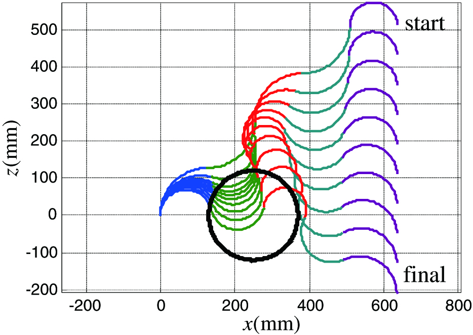Fig. 4. Linear trajectory control of a five-segment continuum manipulator without considering a static obstacle.

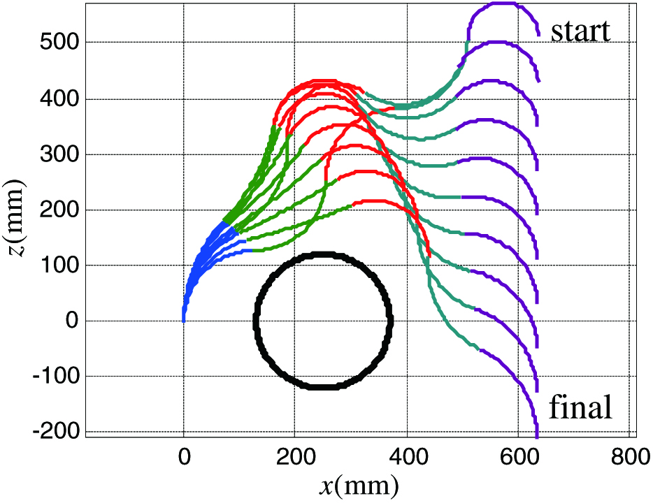Fig. 5. Linear trajectory control of a five-segment continuum manipulator with considering a static obstacle.

Furthermore, a six-segment continuum manipulator passing through a tight space between multiobstacles is also presented in Fig. 6. In this numerical simulation, the single intermediate characteristic point is selected to be the origin of the base frame of the last segment. By selecting a proper scale factor $α_{1}$ , the six-segment continuum manipulator passes through the gap between the three obstacles while the orientation of the end-effector remains unchanged, which is similar to the operation tasks illustrated in Figs. 4 and 5.

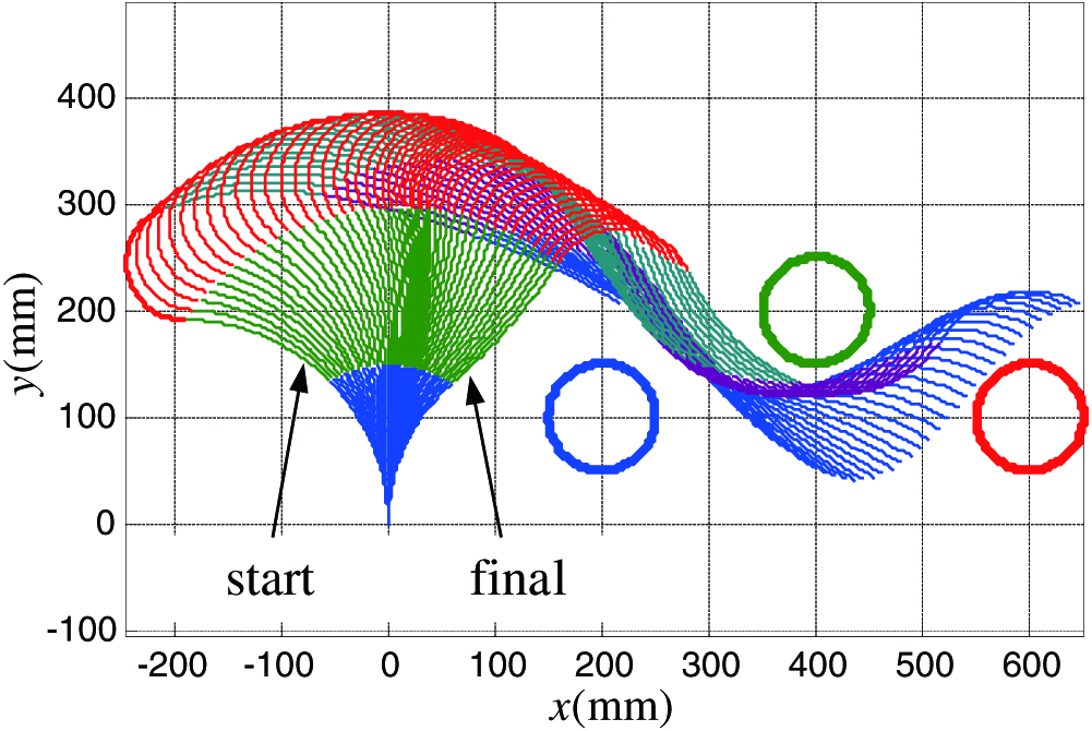Fig. 6. Curve trajectory control of a six-segment continuum manipulator with considering three static obstacles.

V.CONCLUSIONS

By applying exponential coordinates based on the Lie group theory, this paper presented a complete kinematics modeling process for the tendon driven continuum manipulators and a novel motion planning method—DCM—for the hyper-redundant continuum manipulators. The remarkable features of the present motion planning approach included: it was a motion plan method in global task space; it did not require any optimization index made up of convex functions; it did not require the task space to be a convex space; and the method provided a very flexible way of realizing the target motion optimization by dynamically adjusting the scale factors of the free velocity vectors.

Kinematics Modeling and Motion Planning of Tendon Driven Continuum Manipulators

I.INTRODUCTION

II.KINEMATICS MODELING OF A CONTINUUM MANIPULATOR WITH PIECEWISE CONSTANT CURVATURES

A.THE KINEMATICS MODELING FROM CONFIGURATION SPACE TO TASK SPACE

B.THE KINEMATICS MODELING FROM ACTUATION SPACE TO CONFIGURATION SPACE

III.DIFFERENTIAL KINEMATICS OF THE CONTINUUM MANIPULATORS

IV.MOTION PLANNING OF THE CONTINUUM MANIPULATORS

V.CONCLUSIONS

ACKNOWLEDGMENT

REFERENCES