I.INTRODUCTION
One of the key decisions in cell production is the timing of components in each cell. In cellular manufacturing (CM) scheduling, a set of components must be processed in cells by a set of machines [1]. The goal is to find the sequence of performing pieces in each group and the sequence of performing groups of pieces in cells on a set of machines; in such a way that the desired criterion is optimized in the schedule [2]. Different criteria can be considered for a cell production scheduling problem that can be minimized to completion time, minimum weighted total completion time, minimized maximum delay, minimized total delay, minimized total weighted delay, minimized number of delayed tasks, and minimized the number of intercellular translocations [3]–[5]. In practice, there are various operational constraints on CM scheduling. For example, start-up times can depend on the sequence of cells. In explaining the start-up times depending on the sequence of cells, it is important to note that in the cell production system, the start-up cost of machines varies according to the sequence of the family of pieces belonging to each cell.
Most algorithms developed for the group scheduling problem have two steps: the first step determines the sequence of pieces in groups and the second stage determines the sequence of performing groups of pieces in cells [6]. In terms of the number of cells, articles can be divided into two categories: articles that consider one cell and those that consider more than one cell.
The difference between the model presented in this paper and other studies is considering cell start-up-dependent start-up times with the two objectives of minimizing the total time of pieces completion and transitions between cells to determine the sequence of pieces in each cell and the sequence of groups of pieces in cells. Simultaneously presenting a multi-criteria mixed integer programming model. This study presents a new mathematical model for the design of reliable CM systems (CMS), which leads to reduced manufacturing costs, improved product quality, and improved total reliability of the manufacturing system.
The rest of this paper is organized as follows: Section II discusses related works to scheduling problem in CMS. Section III presents details of the proposed method to solve the CMS problem. The experimental results and discussions of the proposed method are reported in Section IV. Section V presents conclusions.
II.RELATED WORKS
Various studies have been conducted in which attempts are made to develop innovative algorithms to solve the problem of cell production scheduling, some of which are analyzed below.
In [7], several cells are considered and an innovative method for minimizing the completion time is presented. In [8], an algorithm for optimal solution of the workshop flow scheduling problem of two machines is presented, at which the start-up is considered. In [9], the workshop flow problem of two machines was timed with start-up time. In [10], they considered the issue of workshop flow scheduling in which each group needs start-up time and harvest time from the same machine. In [11], A. Adinarayanan et al. define the lower limit for optimizing the total construction time and propose the branch and limit method for achieving the optimal sequence of pieces and groups. Given that scheduling cell production systems is a difficult indefinite polynomial problem.
In [12], the problem of cell scheduling with one cell, several machines and sequence-dependent preparation time was considered with the aim of minimizing the total construction time and ignoring intercellular movements. Scalar solved the problem with improved innovative algorithms. Here, the problem is solved with genetic and mimetic meta-heuristic algorithms, and also the problem is solved with the meta-heuristic forbidden search algorithm. In [13], the problem of scheduling cell production with the aim of minimizing the time of completion of pieces and intercellular displacements has been solved with the mimetic algorithm.
In [14], studies were performed on the implementation of different methods resulting from a crossover of three methods PT (Petrov, 1966), LN (Logendran and Nudtasomboon, 1991), and CDS (Campbell, Dudek and Smith, 1970), and in the end it was stated that the LN–PT method, in which the LN method was used in the first stage and the PT method in the next stage is superior to the combined methods of PT–LN, PT–CDS, and CDS–PT. The PT and CDS algorithms are single and multiple innovative algorithms, respectively, which simplify the workflow scheduling problem with n work and m machine to problems with n work and two machines, and then use the Johnson algorithm to sequence tasks.
Layout design is the process in which industrial robots and other manufacturing system components are allocated at specific positions so that the assembly tasks can be handled appropriately. In [15], developed a tool for optimizing assembly work cell layout using simulated annealing algorithm. This method yields several possible and optimal positions for a machine, and several layouts are thus obtained at the end of execution. In [16], proposed a heuristic algorithm to optimize the layout of a robot work cell. These methods require explicit constraint handling regarding component overlapping, since component coordinates are handled as design variables, and this implementation obstructs global searching of the solution space.
III.PROPOSED METHOD
During the cell production system scheduling process according to the model proposed in the paper, the expected outputs are: (i) forming a family of pieces according to the location of machines in each cell, (ii) determining the sequence of pieces for production in each cell, and (iii) sequencing of groups of components in cells.
A.MATHEMATICAL MODEL
The proposed model is presented by describing the assumptions, parameters, variables, objective function, and constraints. The assumptions considered for this model are: 1) the operating time of all pieces on any type of machine is definite, 2) the number of pieces is definite and fixed, 3) the number of machines in the system is definite and fixed, 4) the number of existing cells in the system it is fixed, 5) the machines in each cell are known, 6) each type of machine can perform only one type of operation and each operation can also be performed by one type of machine, 7) the distance between the cells is the same; that is, the intercellular displacement time is fixed for all movements, and 8) we will not have a breakdown time for the machines, and the start-up times for each machine are specific and depend on the cell sequence.
As we know, in a general approach, several criteria should be considered in scheduling; that is, all the criteria for scheduling cell production must be combined in a way that functions in the objective function. But due to the complexity of the problem and the problems arising from the computational time required; it is not possible to consider all of them. Therefore, in this paper, only the total construction time (completion of pieces or tasks) and intercellular movement will be considered. The aim of the model is to minimize the total manufacturing time and intercellular movement time.
The following are the indices and parameters of the cell production problem. Here, i is the symbol of the pieces that belong to the set i = {1,…, P}, and P is the number of pieces. j is the machine symbol that belongs to the set j = {1,…, M}, and M is the number of machines. c is the symbol of the cell that belongs to the set c = {1,…, f}, and f is the number of cells. k is the symbol of the sequence of pieces that belongs to the set k = {1,…, K}, and K is the number of sequences. b is the symbol of the cell sequence that belongs to the set b = {1,…, KC}, and KC is the number of sequences.
The values of the input parameters that must be specified at the beginning of solving the mathematical model are: component manufacturing path, operating time, machine placement in the cell, intercell movement time, and sequence-dependent start-up time. Here, tij is the time required to process piece i on machine j, and aij and mjc are defined as follows:
In addition, sncj is the start time on machine j in cell c when it is immediately after cell n, and sccj is the start time on machine j in cell c.
In addition, decision variables are summarized as follows:
In addition, Ckjcb was the construction time of the piece in sequence k on machine j in cell c, which is in sequence b, and Cmax was the total construction time.
The objective function is to minimize intercellular movement time and total manufacturing time. In fact, the model considers the problem both in terms of timing and operation.
Assigns each component to a cell according to (7).
Where, (8) ensures that each sequence is assigned only one cell.
Where, (9) ensures that each cell is assigned to only one sequence.
Where, (10) assigns each of the components assigned to each cell to a sequence in that cell.
Where, (11) ensures that each sequence in a cell is assigned to a maximum of one piece.
Equates the completion time of the piece assigned to the first sequence on the first machine in the cell in the first sequence to the sum of the specified processing time of the piece and the start-up time of the specified cell on the first machine.
In this regard, completes the time assigned to the k-th sequence on the first machine in the cell in the first sequence if the piece in our sequence is preceded by the specified cell (for the first machine is set up in the desired cell) equal to the sum of the completion time in the previous sequence and the processing time in the current sequence; otherwise, it is equal to the sum of the current sequence processing time and the start time of the first machine in the specified cell.
Equates the completion time of the piece allocated to the first sequence of cells in sequences other than the first sequence on the first machine with the sum of the completion time in the last sequence of the previous cell and the start-up time of the first machine in the sequence cell. The current and processing time of the piece puts the first sequence of the current cell.
Equals the completion time of the piece allocated to the k sequence on the first machine in a cell that is in sequences other than the first sequence equal to the sum of the completion time of the previous sequence and the processing time of the piece specified in the current zinc sequence. The first machine and if there are no pieces in the current sequences in the specified cell in the specified cell, the preparation time of the first machine in the cell is considered.
Equals the completion time of the piece allocated to the first sequence on machine j in the cell assigned to the first sequence equal to the total completion time of this piece on machine (j − 1) in the same sequence and start-up time of machine j is specified in the cell and the processing time of the sequence piece k is placed on machine j.
Equals the completion time of the piece allocated to the first sequence on machine j in the cell assigned to the sequence other than the first sequence equal to the sum of the maximum completion time of this piece on the previous machine (j − 1) in the current cell and the completion time of the last sequence of the previous cell (b−1) on machine j with the start time of machine j in the current cell with the processing time of the first sequence piece in the current cell (b) on machine j.
In this regard, sets the completion time of the piece assigned to the k sequence (other than the first sequence) on machine j in the cell in the first sequence if specified before the piece; the piece is located in the sequences before (d < k) of the specified cell (for machine j the start-up is done in the desired cell) equal to the sum of the maximum completion time of the previous sequence (k − 1) on machine j and the completion time of the current sequence (k) on the previous machine (j − 1) with the processing time in the current sequence on the machine j and otherwise equal to the sum of the maximum completion time of the previous sequence (k − 1) on the machine j and the completion time of the current sequence (k On the previous machine (j − 1) with the start time of machine j in the first sequence cell with the processing time in the current sequence on machine j.
Equals the completion time of the piece allocated to sequence k on machine j in cell c, which is allocated to sequence b. The sum of the maximum completion time of the previous sequence (k − 1) on machine j and the total completion time of the current sequence (k) on the previous machine (j − 1) with the processing time of the specified piece in the current sequence on machine j and if no interrupts in previous sequences If the current sequence (d < k) is not in the current sequence cell, it sets the start time of machine j in the objective cell.
Accordingly, (12) Cmax equals the maximum completion time.
Where, in (13), values 0 and 1 are introduced.
B.PROPOSED GENETIC ALGORITHM
Genetic algorithm is a comparative stochastic search approach based on Darwin’s theory of proportionality. The most suitable organ has the highest probability of survival and consequently an increase in number; while the most unworthy die. One of the most important features of GA is its tendency toward definite or near-optimal optimal solutions even in large or complex search spaces. Fig. 1 shows the general method of genetic algorithm.
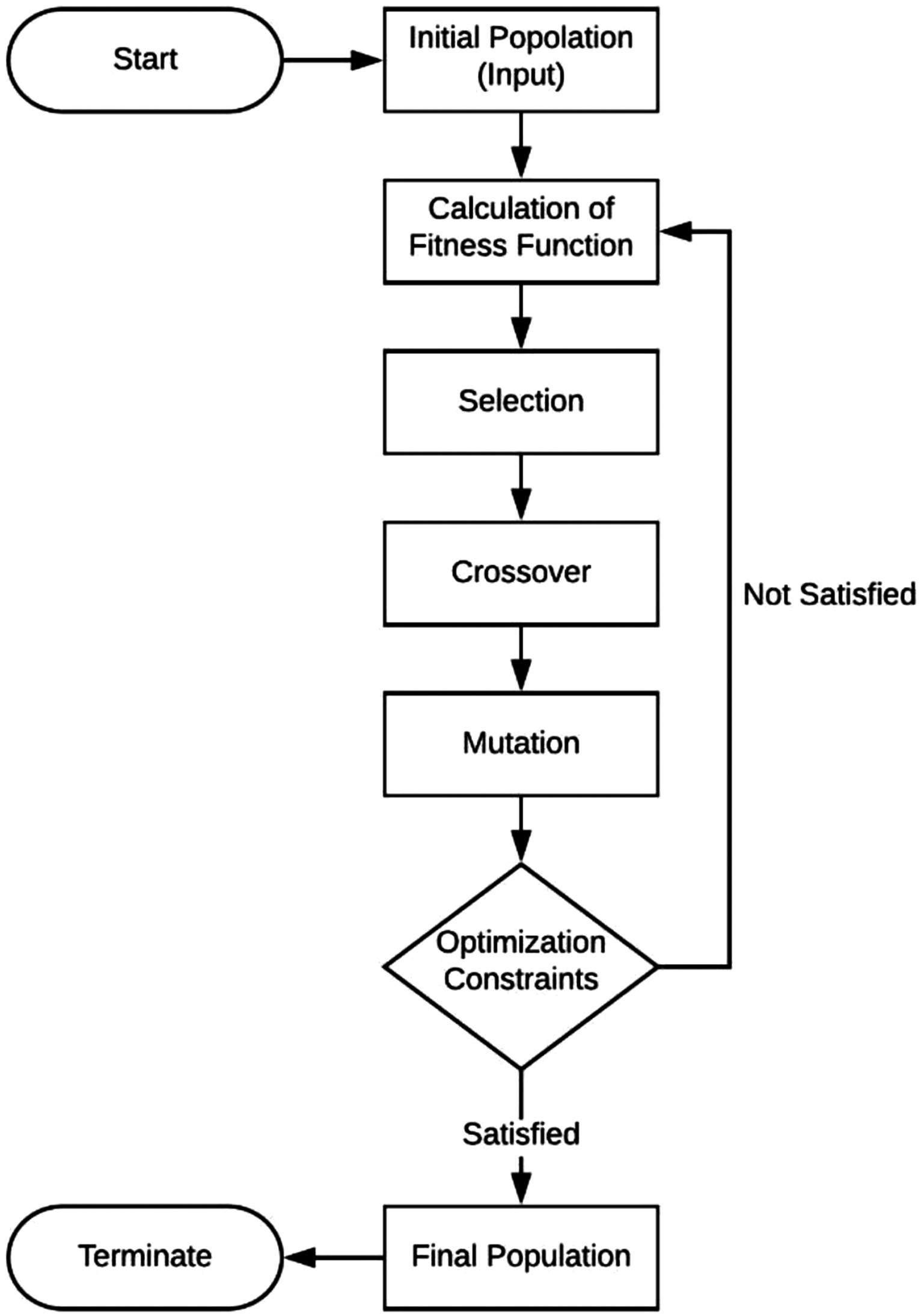 Fig. 1. Overview of genetic algorithms.
In this problem, matrix A with dimensions (c × p) is designed as a solution for sequencing pieces in cells. Thus, in p, the element of this matrix is assigned numbers from 1 to p, and how to design this matrix and the solutions is such that the solutions are all created as possible and the problem does not go in an impossible environment.
As stated earlier, to minimize the total construction time, we are faced with two types of sequences: sequencing of pieces in each cell and sequencing of cells, which are determined simultaneously. So corresponding to each sequence of components inside the cells, we will also have a sequence for the cells. Therefore, corresponding to matrix A, which specifies the sequence of pieces in cells, matrix B is considered to have dimensions (c × 1), in each row of which the sequence of cells is given. So at the end of each matrix A and one matrix B is a solution for the model presented in Piece 2. Fig. 2 shows an example of a chromosome for 10 pieces and 3 cells.
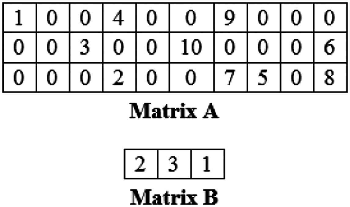 Fig. 2. Example of a proposed chromosome.
In this example, the two matrices A and B together are a chromosome that shows the pieces (1,4,9) to the first cell, the pieces (3,10,6) to the second cell and the pieces, respectively. (2,7,5,8) are assigned to the third cell, respectively, and also the sequence of cells is 2, 3, and 1: that is, first the components in the second cell are processed in the specified sequence; then, the pieces in the third cell and at the end of processing the pieces related to the first cell are done.
The first step in determining how to turn each answer into a chromosome is to create an initial population of chromosomes. At this stage, the initial answer is generated randomly.
If g is the value of the objective function obtained from (6), by performing conversion (14) we obtain the value of the fitness function for each of the chromosomes produced in the previous step:
Where, n = popsize. There are several ways to select Cmax; the largest gi value ever seen is the largest in the current population or the largest in the previous generation k. Here, the value of Cmax is equal to the largest value of g in the current population.
The mechanism of production and the ambiguity of how chromosomes are selected from the sampling space are related. In this paper, the method of random sampling with placement was used. In this method, the probability of selection corresponding to each chromosome is calculated based on its suitability; so if fk is the suitability value of the k chromosome, the probability of survival corresponding to that chromosome is,
Selection method: The main selection method is the roulette wheel [17]. In this method, in order to select each chromosome, first a random number between zero and one is generated, and then the said number in each interval is selected; the corresponding chromosome is selected. The selected chromosome is returned to the chance wheel, and this cycle continues until the required population size is selected.
Crossover rate (CP) is the probability of the crossover operator occurring on each of the chromosomes. For each chromosome, it generates a random number between zero and one. If this number is less than CP, the chromosome is selected for the crossover. In this case, as described below, it produces a new child; otherwise, the desired chromosome is not selected for the operation of the crossover.
Crossover operators are operators that select one or more points from two or more answers and swap their values. These operators consider an answer, do not replace pieces of the answer with other answers, and create new answers. In this paper, a point operator is used to produce offspring, which is randomly identified as a point of incision, and from this point of incision, the right side of the parent chromosomes are swapped; in this way, two new children are born. The children created may be an unjustified solution, in which case the two children created must be justified as two solutions to the problem. An example shows how the designed crossover operator works, which considers a matrix A with 5 components and 2 cells. The two chromosomes P1 and P2 are the parents that are produced after the cutting operation of two children C1 and C2. Fig. 3 shows an example of a crossover operator.
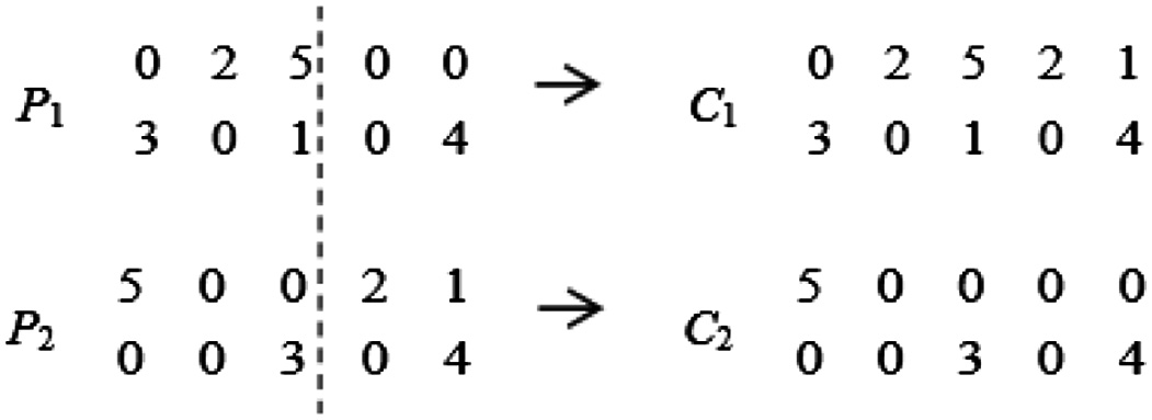 Fig. 3. Example of a crossover operator.
The mutation operator is used to prevent the search from diverging in a local optimization. The probability or rate of mutation (MP) in a chromosome is equal to the probability that each of the genes will change, which is a small amount. If this number is less than MP, the mutation is performed as described below; otherwise, it remains unchanged. In the chromosome selected for the mutation, two random numbers between one and the total number of genes are selected and the values The genes corresponding to these numbers are interchanged, and the offspring may be an unjustified solution, in which case the two offspring should be justified as two solutions to the problem.
Consider chromosome C1 in the previous example; suppose locations 3 and 4 are selected as mutation sites; as a result, it converts to C′1 after the mutation. Fig. 4 shows an example of a mutation operator.
 Fig. 4. Example of a mutation operator.
Another discussion in the implementation of genetic algorithms is how to deal with the limitations of the problem, because the genetic operators used in the algorithm produce unjustified chromosomes. In this paper, a modification strategy is used that in this method, instead of deleting the unjustified chromosome, it becomes a justified chromosome. This operation is used after the crossover operation, which may create unjustified chromosomes.
Corresponding to each of the unjustified chromosomes, we define two transfer matrices, all of whose strands are zero at the beginning. We compare the genes on the left side of the unjustified chromosome with the genes on the right side of the cutoff point; for each equation we observe, we zero the corresponding gene on the corresponding chromosome and its corresponding value in the transfer matrix. We do this for all the genes to the right of the cutoff point. Finally, to produce the justified child of the first parent, we use the transfer matrix of the second parent, and vice versa; in this way, we use the corresponding transfer matrix values for the genes to the right of the cutoff point. In this way, children try to inherit their parents’ traits, rather than eliminating them by deleting unwarranted chromosomes. Consider the previous example to clarify the matter; for two chromosomes C1 and C2 we have two matrices I1 and I2. Finally, by inserting matrix I1 in chromosome C2 and matrix I2 in chromosome C1, two justified children C'1 and C'2 are produced. This process is shown in Fig. 5.
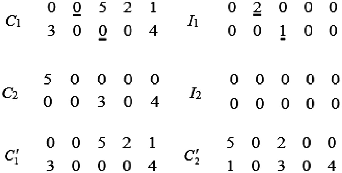 Fig. 5. Example of a strategy for dealing with constraints.
The movement of the genetic algorithm from one generation to the next, that is, the process of selecting the correct chromosomes and reproducing, continues until the criterion of cessation is satisfied. Several cessation criteria can be selected, including the fixed number of generation generation, computational time, and convergence of fitness functions. In this paper, a fixed number of generation generation is used as a criterion for termination of the proposed algorithm.
IV.RESULTS AND DISCUSSION
In this section, the performance of the proposed algorithm to improve the workshop production planning systems using the P-FJSP dataset from the UCI machine learning repository is evaluated. The simulation is done with MATLAB software version 2019a and NSGA-II and NRGA algorithms are used for comparison work. In all experiments, an average of 15 distinct implementations of the algorithms are reported to ensure results.
The value of the parameters used in the simulation of the proposed algorithm is as follows: population size: 50, crossover operator rate: 0.85, mutation operator rate: 0.15, and number of generations: 500.
Quality, scatter, distance, and time indices are used to evaluate the performance quality of the proposed algorithm with four-objective function [18]. The quality index tests the uniformity of the distribution of Pareto archives obtained at the boundaries of the solutions. This index is defined as (16).
Where, di represents the Euclidean distance between two adjacent non-defeated solutions in the Pareto archive. is the mean of di, and N represents the number of members in the Pareto archive list.
Dispersion index shows the amount of variation that exists between the data of a distribution [19]. This index is used to determine the amount of unsuccessful solutions in the Pareto archive on the optimal boundary. This index is defined as (17).
Where, Euclidean distance between two adjacent solutions and on the optimal boundary.
The scatter criterion represents the Euclidean distance between the first and last solution in a Pareto archive, and the higher the variability values, the greater the quality of the results [20]. The distance index is used to show the compatibility of the distance between solutions in the Pareto archive. Lower values of the distance criterion indicate that the stability of the distance between the solutions is higher. This index is defined as (18).
Where, di represents the Euclidean distance between the two non-defeated solutions in the Pareto archive, where makespan is 1 and stability is 2. The last criterion used for comparison is runtime. Since all the parameters in the algorithms are the same, this criterion is a suitable comparison index for evaluating the production planning system.
In this paper, P-FJSP dataset has been used to evaluate the proposed algorithm and make comparisons. This dataset was produced by Brandimart (1993) and includes 10 samples [21]. The parameters of each of the problems in this dataset are generated randomly using a uniform distribution between the two limits [22], [23]. The number of tasks is defined from 10 to 20, the number of machines from 4 to 15, the number of operations for each task from 5 to 15, and the number of operations for all tasks from 55 to 240. In addition, it is specified what machines are needed for each job.
NRGA and NSGA-II algorithms have been used for comparison work according to the criteria of scatter, distance, quality, and execution time (s). Comparison of scatter criteria in different algorithms on 10 experimental samples is shown in Fig. 6. The results show that the NSGA-II algorithm has a better quality than the NRGA. On the other hand, the proposed algorithm with a scattering index of 74.85 has better performance than both methods.
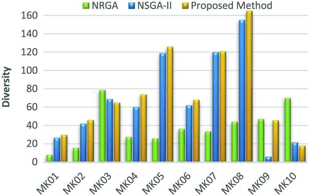 Fig. 6. Comparison of different methods in the diversity criterion.
Fig. 7 shows the comparison results in the distance criterion. Because lower values of distance mean high quality, in the MK09 and MK10 samples the NRGA method performs better than the NSGA-II. However, on average, the distance index in NRGA and NSGA-II algorithms is 19.19 and 12.71, respectively, which indicates the production of better solutions by NSGA-II algorithm. Despite the superiority of the NSGA-II algorithm over the NSGA, the proposed algorithm with an average distance index of 12.4 has better performance than both methods.
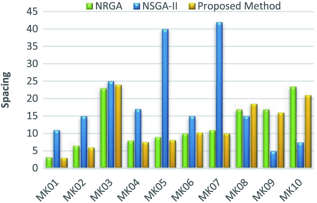 Fig. 7. Comparison of different methods in the distance criterion.
The NSGA-II method is superior to the NRGA method in all samples except MK08 based on the quality index. In this criterion, the superiority of the proposed method in comparison with the NSGA-II method is present in all samples and as a result; it shows a better quality of performance. Fig. 8 shows the average results of comparing the quality index.
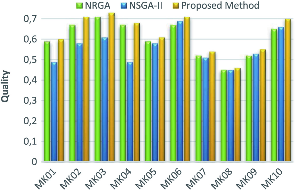 Fig. 8. Comparison of different methods in the quality criterion.
In general, the proposed method has a better performance in dispersion index than MKR3, MK09, and MK10 in other samples than NRGA and NSGA-II methods, and the dispersion index has an average of 19 in these two methods, respectively. /36 and 96/8 units have increased. The reduction of distance index in the 10 samples tested decreased by 7.05 and 0.57, respectively, in contrast to NRGA and NSGA-II methods. The results of the proposed method have a good performance in the quality index and on average; this index has increased compared to the two compared methods by 0.01 and 0.11, respectively. Due to the use of all three methods compared to the genetic algorithm, the results in the runtime criterion fluctuate in almost the same range. The average results of this criterion for the proposed method and the two methods NRGA and NSGA-II are 2965, 3015, and 2931 s, respectively, which is a relative advantage for the proposed method.
V.CONCLUSION
The model proposed in this paper was a definitive model for minimizing idle time and assigning pieces to cells by taking cell sequence-dependent start-up times to minimize the time required to complete pieces and intercellular movement. According to studies, this problem is of the indefinite polynomial type, which can be solved by increasing the number of pieces and machines through optimization software. Approaches such as branch and limit and dynamic programming with increasing the number of tasks have limited computation time and limited storage on the computer; therefore, the use of innovative and meta-heuristic algorithms can be effective. Genetic algorithm is one of the most important meta-heuristic algorithms that is used to optimize various functions. A genetic algorithm is a search algorithm that searches for an answer in an area and mimics biological evaluation processes. The genetic algorithm according to the characteristics described was used to solve the problem in this paper.