JAIT

I.INTRODUCTION

The conventional offline optical character recognition (OCR) algorithm has been a hotspot in the field of pattern recognition. It consists of four steps, including character image preprocessing, text line segmentation, character segmentation, and character recognition. With the development of machine learning, some brilliant classification algorithms [1–6] are good enough for single character recognition. Thus, the key step for good recognition results is text segmenting in segmentation-based algorithms. Several researches were proposed to settle the character segmentation problem. The connected-component algorithm [7] has good performances in the non-torched field but cannot nicely split the torched character images. Viterbi-based algorithm [8] and the dripping segmenting algorithm [9] had done well in this task, but both were prone to unsolvable over-segmentation problems. Some other attempts have been made to address this problem by using language model-based recognition algorithms [10–13]. They tried to improve the recognition performances by integrating predefined language models into recognition algorithms. However, the predefined language models usually only considered the short-distance history characters ignoring the long term. The torched-stroke and over-segmentations still affect the performances of the existing segmentation-based OCR algorithms.

Given that, an idea of “segmentation-free” recognition, called sequence labeling as shown in Fig. 1, was given significant attention. In sequence labeling, a text line image can be directly converted to a label sequence. T. H. Su [14] proposed 36DGVS algorithm based on a hidden Markov model (HMM). It used a sliding window to extract the image features of the handwritten text line and predicted the optimal recognition result by using the HMM. Afterward, with the development of deep learning, some sequence labeling architectures [15,16] based on deep learning were used for sequence prediction. However, these algorithms assumed the pre-extraction features as network inputs which became the new problem of the sequence labeling algorithm.

Fig. 1. Sequence labeling.

Thereby, some end-to-end algorithms [17–21] were proposed to convert inputs of text line images into outputs of label sequences without the pre-extraction features. The convolutional recurrent neural network (CRNN) [19] succeeded in English text sequence labeling. However, it was prone to the over-fitting problem in some situations with a large alphabet or small databases.

Thus, a sequence labeling algorithm is proposed with the following contributions.

(a)An improved network based on the CRNN, consisting of four neural network layers, is proposed to deliver better performances and more efficiency in handwritten sequence recognition.
(b)A novel databases uniform method, based on data filling, is proposed to normalize the databases into uniform size for better model training.
(c)Handwritten recognition experiments in multiple languages are carried out in order to test the robustness network.

The rest of the paper is organized as follows. Section II presents the proposed algorithm. Section III introduces the experimental environment and databases used in this paper. Four networks based on the proposed algorithm with different parameters and experimental results are discussed in detail in section IV. Section V gives a conclusion.

II.THE PROPOSED ALGORITHM

The architecture of the proposed network consists of four neural network layers, including preprocessing, CNNs, BDLSTM, and CTC loss layers as shown in Fig. 2. The preprocessing layer is used to convert the image into a normalized binary image, which will be further discussed in the experimental databases section. The designed CNNs are used for spontaneous feature extraction and image dimensionality reduction in the second layer of the proposed algorithm. The BDLSTM layer follows the CNNs to predict the sequence output based on the contextual information. The CTC loss layer is used for the alignment between sequences and labels, and the backward of the loss at the end of the network.

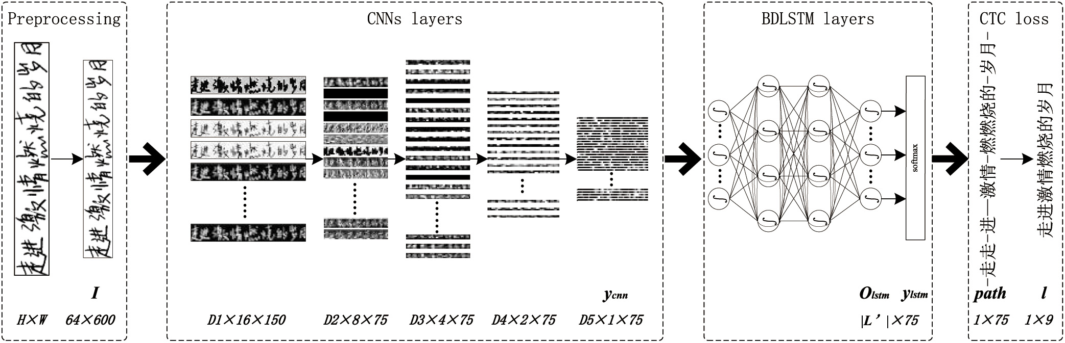Fig. 2. Architectures of the proposed network.

A.CNNs LAYER

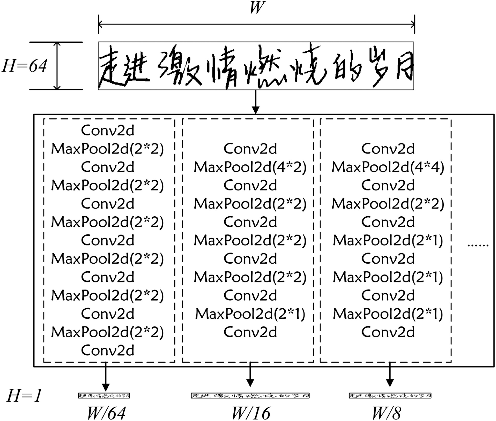
The CNNs layer, used for feature extraction and image dimensionality reduction, includes several convolutional layers and pooling layers but excludes the fully connected layers that are used in the common CNNs to retain the structure information of the input images as completely as possible. Thus, the architecture of the CNNs layer should be designed reasonably by meeting the following two requirements.

(1)The height of CNNs layer outputs: H = 1.
(2)The width of CNNs layer outputs: W≥5×label length.

On that foundation, the outputs of CNNs layer can fit the input dimensional requirements of the BDLSTM layer and retain the structure information at the same time. Suppose that the height of the preprocessed image is H = 64, the architecture of CNNs and pooling layers in this paper should be designed as shown in Fig. 3.

Fig. 3. Parameters setting of CNNs and pooling layers.

B.BDLSTM LAYER

The designed CNNs layer will produce a feature vector with structure semantics, which is invaluable for label prediction. Some networks are good at label prediction. Recurrent Nueral networks (RNNs) [6] do well in sequence prediction using the information about the long past inputs. Moreover, the bidirectional recurrent neural networks (BDRNNs) [22] can make good use of both past and later inputs. Based on BDRNNs, it is possible to predict the labels with a suitable feature vector produced by the CNNs layers mentioned above.

However, it is difficult to train the BDRNNs, and it is impossible to retain information for a long period because of the evaporation of gradient information or large increase along the time delay, called the vanishing gradient or the exploding gradient problem [23,24] as shown in Fig. 4(a) in BDRNNs network. Meanwhile, the long-short term network (LSTM) [25] is a variant of RNNs, which can tackle the problem in RNNs effectively.

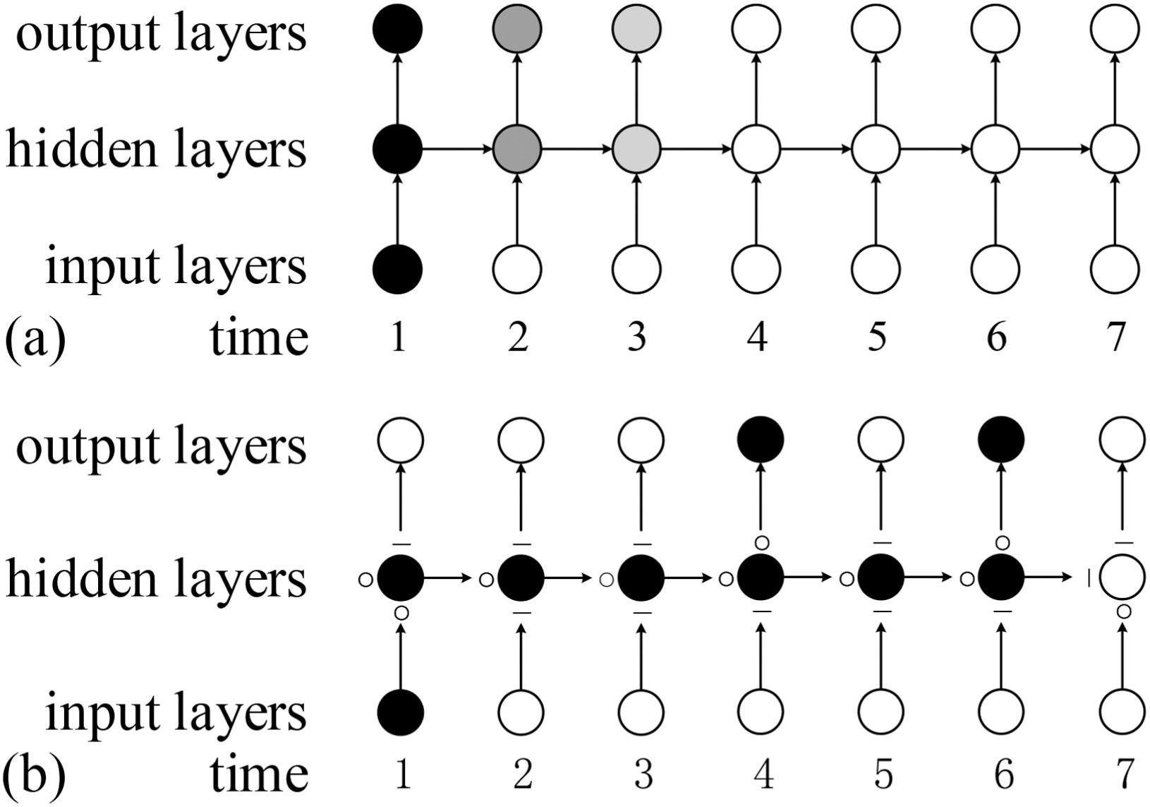Fig. 4. Vanishing gradient problem: (a) gradient transfer of RNNs and (b) gradient transfer of LSTM.

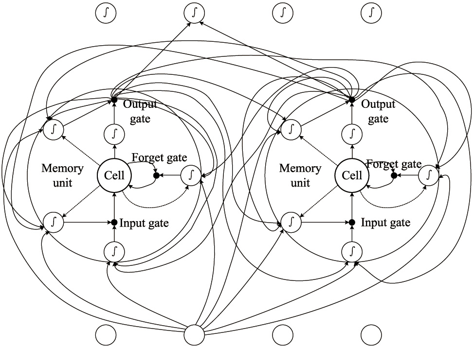
The main idea of LSTM is to replace the basic unit in RNNs with a memory unit containing one or more self-connected memory cells and three gates. It is quite feasible to use the long-term information about input sequences to predict labels. The gradient transfer in RNNs and LSTM are shown in Fig. 4(b) corresponding to Fig. 4(a).

Moreover, BDLSTM network, as shown in Fig. 5, are good at using long-term information of past and later input sequences.

Fig. 5. BDLSTM network.

From then on, suppose that a neural network consists of CNNs, BDLSTM layers described above, is with a part of input image shown in Fig. 1, it will produce results of “rroouunndd” or “roundd,” or other possible outputs for the ground truth “round” for the reason that the output of the current network cannot align with the ground truth correctly.

C.CTC LOSS LAYER

CTC [26] proposed by Graves for labeling the unsegmented sequences can solve the alignment problem of sequence prediction in this paper. Suppose that there is a letter set $L$ , for instance, the letter set for English letters is $L = {A, \dots, Z, a, \dots, z}$ and length of the set is $| L | = 52$ . The letter set for the CTC algorithm should be $L^{'} = L \cup {-}$ where “ $-$ ” represents a blank character and $| L^{'} | = | L | + 1$ . The relationship between the inputs and labels of the CTC algorithm can be expressed by $f_{c t c}$ as shown in formula (1):

f_{ctc} (- AABB -) = f_{ctc} (- AA - B -) = AB

(1)

From that, the inputs of the CTC algorithm will be compressed with designed rules. The blank character “ $-$ ” plays a key role in the rule. It makes correct results in some situations as shown in formulas (2) and (3).

(a)If there is a “ $-$ ”, the result is shown in formula (2):
$A - A = AA$ (2)
(b)If there is no “ $-$ ”, the result should be what is shown in formula (3):
$AA = A$ (3)

In this way, the outputs of the CTC layer can align with the label sequences.

D.THE FORWARD AND BACKWARD PROCESS

Suppose that there is an input image $I$ with a size of 64×600, the label sequence corresponding to $I$ is $l$ and the letter set is $L^{'} = L \cup {-}$ . The forward and backward of the proposed network can be expressed as follows:

1)FORWARD

(a)Image preprocessing. The input image I should be converted to a binary image and the height of the image should be resized into H = 64 for the stability and efficiency of the network. By the way, we suppose that there is one grayscale image I with a size of 64×600 as the input of the CNNs in this part.
(b)CNNs layers. The CNNs layer is represented with a symbol $f_{c n n}$ . The forward pass of CNNs layers is expressed by formula (4):
$y_{cnn} = \underset{θ_{1}}{f_{cnn}} (I)$ (4)
where $θ_{1}$ represents the parameters in CNNs layers and $y_{cnn}$ represents the feature vector outputs as the output of the CNNs layer. The CNNs layer shown in Fig. 2 is corresponding to the third structure described in Fig. 3. Through CNNs layer, the image I will be transformed into a feature vector $y_{cnn}$ with a size of D5×1×75 by the CNNs layers as shown in Fig. 2.
(c)BDLSTM layers. The BDLSTM layer is represented by $f_{l s t m}$ . The main task of the BDLSTM layers is to predict the label sequence $y_{lstm}$ based on the feature vector $y_{cnn}$ . The forward pass of BDLSTM layers can be expressed as formulas (5) and (6):
$O_{lstm} = \underset{θ_{2}}{f_{lstm}} (y_{cnn})$ (5)
$y_{lstm} = Softmax (O_{lstm})$ (6)
where $θ_{2}$ represents the parameters in BDLSTM layers and $O_{lstm}$ , with a size of $75 \times | L^{'} |$ , determines the output of the BDLSTM networks. The output should be sent to a $S o f t m a x$ layer to obtain the posterior probability vector $y_{lstm}$ of the label sequence prediction, with a size of $75 \times | L^{'} |$ , as given in formula (6).
(d)CTC loss layer. The optimal label sequence prediction $l^{'}$ of the input image can be estimated by the posterior probability vector $y_{lstm}$ based on CTC loss layers (represented by $f_{c t c}$ ) using formula (7):
$l^{'} = Softmax (O_{lstm})$ (7)

2)BACKWARD

Backpropagation through time algorithm (BPTT) by Werbos [27] is used to train the proposed networks in this paper. In addition, to finish the training of networks in an end-to-end manner and tackle the alignment problem of sequence prediction, the CTC loss is provided behind the $S o f t m a x$ loss layer. Suppose that there is a ground truth dataset composed of a group of handwritten images I labeled correctly with label sequences l. The dataset is determined by D as given in formula (8):

D = {(I_{1}, l_{1}), (I_{2}, l_{2}), \dots, (I_{N}, l_{N})}

(8)

The CTC loss represented by loss can be calculated using formula (9):

loss = - lnp (l | y_{lstm}) = - ln \sum_{path} \prod_{T} {y_{lstm}}_{path}^{t}

(9)

Then, the loss of backpropagation to BDLSTM layers can be calculated with the chain rule based on the back propagation through time (BPTT) algorithm as shown in formula (10). Each partial derivative in formula (10) can be calculated based on the formula derivation by Graves [26]:

\frac{\partial loss}{\partial θ_{2}} = \frac{\partial loss}{\partial y_{lstm}_{path}^{t}} \frac{\partial y_{lstm}_{path}^{t}}{\partial O_{lstm}_{path}^{t}} \frac{\partial O_{lstm}_{path}^{t}}{\partial θ_{2}}

(10)

Similarly, the loss of backpropagation to CNNs layers can also be calculated with the chain rule as shown in formula (11):

\frac{\partial loss}{\partial θ_{1}} = \frac{\partial loss}{\partial O_{lstm}_{path}^{t}} \frac{\partial O_{lstm}_{path}^{t}}{\partial h_{N}} \frac{\partial h_{N}}{\partial h_{N - 1}} \dots \frac{\partial h_{1}}{\partial y_{cnn}} \frac{\partial y_{cnn}}{\partial θ_{1}}

(11)

where

h_{N}

represents the parameters of the hidden layers N of BDLSTM networks. Once the iteration of network training based on one input image is done, the network will converge after some epoch of iterations in the best case.

III.EXPERIMENTAL ENVIRONMENT AND DATABASES

A.EXPERIMENTAL ENVIRONMENT

The experimental results in this paper are all based on a desktop PC with an Intel(R) Core(TM) i9-10850K CPU, 16GB memory, and an NVIDIA GeForce GTX 1080 with 8GB memory.

B.EXPERIMENTAL DATABASES

To evaluate the effectiveness of the proposed algorithm, six typical offline handwritten databases were used for the experiments, including the handwriting database by Institut für Informatik und angewandte Mathematik (IAM) [28] for English, the handwriting database by Institute of Automation Chinese Academy of Sciences (CASIA-HWDB) (including unconstrained text lines (HWDB2.0-2.2) [29] and the Harbin Institute of Technology-Multiple Writers Database (HIT-MW) [30] for Chinese, the DigitalPeter database [31] for Russian, the Rodrigo database [32] for Spanish, and the Arabic Offline Handwritten Text Database (KHATT) [33] for Arabic. All of the databases were correctly labeled. Figure 6 shows some samples from the databases, while Table I lists the properties of the six databases.

Fig. 6. Samples of the six databases. (a) IAM, (b) CASIA-HWDB, (c) HIT-MW, (d) DigitalPeter, (e) Rodrigo, and (f) KHATT.

Table I. Properties of the six offline handwritten databases

Databases		Writers	Pages	Text line images	Alphabets
IAM		657	1,539	13,353	80
CASIA-HWDB	HWDB2.0	419	2,092	20,495	2073
	HWDB2.1	300	1,500	17,292
	HWDB2.2	300	1,488	14,443
HIT-MW		780	853	8,673	3047
DigitalPeter		1	662	9,694	76
Rodrigo		1	853	15,010	111
KHATT		1,000	2,000	13,435	94

For better training and testing processing, the images and labels used in this paper were normalized as follows:

(a)normalization of the image height. The height of the input image H was resized to 64 pixels for better efficiency, while the information was retained as much as possible.
(b)normalization of image width and label length. While the image height has been normalized, the image width and label length of each individual sample are different. With this, another contribution of this paper is to propose a data processing method to normalize the database into uniform size.

Taking the IAM database as an example, the label length of the samples ranges from 1 to 94 characters. In this paper, every label is normalized to the max label length of 94 characters. The common way for this task is padding “ $-$ ”. For instance, the labels of “A MOVE to stop Mr. Gaitskell from,” with the length of 34, will be normalized to new labels of “A MOVE to stop Mr. Gaitskell from $- - - - - - - - - - - - - - - - - - - - - - - - - - - - - - - - - - - - - - - - - - - - - - - - - - - - - - - - - - - -$ ” with length of 94 characters, by padding 60 “ $-$ ” characters at the end of the old labels. In the more extreme cases, a label with length of 1, there are 93 “ $-$ ” should be padded. It will pull in too much useless information which is disastrous for training. Therefore, the main idea of the data processing method in this paper is to fill the databases with existing samples instead of “ $-$ ”.

Step 1. Collect padding samples. Collecting some samples with a label length ranging from 1 to 51 characters, called padding samples.
Step 2. Get the original data size. Suppose the size of the original image I is $(h, w)$ , the length of the original label $l$ is $| l |$ .
Step 3. Find a suitable padding sample for the original data. Find a padding sample in which image $I^{'}$ with a size of $(h, w^{'})$ and label $l^{'}$ with a length of $| l^{'} |$ let $| l | + | l^{'} | = 52$ .
Step 4. Pad the original data. Produce a new image with a size $(h, w + w^{'})$ by splicing the original image $I$ with the chosen padding samples $I^{'}$ in the horizontal direction and the new label will be produced simply by string slicing.
Step 5. Normalize the image. The image is resized to a uniform size.

The data with a label length of 34 characters mentioned above can be normalized more reasonably, and the new labels of the data should be “A MOVE to stop Mr. Gaitskell from Commonwealth Relations Secretary, that they wish to be kept.” The rest of the databases used in this paper were normalized in a similar manner. Moreover, the databases were divided into three parts, including 60%, 20%, and 20% as the training, validation, and testing sets, respectively.

IV.EXPERIMENTAL RESULTS AND DISCUSSIONS

This section explains and discusses the details of the proposed network implementation. The parameters and the sizes of the output of each layer of the proposed network are described in Table II where batch size is 16 for network training.

Table II. Parameters of the proposed networks

Layers	Parameters	Size of outputs
Preprocessing	Data preprocessing	16 × 1 × 64 × 2133
CNNs	Conv(1,33,1,1)*	16 × 1 × 64 × 2133
	Conv(64,11,1,0)*	16 × 64 × 64 × 2133
	Pool(22,(2,2),(0,0))*	16 × 64 × 32 × 1066
	Conv(64,33,1,1)*	16 × 64 × 32 × 1066
	Conv(128,11,1,0)*	16 × 128 × 32 × 1066
	Pool(22,(2,2),(0,0))*	16 × 128 × 16 × 533
	Conv(128,33,1,1)*	16 × 128 × 16 × 533
	Conv(256,11,1,0)*	16 × 256 × 16 × 533
	Pool(22,(2,1),(0,1))*	16 × 256 × 8 × 534
	Conv(256,33,1,1)*	16 × 256 × 8 × 534
	Conv(256,11,1,0)*	16 × 256 × 8 × 534
	Pool(22,(2,1),(0,1))*	16 × 256 × 4 × 535
	Conv(256,33,1,1)*	16 × 256 × 4 × 535
	Conv(512,11,1,0)*	16 × 512 × 4 × 535
	Conv(512,33,1,1)*	16 × 512 × 4 × 535
	Conv(512,11,1,0)*	16 × 512 × 4 × 535
	Pool(22,(2,1),(0,1))*	16 × 512 × 2 × 536
	Conv(512,22,1,0)*	16 × 512 × 1 × 535
	Conv(512,11,1,0)*	16 × 512 × 1 × 535
BDLSTM	BDLSTM(512,512,512)	535 × 16 × 1024
BDLSTM	BDLSTM(512,512,nClass)	535 × 16 × 1024
	Softmax	8560 × $\| L^{'} \|$
	CTC loss	832 × 1

First, the preprocessing layer will transform the original image into a binary image with a size of $64 \times 2133$ and slice the original labels to the max label length. The size of outputs would be $16 \times 1 \times 64 \times 2133$ while the $b a t c h s i z e = 16$ .

Then the batches from the above layers will be processed into a feature vector $y_{cnn}$ with the size of $16 \times 512 \times 1 \times 513$ by CNNs layers. Conv and Pool mentioned in Table I represent convolutional and max pooling layers, respectively, where $C o n v (1, 3 * 3, 1, 1)$ represents a convolutional layer with a convolutional kernel of $3 * 3$ , the stride of 1, and the zero padding dimension of 1. $P o o l (2 * 2, (2, 1), (0, 1))$ represents a max pooling layer with pooling kernel of $2 * 2$ , the stride vertical of 2, the stride horizontal of 1, the vertical zero padding dimension of 0, and the horizontal zero padding dimension of 1.

Next, the prediction vector $O_{lstm}$ sized $535 \times 16 \times 1024$ is produced from BDLSTM layers with an input of feature vector $y_{cnn}$ , and the posterior probability vector $y_{lstm}$ sized $8560 \times | L^{'} |$ , where $| L^{'} |$ represents the length of Chinese letters set in the databases and can be obtained through a $S o f t m a x$ layer based on $O_{lstm}$ . $B D L S T M (512, 512, 512)$ represents a BDLSTM network with 512, 1024, and 1024 units in the input, hidden, and output layers because of its directionality, respectively.

Finally, the CTC layers would produce a label prediction sized $832 \times 1$ , where 832 is the product of the label length $| l |$ and $b a t c h s i z e$ 16.

The experimental results of training loss and testing accuracy of character correct rates (CCRs) on the six databases are shown in Fig. 7 and Table III. After 20 epochs training, the proposed algorithm obtains good performances on all databases except for the KHATT database which should be caused by the unique typography of the Arabic. Moreover, the differences in the converge speeds in Fig. 8 are produced by the variant sizes for different databases.

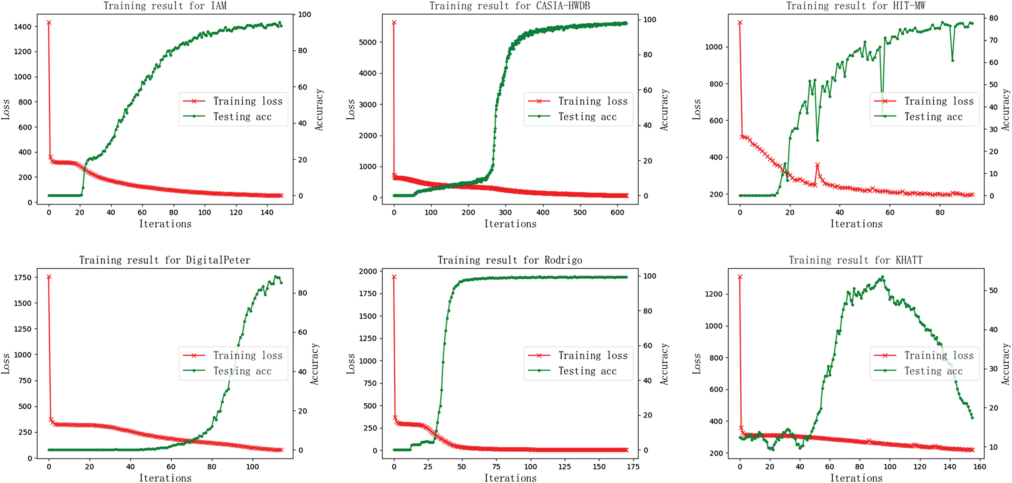Fig. 7. Analysis of experimental results on six databases.

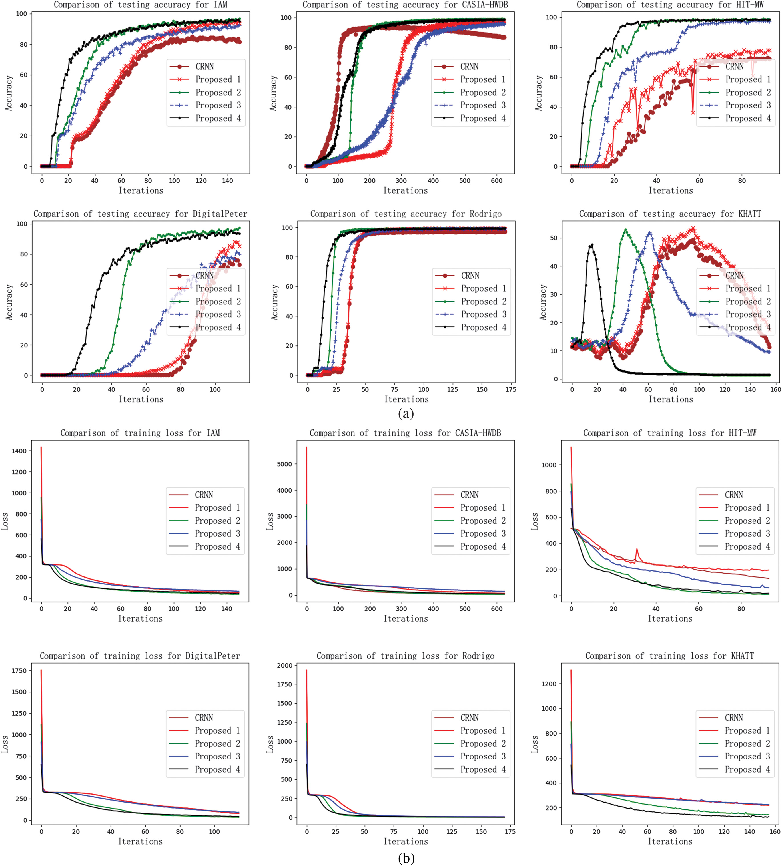Fig. 8. Comparative analysis of experimental results for the six databases. (a) Comparison of training loss and (b) comparison of testing accuracy.

Table III. Character correct rates (CCRs) on the six databases

Results	IAM (%)	CASIA-HWDB (%)	HIT-MW (%)	DigitalPeter (%)	Rodrigo (%)	KHATT (%)
CCR	96.135	97.908	77.791	88.214	99.317	58.024

Furthermore, three additional variant networks, namely Proposal 2, Proposal 3, and Proposal 4, are presented as described in Table IV based on the network in Table I called Proposal 1 hereinafter. Proposal 3 uses more suitable pooling kernels in CNNs layers, and Proposal 1 retains the structure information of the input images as much as possible and simultaneously shortens the time for each iteration. Proposal 2 and Proposal 4 use more complex BDLSTM layers by increasing the memory units based on Proposal 1 and Proposal 3 separately to improve the prediction ability of the network.

Table IV. Parameters of the proposed networks

Layers	Proposal 2	Proposal 3	Proposal 4
CNNs	Conv(1,33,1,1)*	Conv(1,33,1,1)*	Conv(1,33,1,1)*
	Conv(64,11,1,0)*	Conv(64,11,1,0)*	Conv(64,11,1,0)*
	Pool(22,(2,2),(0,0))*	Pool (44,(4,4),(0,0))*	Pool (44,(4,4),(0,0))*
	Conv(64,33,1,1)*
	Conv(128,11,1,0)*	Conv(64,33,1,1)*	Conv(64,33,1,1)*
	Pool(22,(2,2),(0,0))*	Conv(128,11,1,0)*	Conv(128,11,1,0)*
	Conv(128,33,1,1)*	Conv(128,33,1,1)*	Conv(128,33,1,1)*
	Conv(256,11,1,0)*	Conv(256,11,1,0)*	Conv(256,11,1,0)*
	Pool(22,(2,1),(0,1))*	Pool (42,(4,2),(0,1))*	Pool (42,(4,2),(0,1))*
	Conv(256,33,1,1)*
	Conv(256,11,1,0)*	Conv(256,33,1,1)*	Conv(256,33,1,1)*
	Pool(22,(2,1),(0,1))*	Conv(256,11,1,0)*	Conv(256,11,1,0)*
	Conv(256,33,1,1)*	Conv(256,33,1,1)*	Conv(256,33,1,1)*
	Conv(512,11,1,0)*	Conv(512,11,1,0)*	Conv(512,11,1,0)*
	Conv(512,33,1,1)*	Conv(512,33,1,1)*	Conv(512,33,1,1)*
	Conv(512,11,1,0)*	Conv(512,11,1,0)*	Conv(512,11,1,0)*
	Pool(22,(2,1),(0,1))*	Pool(22,(2,1),(0,1))*	Pool(22,(2,1),(0,1))*
	Conv(512,22,1,0)*	Conv(512,22,1,0)*	Conv(512,22,1,0)*
	Conv(1024,11,1,0)*	Conv(512,11,1,0)*	Conv(1024,11,1,0)*
BDLSTM	BDLSTM (1024, 1024, 1024)	BDLSTM (512,512,512)	BDLSTM (1024, 1024, 1024)
BDLSTM	BDLSTM(1024,1024,nClass)	BDLSTM(512,512,nClass)	BDLSTM(1024,1024,nClass)
		Softmax
		CTC loss

Figure 8 compares the experimental results of CRNN and Proposal 1, 2, 3, and 4 within 20 epochs. It can be seen that the proposed algorithm has proven more useful than the CRNN in terms of convergence time and CCR. Moreover, Proposal 2 and Proposal 4 converge earlier and make better CCR performances than the other two proposed algorithms due to the more complex BDLSTM layers.

Table V and Fig. 9 provide more detailed comparative results upon segmentation-based and segmentation-free algorithms, including the sequence labeling CCR, model size, and testing time cost per character on CPU on the six databases. Generally, the segmentation-based algorithms have nearly equal performances with segmentation-free algorithms on the CASIA-HWDB and HIT-MW databases, while the character images have little interleaving and touching situation in the two databases. Meanwhile, the segmentation-based algorithms provide worse performances resulting in bad character segmenting results on IAM, DigitalPeter, and Rodrigo databases. Moreover, the average CCR on the KHATT database is 43.18% which is caused by the unique typography of Arabic whose letter has several variant shapes. However, the proposed algorithm achieves more excellent results, 88.67% CCR, and 11.43 ms character recognition time on average than others. Specifically, Proposal 1, 2, 3, and 4 achieve average CCRs of 86.23%, 91.13%, 86.87%, and 90.44%, respectively. The best CCRs for the six databases are 96.69%, 98.92%, 98.60%, 97.22%, 99.42%, and 58.02% based on the Proposal 2, 2, 4, 2, 4, and 1, respectively. Proposal 2 and Proposal 4 perform better than the others in sequence labeling accuracy.

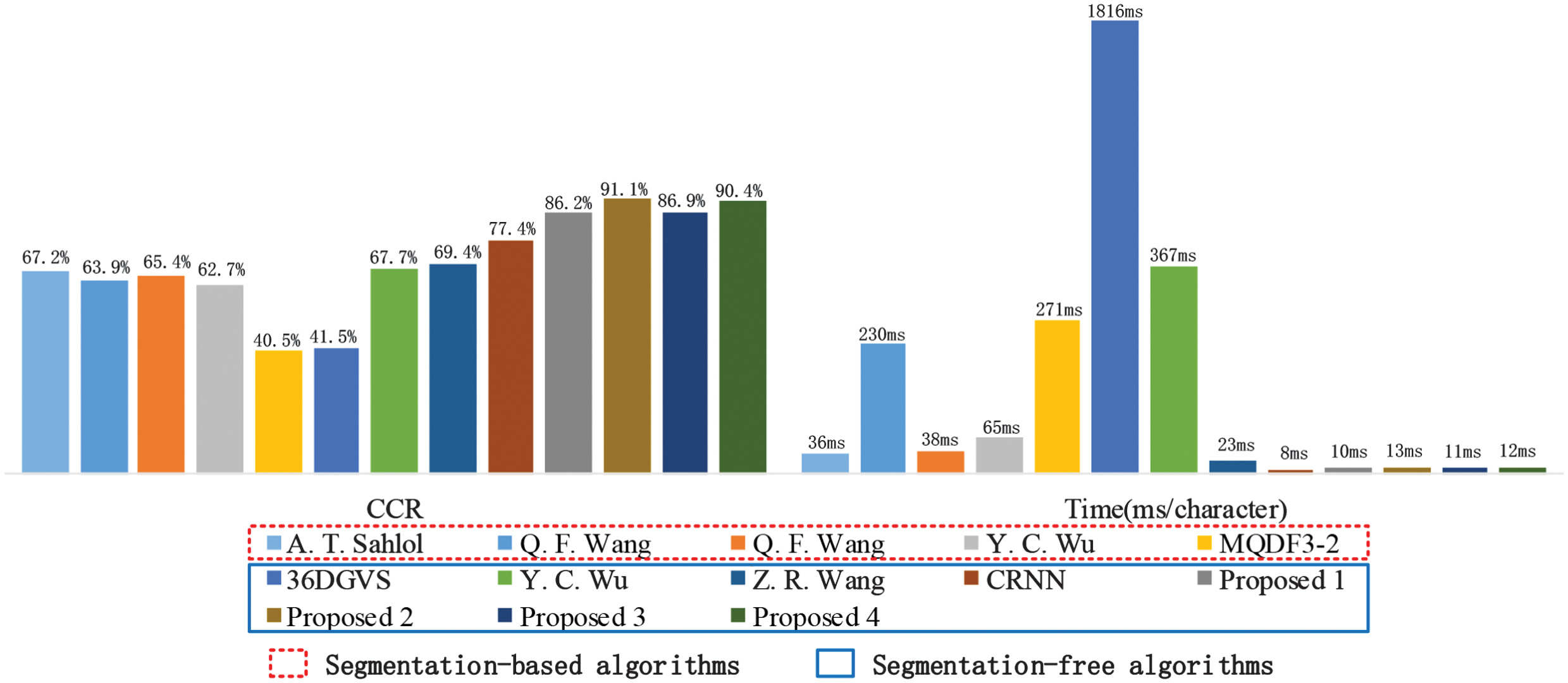Fig. 9. Comparison of testing accuracy. Histograms of average testing CCR and average testing time cost.

Table V. Comparisons with state-of-the-arts

Algorithms		IAM (%)	CASIA-HWDB (%)	HIT-MW (%)	DigitalPeter (%)	Rodrigo (%)	KHATT (%)	Model size (M)	Testing time (ms/character)
Segmentation-based algorithms	A. T. Sahlol [1]	57.23	93.72	92.39	52.31	53.55	54.25	—	36.2
	Q. F. Wang [10]	58.23	92.72	91.39	54.31	56.55	30.25	—	230
	Q. F. Wang [11]	53.65	92.19	86.56	56.98	59.54	43.56	—	38
	Y. C. Wu [13]	57.22	91.80	78.68	53.67	61.23	33.66	—	65
	MQDF3-2 [14]	37.89	38.59	35.49	55.68	45.25	30.15	—	271.4
Segmentation-free algorithms	36DGVS [14]	45.67	47.67	44.33	41.26	36.63	33.67	30.96	1816.2
	Y. C. Wu [17]	66.53	95.04	92.33	58.23	60.23	33.89	21.7	367
	Z. R. Wang [18]	67.53	95.93	93.12	59.64	60.03	40.12	107	23
	CRNN [19]	81.89	92.95	64.35	77.68	97.25	50.34	18.8	8
	Proposal 1	96.14	97.91	77.79	88.21	99.31	58.02	47.6	10.2
	Proposal 2	96.69	98.92	98.03	97.22	99.36	56.55	161	13.1
	Proposal 3	92.55	96.25	97.59	81.34	99.34	54.13	47.6	10.8
	Proposal 4	96.35	98.86	98.60	95.35	99.42	53.85	161	11.6

On the side of efficiency, the 36DGVS algorithm has the worst performance with a testing time cost of 1.81612 s per character and a mode size of 30.96 M. From Fig. 9, Proposal 2 and Proposal 4 occupy 161 M and 46.7 M more spaces than Proposed 1 and Proposal 2, respectively, due to the complexity in BDLSTM layers. However, it makes no significant difference in testing time. Proposal 1, 2, 3, and 4 algorithms take 10.2 ms, 13.1 ms, 10.8 ms, and 11.6 ms for one letter recognizing on CPU, respectively. Thus, Proposal 2 and Proposal 4 perform better in efficiency than the others except for the longer training time cost.

Overall, Proposal 2 and Proposal 4 prove useful in the task of sequence labeling with good accuracy and efficiency.

V.CONCLUSION

A segmentation-free handwritten text recognition algorithm based on deep networks is proposed to tackle the challenges of sequence labeling for handwritten manuscripts with interleaving and touching in this paper. The proposed framework consisted of preprocessing, CNNs, BDLSTM, and CTC loss layers. And six representative handwritten databases of different languages, including English, Chinese, Russian, Spanish, and Arabic, are used for comparison experiments on a group of typical segmentation-based and segmentation-free algorithms. The proposed networks were proven to be useful in the task of sequence labeling, where Arabic with several variant shapes need improved algorithm for better recognition results in the future works.

Segmentation-Free Recognition Algorithm Based on Deep Learning for Handwritten Text Image