JAIT

I.INTRODUCTION

Aggregation operators are a useful tool to convert all individual input data into single one and have a great importance in decision-making (DM), pattern recognition, medical diagnosis, and data mining, etc. In the past, decisions were made on the bases of crisp numbers, but that approach is less applicable in making the suitable decisions. To reduce such limitations, the concept of fuzzy set (FS) was initially introduced by Zadeh [1] in 1965 by consisting of only membership degree (MD) belonging to [0,1]. FS is a basic apparatus for handling the uncertain and enigmatic problems. Considerable developments of FS had been established such as interval-valued FS (IVFS) [2] in which MD is equal to interval value belonging to [0,1]. The idea of FSs was further generalized into an intuitionistic FS (IFS) by Atanassov [3] in which MD “ $μ \in [0, 1]$ ” as well as nonmembership degree (NMD) “ $ϑ \in [0, 1]$ ,” such that $0 \leq μ + ϑ \leq 1$ . Under such environment, some intuitionistic fuzzy (IF) weighted averaging (WA), IF ordered WA, and IF hybrid aggregation operators were defined by Xu [4]. The idea of IFS was further generalized into interval-valued IFS (IVIFS) by Atanassov [5]. Wang et al. [6] proposed WA and geometric aggregation operators. However, under some circumstances, when decision-makers evaluate the given object and provide “0.4” as an MD and “0.7” as an NMD, then it is clearly seen that IFS cannot be described effectively for handling such type of problems, because $0.4 + 0.7 > 1$ . To address it, a concept of Pythagorean FS (PFS) as an extension of IFS was established by Yager [7]. It is a broader concept in which MD “ $μ$ ” and NMD “ $ϑ$ ” must justify the situation $0 \leq μ^{2} + ϑ^{2} \leq 1$ . Furthermore, Pythagorean fuzzy (PF) power aggregation operators and PF Einstein prioritized aggregation operators for Pythagorean fuzzy numbers (PFNs) are discussed in [8] and [9], respectively. The concept of PFS was further generalized into interval-valued PFS (IVPFS) and some fundamental properties of IVPF aggregation operators were discussed by Peng and Yang [10] and Garg [11]. In addition, some averaging and geometric operators were discussed by Peng and Yang [10]. Furthermore, the q-rung orthopair fuzzy set (q-ROFS) proposed by Yager [12] can generalize IFS and PFS. In q-ROFS, MD “ $μ$ ” and NMD “ $ϑ$ ” must assure the condition $0 \leq μ^{q} + ϑ^{q} \leq 1$ for $q \geq 1$ . Some other views on q-ROFS are given in [13]. To address the q-ROFS in solving the DM problems, we refer to read [14 –16]. Ju et al. [17] established the idea of interval-valued q-ROFS (IVq-ROFS) and presented some averaging and geometric operators. Gao et al. [18] presented the IVq-ROF Archimedean Muirhead mean (MM) operators.

All the above studies are considered either the interval data or crisp data. Apart from it, the idea of cubic set (CS) was established by Jun et al. [19] using the combination of IVFS and FS and defined some basic operations on CSs. Fahmi et al. [20] introduced some cubic fuzzy Einstein aggregation operators and also discussed its applications to the judgment process. Also, the trapezoidal cubic fuzzy number Einstein hybrid WA operators are discussed in [21]. The idea of cubic hesitant fuzzy sets (CHFSs) was established by Mahmood et al. [22], and their aggregation operators are also defined. Furthermore, the idea of cubic intuitionistic fuzzy set (CIFS) as an extension of CS was established by Kaur and Garg [23], and some CIF aggregation operators are discussed in [24]. Abbas et al. [25] introduced the concept of cubic PF set (CPFS), and some cubic PF WA and cubic PF weighted geometric (WG) aggregation operators were defined by them. Wang et al. [26] introduced the concept of cubic q-ROFS (Cq-ROFS) and proposed power MM operator based on cubic q-rung orthopair fuzzy numbers (Cq-ROFNs), which can generalize both CIFS and CPFS.

From the above study, we have analyzed that there are many ideas over the generalization of FSs, which can be divided into two branches. One is based on quantitative FSs and the other on qualitative FSs that are usually denoted by linguistic variables. FS, IVFS, IFS, and IVIFS can only handle the vague information that is defined in quantitative regard. However, as the passage of the time, many DM problems present qualitative aspects of imprecise data. For example, if we assess the level of intelligence of a person, we usually utilize the linguistic term set (LTS) as $S = {very low, low, medium, high, very high}$ to describe it. To reduce this study deficiency and express the opinion in natural language, the concept of linguistic variable was established by Zadeh [27], [28]. Wang and Li [29] established the concept of IF linguistic set (IFLS) based on IFS and LVs, which present the MD and NMD of intuitionistic fuzzy numbers (IFNs) by linguistic variables (LVs). IFL operators were proposed by Liu et al. [30] to handle multiattribute group decision making (MAGDM) problems. Using the concept of linguistic variable and interval-valued fuzzy numbers (IVFNs), Xian et al. [31] developed the concept of IVIF linguistic set (IVIFLS) and proposed technique for order preference by similarity to the ideal solution (TOPSIS) method and operators based on IVIFLS. Peng and Yang [32] extended the concept of IFLS to PF linguistic set (PFLS) and established WA and WG operators based on Pythagorean fuzzy linguistic numbers (PFLNs). Also, Pythagorean Maclaurin symmetric mean aggregation operator was proposed by Teng et al. [33]. PFLS can express the vague information more precisely than that of IFLS. The idea of PFLS was further generalized into interval-valued PFLS (IVPFLS) proposed by Du et al. [34], and further averaging operators based on IVPFLS were established by them. Inspired by the concept of IFLS and PFLS, the concept of q-ROF linguistic set (q-ROFLS) was developed by Wang et al. [35], and some aggregation operators based on q-ROFLS were developed by them. Moreover, interval-valued q-rung orthopair 2-tuple linguistic aggregation operators were established by Wang et al. [36].

Because Cq-ROFS is more general than CIFSs and CPFSs in describing information, linguistic variables are the qualitative aspect of fuzzy information to deal with multiattribute decision-making (MADM), so from the aforementioned study, it is required to handle the fuzzy information defined in qualitative aspect. Therefore, to overcome the limitation of CIFS and CPFS, in this paper, we first establish the basic concept of cubic q-rung orthopair fuzzy linguistic set (Cq-ROFLS). MM operator can establish the association between all input arguments. Therefore, the goal of this paper is to establish some methods for MADM problems for Cq-ROFL information based on some new Cq-ROFL MM (Cq-ROFLMM) operators by combining the MM operator and Cq-ROFL information. Keeping the advantages of MM operators and by the concept of Cq-ROFLS, we propose a new cubic q-rung orthopair fuzzy linguistic Muirhead mean- (MM), weighted MM-, dual MM-based aggregation operators, denoted by Cq-ROFLMM, weighted Cq-ROFLMM (Cq-ROFLWMM), Cq-ROFLDMM, and Cq-ROFLDWMM operators, respectively. Moreover, the properties of these operators are discussed. DM approach has been proposed based on established work for the selection of best solution. A numerical example is explored to explain the given approach.

The rest of this paper is summarized as follows: In Section II, we briefly review the basic definition related to q-ROFSs and others. In Section III, we present the concept of Cq-ROFLS and study its basic operations. In Section IV, we establish MM, dual MM operators and their weighted forms. In Section V, an algorithm for solving the MADM problem based on the proposed MM operators with Cq-ROFLS information is described and illustrated with a case study. The efficiency of the proposed algorithm is compared with the existing studies in detail. Finally, Section VI concludes the remarks.

II.PRELIMINARIES

In this section, we briefly overview some definitions over the nonempty universal set.

Definition 1:[12] A q-ROFS on $X$ is given as $Ѧ = {< ϰ, M_{Ѧ} (ϰ), N_{Ѧ} (ϰ) > | ϰ \in X}$ , where $M_{Ѧ} (ϰ)$ and $N_{Ѧ} (ϰ)$ are MD and NMD, respectively, having extra condition that $0 \leq {(M_{Ѧ} (ϰ))}^{q} + {(N_{Ѧ} (ϰ))}^{q} \leq 1$ , where $q \geq 1$ . In general, $h_{Ѧ} (ϰ) = \sqrt[q]{1 - (M_{Ѧ} (ϰ))^{q} - (N_{Ѧ} (ϰ))^{q}}$ is the hesitancy degree of $ϰ$ to $Ѧ$ . For simplicity, $Ѧ = 〈 M_{Ѧ}, N_{Ѧ} 〉$ denotes the q-ROFN.

Definition 2:[17] An IVq-ROFS on $X$ is a set $Ѧ = {< ϰ, M_{Ѧ} (ϰ), N_{Ѧ} (ϰ) > | ϰ \in X}$ , where $0 \leq M_{Ѧ} (ϰ) \leq 1$ and $0 \leq N_{Ѧ} (ϰ) \leq 1$ are MD and NMD, respectively, $M_{Ѧ} (ϰ) = [M_{Ѧ}^{L} (ϰ), M_{Ѧ}^{U} (ϰ)]$ , $N_{Ѧ} (ϰ) = [N_{Ѧ}^{L} (ϰ), N_{Ѧ}^{U} (ϰ)]$ with the condition $0 \leq (M_{Ѧ}^{U} (ϰ))^{q} + (N_{Ѧ}^{U} (ϰ))^{q} \leq 1$ , $\forall ϰ \in X$ , $q \geq 1$ . $h_{Ѧ} (ϰ) = [h_{Ѧ}^{L} (ϰ), h_{Ѧ}^{U} (ϰ)] = [\sqrt[q]{1 - ((M_{Ѧ}^{U} (ϰ))^{q} + (N_{Ѧ}^{U} (ϰ))^{q})}, \sqrt[q]{1 - ((M_{Ѧ}^{L} (ϰ))^{q} + (N_{Ѧ}^{L} (ϰ))^{q})}]$ is called refusal degree of $ϰ$ to $Ѧ$ .

Definition 3:[18] Let $β_{ɨ} (ɨ = 1, 2, \dots, ņ)$ be a family of positive real numbers, and $Ƀ = {β_{1}, β_{2}, \dots, β_{ņ}}$ and $p = (p_{1}, p_{2}, \dots, p_{ņ}) \in R^{ņ}$ be a parameter vector (PV), if

{M M}^{p} (β_{1}, β_{2}, \dots, β_{ņ}) = (\frac{1}{ņ!} (\sum_{θ \in s_{ņ}} (\prod_{ʝ = 1}^{ņ} β_{θ (ʝ)}^{p_{ʝ}})))^{\frac{1}{\sum_{ʝ = 1}^{ņ} p_{ʝ}}} .

(1)

Then,

{M M}^{p}

is called MM operator, which is simply denoted by MM, where

θ (ʝ) (ʝ = 1, 2, 3, \dots, ņ)

denotes any permutation of (

1, 2, 3, \dots, ņ

) and

s_{ņ}

denotes the family of all permutation

θ (ʝ) (ʝ = 1, 2, 3, \dots, ņ)

Definition 4:[26] A Cq-ROFS is stated as

C = {< ϰ, Ѧ (ϰ), λ (ϰ) >},

(2)

where

Ѧ (ϰ)

is an IVq-ROFS and

λ (ϰ)

is a q-ROFS. Here,

Ѧ (x) = {[ч^{L}, ч^{U}], [ѵ^{L}, ѵ^{U}]}

with

0 \leq ({ч^{U})}^{q} + {(ѵ^{U})}^{q} \leq 1

and

λ (ϰ) = (ч, ѵ)

with

0 \leq ч^{q} + ѵ^{q} \leq 1

. For simplicity, we denote this pair as

C = {< Ѧ, λ >}

, where

Ѧ = {[ч^{L}, ч^{U}], [ѵ^{L}, ѵ^{U}]}

and

λ = (ч, ѵ)

, and are called Cq-ROFN.

A Cq-ROFS “ $C$ ” defined in (2) is called internal Cq-ROFS, if $ч \in [ч^{L}, ч^{U}]$ and $ѵ \in [ѵ^{L}, ѵ^{U}]$ for all $ϰ \in X$ , otherwise called external Cq-ROFS.

Definition 5:[26] Let $C_{1} = (([ч_{1}^{L}, ч_{1}^{U}], [ѵ_{1}^{L}, ѵ_{1}^{U}]), (ч_{1}, ѵ_{1}))$ and $C_{2} = (([ч_{2}^{L}, ч_{2}^{U}], [ѵ_{2}^{L}, ѵ_{2}^{U}]), (ч_{2}, ѵ_{2}))$ be the two Cq-ROFNs and $K > 0$ , the operational laws are given as follows:

C_{1} \oplus C_{2} = ((\begin{matrix} [\begin{matrix} {({(ч_{1}^{L})}^{q} + {(ч_{2}^{L})}^{q} - {(ч_{1}^{L})}^{q} {(ч_{2}^{L})}^{q})}^{\frac{1}{q}}, \\ {({(ч_{1}^{U})}^{q} + {(ч_{2}^{U})}^{q} - {(ч_{1}^{U})}^{q} {(ч_{2}^{U})}^{q})}^{\frac{1}{q}} \end{matrix}], \\ [ѵ_{1}^{L} ѵ_{2}^{L}, ѵ_{1}^{U} ѵ_{2}^{U}] \end{matrix}), (\begin{matrix} {(ч_{1})}^{q} + {(ч_{2})}^{q} - {(ч_{1})}^{q} {(ч_{2})}^{q}, \\ ѵ_{1} ѵ_{2} \end{matrix})),

C_{1} \otimes C_{2} = ((\begin{matrix} [ч_{1}^{L} ч_{2}^{L}, ч_{1}^{U} ч_{2}^{U}], \\ [\begin{matrix} {({(ѵ_{1}^{L})}^{q} + {(ѵ_{2}^{L})}^{q} - {(ѵ_{1}^{L})}^{q} {(ѵ_{2}^{L})}^{q})}^{\frac{1}{q}}, \\ {({(ѵ_{1}^{U})}^{q} + {(ѵ_{2}^{U})}^{q} - {(ѵ_{1}^{U})}^{q} {(ѵ_{2}^{U})}^{q})}^{\frac{1}{q}} \end{matrix}] \end{matrix}), (\begin{matrix} ч_{1} ч_{2} \\ {(ѵ_{1})}^{q} + {(ѵ_{2})}^{q} - {(ѵ_{1})}^{q} {(ѵ_{2})}^{q} \end{matrix})),

K C_{1} = (([\begin{matrix} ({({1 - (1 - {ч_{1}^{L}}^{q})}^{K})}^{\frac{1}{q}}), \\ {({1 - (1 - {ч_{1}^{U}}^{q})}^{K})}^{\frac{1}{q}} \end{matrix}], [{ѵ_{1}^{L}}^{K}, {ѵ_{1}^{U}}^{K}]), (\begin{matrix} {(1 - ({(1 - ч_{1}^{q})}^{K}))}^{\frac{1}{q}}, \\ ѵ_{1}^{K} \end{matrix})),

C_{1}^{K} = (([{ч_{1}^{L}}^{K}, {ч_{1}^{U}}^{K}], [\begin{matrix} ({({1 - (1 - {ѵ_{1}^{L}}^{q})}^{K})}^{\frac{1}{q}}), \\ {({1 - (1 - {ѵ_{1}^{U}}^{q})}^{K})}^{\frac{1}{q}} \end{matrix}]), (\begin{matrix} ч_{1}^{K}, \\ {(1 - ({(1 - ѵ_{1}^{q})}^{K}))}^{\frac{1}{q}} \end{matrix})) .

III.CQ-ROFLS

In this section, we discuss the idea of Cq-ROFLS and its basic operations.

Let $L = {l_{0}, l_{1}, \dots, l_{f}}$ be a finite LTS with odd cardinality, where $l_{ɨ}$ represents the possible value for linguistic terms (LTs), $f + 1$ is the cardinality of $L$ . For example, $L = {l_{0} = extremely poor, l_{1} = very poor, l_{2} = poor, l_{3} = fair, l_{4} = good, l_{5} = very good, l_{6} = extremely good}$ . Clearly, the mid-linguistic expression shows an evaluation of “inattention,” and all remaining LTs are put proportionally around it.

Let $l_{ɨ}$ and $l_{ʝ}$ be any two LTs in LTS $L$ ; they have to satisfy the following conditions:

(1)if $ɨ > ʝ$ , then $l_{ɨ} > l_{ʝ}$ ,
(2)their exist a negative operator, $Neg (l_{ɨ}) = l_{ʝ}$ , such that $ʝ = f - ɨ$ ,
(3)if $l_{ɨ} > l_{ʝ}$ , then $\max (l_{ɨ}, l_{ʝ}) = l_{ɨ}$ and $\min (l_{ɨ}, l_{ʝ}) = l_{ʝ}$ .

The distinct LTS ‘ $L$ ’ can be extended to a continual LTS $\bar{L} = {l_{β} | β \in [0, f]}$ . If $l_{β} \in L$ , then $l_{β}$ is called the original LT, and if $l_{β} \notin L$ , then $l_{β}$ is called the virtual LT. Usually, the decisionmakers use original LT for the selection of best alternative, and virtual terms can appear only in calculations.

Definition 6:Let $X = {ϰ_{1}, ϰ_{2}, \dots, ϰ_{ņ}}$ be a universal set and $\bar{L} = {l_{0}, l_{1}, l_{2}, \dots, l_{f}}$ be a continual LTS, a Cq-ROFLS $C$ is given by

C = {< ϰ, s_{ϕ} (ϰ), (Ѧ (ϰ), λ (ϰ)) > | ϰ \in X},

(3)

where

s_{ϕ} (ϰ) \in \bar{L}

ч : X \to [0, 1]

denotes the MD,

ѵ : X \to [0, 1]

denotes the NMD of the element

ϰ \in X

to the LT

s_{ϕ} (ϰ)

Ѧ (ϰ)

is an IVq-ROFS, and

λ (ϰ)

is a q-ROFS. Here,

Ѧ (x) = {[ч^{L}, ч^{U}], [ѵ^{L}, ѵ^{U}]}

with

0 \leq ({ч^{U})}^{q} + {(ѵ^{U})}^{q} \leq 1

and

λ (ϰ) = (ч, ѵ)

with

0 \leq ч^{q} + ѵ^{q} \leq 1

. For simplicity, we denote cubic q-rung orthopair fuzzy linguistic numbers (Cq-ROFLNs) by

β = {< s_{θ (β)}, (Ѧ (β), λ (β)) >}

Ѧ = {[ч^{L}, ч^{U}], [ѵ^{L}, ѵ^{U}]}

, and

λ = (ч, ѵ)

and are called Cq-ROFN.

Definition 7:Let $β_{1} = (s_{ϕ_{1}}, (([ч_{1}^{L}, ч_{1}^{U}], [ѵ_{1}^{L}, ѵ_{1}^{U}]), (ч_{1}, ѵ_{1})))$ and $β_{2} = (s_{ϕ_{2}}, (([ч_{2}^{L}, ч_{2}^{U}], [ѵ_{2}^{L}, ѵ_{2}^{U}]), (ч_{2}, ѵ_{2})))$ be any two Cq-ROFLNs and $K > 0$ , then

β_{1} \oplus β_{2} = {s_{1 + ϕ_{2}}, ([\begin{matrix} {({ч_{1}^{L}}^{q} + {ч_{2}^{L}}^{q} - {ч_{1}^{L}}^{q} {ч_{2}^{L}}^{q})}^{\frac{1}{q}}, \\ {({ч_{1}^{U}}^{q} + {ч_{2}^{U}}^{q} - {ч_{1}^{U}}^{q} {ч_{2}^{U}}^{q})}^{\frac{1}{q}} \end{matrix}], [\begin{matrix} {ѵ_{1}^{L}}^{q} {ѵ_{2}^{L}}^{q}, \\ {ѵ_{1}^{U}}^{q} {ѵ_{2}^{U}}^{q} \end{matrix}]), (\begin{matrix} {(ч_{1}^{q} + ч_{2}^{q} - ч_{1}^{q} ч_{2}^{q})}^{\frac{1}{q}}, \\ ѵ_{1} ѵ_{2} \end{matrix})},

β_{1} \otimes β_{2} = {s_{ϕ_{1} \times ϕ_{2}}, ([ч_{1}^{L} ч_{2}^{L}, ч_{1}^{U} ч_{2}^{U}], [\begin{matrix} {({ѵ_{1}^{L}}^{q} + {ѵ_{2}^{L}}^{q} - {ѵ_{1}^{L}}^{q} {ѵ_{2}^{L}}^{q})}^{\frac{1}{q}}, \\ {({ѵ_{1}^{U}}^{q} + {ѵ_{2}^{U}}^{q} - {ѵ_{1}^{U}}^{q} {ѵ_{2}^{U}}^{q})}^{1 / q} \end{matrix}]), (\begin{matrix} ч_{1} ч_{2}, \\ ({(ѵ_{1}^{q} + ѵ_{2}^{q} - ѵ_{1}^{q} ѵ_{2}^{q})}^{1 / q}) \end{matrix}),},

K β_{1} = {s_{K \times ϕ_{2}}, ([\begin{matrix} ({({1 - (1 - {ч_{1}^{L}}^{q})}^{K})}^{\frac{1}{q}}), \\ {({1 - (1 - {ч_{1}^{U}}^{q})}^{K})}^{\frac{1}{q}} \end{matrix}], [{ѵ_{1}^{L}}^{K}, {ѵ_{1}^{U}}^{K}]), (\begin{matrix} {(1 - ({(1 - ч_{1}^{q})}^{K}))}^{\frac{1}{q}}, \\ ѵ_{1}^{K} \end{matrix})},

β_{1}^{K} = {{s_{ϕ_{1}}}^{K}, ([{ч_{1}^{L}}^{K}, {ч_{1}^{U}}^{K}], [\begin{matrix} ({({1 - (1 - {ѵ_{1}^{L}}^{q})}^{K})}^{\frac{1}{q}}), \\ {({1 - (1 - {ѵ_{1}^{U}}^{q})}^{K})}^{\frac{1}{q}} \end{matrix}]), (\begin{matrix} ч_{1}^{K}, \\ {(1 - ({(1 - ѵ_{1}^{q})}^{K}))}^{\frac{1}{q}} \end{matrix})} .

Definition 8:Let $β_{1} = (s_{ϕ_{1}}, (([ч_{1}^{L}, ч_{1}^{U}], [ѵ_{1}^{L}, ѵ_{1}^{U}]), (ч, ѵ)))$ be a Cq-ROFLN, then score and accuracy functions for $β_{1}$ are defined as

S c (β_{1}) = \frac{1}{2} [\frac{1}{4} [(1 + {{(ч}_{1}^{L})}^{q} - {{(ѵ}_{1}^{L})}^{q}) + (1 + {{(ч}_{1}^{U})}^{q} - {{(ѵ}_{1}^{U})}^{q})] + (ч_{1}^{q} - ѵ_{1}^{q})] \times ϕ_{1},

(4)

and

H (β_{1}) = \frac{1}{2} [\frac{1}{2} [({{(ч}_{1}^{L})}^{q} + {{(ч}_{1}^{U})}^{q}) + ({{(ѵ}_{1}^{L})}^{q} + {{(ѵ}_{1}^{U})}^{q})] + (ч_{1}^{q} + ѵ_{1}^{q})] \times ϕ_{1} .

(5)

Furthermore, based on these functions, the comparison rule for two Cq-ROFLNs is defined as follows:

(1)If $S c (β_{1}) < S c (β_{2})$ , then $β_{1}$ is preferable over $β_{2}$ and is denoted by $β_{1} ≺ β_{2}$ .
(2)If $S c (β_{1}) = S c (β_{2})$ and $H (β_{1}) < H (β_{2})$ , then $β_{1} ≺ β_{2}$ .

IV.CQ-ROFLMM OPERATOR

Because the traditional $M M$ operator deals with crisp numbers and Cq-ROFNs easily describe the fuzzy data, it is required to expand the traditional MM operator to Cq-ROFLMM operator. So here, we will establish Cq-ROFLMM operator and its weighted form. Moreover, their properties are also discussed.

Definition 9:Let $β_{ɨ} = (s_{ϕ_{ɨ}}, (([ч_{ɨ}^{L}, ч_{ɨ}^{U}], [ѵ_{ɨ}^{L}, ѵ_{ɨ}^{U}]), (ч_{ɨ}, ѵ_{ɨ})))$ be a collection of Cq-ROFLNs, and $Ƀ = {β_{1}, β_{2}, \dots, β_{ņ}}$ and $p = (p_{1}, p_{2}, \dots, p_{ņ}) \in R^{ņ}$ denote a PV, a Cq-ROFLMM operator is a mapping

Cq - {ROFLMM}^{p} (β_{1}, β_{2}, \dots ., β_{ņ}) = {(\frac{1}{ņ!} (\oplus_{ϑ \in s_{ņ}} (\otimes_{ʝ = 1}^{ņ} β_{ϑ (ʝ)}^{p_{ʝ}})))}^{\frac{1}{\sum_{ʝ = 1}^{ņ} p_{ʝ}}},

(6)

where

ϑ (ʝ) (ʝ = 1, 2, 3, \dots, ņ)

denotes permutation of (

1, 2, 3, \dots, ņ

) and

s_{ņ}

denotes family of all permutation of

ϑ (ʝ) (ʝ = 1, 2, 3, \dots, ņ)

Theorem 1:Suppose $β_{ɨ} = (s_{ϕ_{ɨ}}, (([ч_{ɨ}^{L}, ч_{ɨ}^{U}], [ѵ_{ɨ}^{L}, ѵ_{ɨ}^{U}]), (ч_{ɨ}, ѵ_{ɨ})))$ be a collection of Cq-ROFLNs and $p = (p_{1}, p_{2}, \dots, p_{ņ}) \in R^{ņ}$ denote a PV, then $Cq - {ROFLMM}^{p} (β_{1}, β_{2}, \dots, β_{n})$ is also a Cq-ROFLN and

Cq - {ROFLMM}^{p} (β_{1}, β_{2}, \dots, β_{n}) = (\begin{matrix} s_{{(\frac{1}{ņ!} (\sum_{ϑ \in s_{ņ}} (\prod_{ʝ = 1}^{ņ} ϕ_{ϑ (ʝ)}^{p_{ʝ}})))}^{\frac{1}{\sum_{ʝ = 1}^{ņ} p_{ʝ}}}}, (\begin{matrix} [\begin{matrix} {(\sqrt[q]{1 - {(\prod_{ϑ \in s_{ņ}} (1 - {(\prod_{ʝ = 1}^{ņ} {ч^{L}}_{ϑ (ʝ)}^{p_{ʝ}})}^{q}))}^{\frac{1}{ņ!}}})}^{\frac{1}{\sum_{ʝ = 1}^{ņ} p_{ʝ}}}, \\ {(\sqrt[q]{1 - {(\prod_{ϑ \in s_{ņ}} (1 - {(\prod_{ʝ = 1}^{ņ} {ч^{U}}_{ϑ (ʝ)}^{p_{ʝ}})}^{q}))}^{\frac{1}{ņ!}}})}^{\frac{1}{\sum_{ʝ = 1}^{ņ} p_{ʝ}}} \end{matrix}], \\ [\begin{matrix} \sqrt[q]{1 - {(1 - {(\prod_{ϑ \in s_{ņ}} (1 - \prod_{ʝ = 1}^{ņ} {(1 - {ѵ^{L}}_{ϑ (ʝ)}^{q})}^{p_{ʝ}}))}^{\frac{1}{ņ!}})}^{\frac{1}{\sum_{ʝ = 1}^{ņ} p_{ʝ}}}}, \\ \sqrt[q]{1 - {(1 - {(\prod_{ϑ \in s_{ņ}} (1 - \prod_{ʝ = 1}^{ņ} {(1 - {ѵ^{U}}_{ϑ (ʝ)}^{q})}^{p_{ʝ}}))}^{\frac{1}{ņ!}})}^{\frac{1}{\sum_{ʝ = 1}^{ņ} p_{ʝ}}}} \end{matrix}] \end{matrix}), \\ (\begin{matrix} {(\sqrt[q]{1 - {(\prod_{ϑ \in s_{ņ}} (1 - {(\prod_{ʝ = 1}^{ņ} ч_{ϑ (ʝ)}^{p_{ʝ}})}^{q}))}^{\frac{1}{ņ!}}})}^{\frac{1}{\sum_{ʝ = 1}^{ņ} p_{ʝ}}}, \\ \sqrt[q]{1 - {(1 - {(\prod_{ϑ \in s_{ņ}} (1 - \prod_{ʝ = 1}^{ņ} {(1 - ѵ_{ϑ (ʝ)}^{q})}^{p_{ʝ}}))}^{\frac{1}{ņ!}})}^{\frac{1}{\sum_{ʝ = 1}^{ņ} p_{ʝ}}}} \end{matrix}) \end{matrix}) .

(7)

Proof:Based on the operations of Cq-ROFLNs defined in Definition 8 and (6), we can easily deduce the required result.

It has been observed that the proposed Cq-ROFLMM operator satisfies certain properties which are stated below.

Property 1:(Idempotency) Let $β_{ɨ}$ be a collection of Cq-ROFLNs and $p = (p_{1}, p_{2}, \dots, p_{ņ}) \in R^{ņ}$ be a PV, if all $β_{ɨ} = β$ , then

Cq - {ROFLMM}^{p} (β_{1}, β_{2}, \dots ., β_{ņ}) = β .

Proof:Since $β_{ɨ} = β$ , so from (6), we have

Cq - {ROFLMM}^{p} (β_{1}, β_{2}, \dots ., β_{ņ}) = (\frac{1}{ņ!} (\oplus_{ϑ \in s_{ņ}} (\otimes_{ʝ = 1}^{ņ} β^{p_{j}})))^{\frac{1}{\sum_{ʝ = 1}^{ņ} p_{ʝ}}} = (\frac{1}{ņ!} (\oplus_{ϑ \in s_{ņ}} (β^{\sum_{j = 1} p_{j}})))^{\frac{1}{\sum_{ʝ = 1}^{ņ} p_{ʝ}}} = β .

Property 2:(Monotonicity) Let $β_{ɨ} = (s_{ϕ_{ɨ}}, (([ч_{ɨ}^{L}, ч_{ɨ}^{U}], [ѵ_{ɨ}^{L}, ѵ_{ɨ}^{U}]), (ч_{ɨ}, ѵ_{ɨ}))) (ɨ = 1, 2, 3, \dots, ņ)$ and ${β_{ɨ}}^{'} = (s_{{ϕ_{ɨ}}^{'}}, (([{ч_{ɨ}}^{'}^{L}, ч_{ɨ}^{'^{U}}], [ѵ_{ɨ}^{'^{L}}, ѵ_{ɨ}^{'^{U}}]), ({ч_{ɨ}}^{'}, {ѵ_{ɨ}}^{'})))$ be two collections of Cq-ROFLNs and $p = (p_{1}, p_{2}, \dots, p_{ņ}) \in R^{ņ}$ be a PV, if $s_{ϕ_{ɨ}} \leq s_{{ϕ_{ɨ}}^{'}}, [ч_{ɨ}^{L}, ч_{ɨ}^{U}] \leq [{ч_{ɨ}}^{'}^{L}, ч_{ɨ}^{'^{U}}], [ѵ_{ɨ}^{L}, ѵ_{ɨ}^{U}] \geq [ѵ_{ɨ}^{'^{L}}, ѵ_{ɨ}^{'^{U}}]$ and $ч_{ɨ} \leq {ч^{'}}_{ɨ}, ѵ_{ɨ} \geq {ѵ^{'}}_{ɨ}$ , then

Cq - {ROFLMM 1}^{p} (β_{1}, β_{2}, \dots, β_{ņ}) \leq Cq - {ROFLMM}^{p} ({β_{1}}^{'}, {β_{2}}^{'}, \dots, {β_{ņ}}^{'}) .

Proof:It can be easily derived follows from (7). Hence, we omit here.

Property 3:(Boundedness) For a collection of Cq-ROFLNs $β_{ɨ}$ , let lower and upper bounds of $β^{'} s$ are $β^{-}$ and $β^{+}$ , then

β^{-} \leq Cq - {ROFLMM}^{p} (β_{1}, β_{2}, \dots, β_{ņ}) \leq β^{+} .

Proof:Follow from Properties 1 and 2.

Now, we examine some particular cases of Cq-ROFLMM operator according to the PV.

For a collection of Cq-ROFLNs, $β_{ɨ}$ and $p = (p_{1}, p_{2}, \dots, p_{ņ}) \in R^{ņ}$ be a PV.

(a)If $p = (1, 0, 0, 0, \dots, 0)$ , Cq-ROFLMM operator reduces to the Cq-ROFL arithmetic averaging operator, that is,
$Cq - {ROFLMM}^{(1, 0, 0, 0, \dots, 0)} (β_{1}, β_{2}, \dots, β_{n}) = (\begin{matrix} s_{\frac{\sum_{ʝ = 1}^{ņ} ϕ_{ɨ}}{ņ}}, ([\sqrt[q]{1 - \prod_{ʝ = 1}^{ņ} (1 - {ч^{L}}_{ʝ}^{q})^{\frac{1}{ņ}}}, \sqrt[q]{1 - \prod_{ʝ = 1}^{ņ} (1 - {ч^{U}}_{ʝ}^{q})^{\frac{1}{ņ}}}], [\prod_{ʝ = 1}^{ņ} {ѵ^{L}}_{ʝ}^{\frac{1}{ņ}}, \prod_{ʝ = 1}^{ņ} {ѵ^{U}}_{ʝ}^{\frac{1}{ņ}}]), \\ ([\sqrt[q]{1 - \prod_{ʝ = 1}^{ņ} {(1 - ч_{ʝ}^{q})}^{\frac{1}{ņ}}}, \prod_{ʝ = 1}^{ņ} ѵ_{ʝ}^{\frac{1}{ņ}}]) \end{matrix}) .$ (8)
(b)If $p = (τ, 0, 0, 0, \dots, 0)$ , Cq-ROFLMM operator reduces to
$Cq - {ROFLMM}^{(τ, 0, 0, 0, \dots, 0)} (β_{1}, β_{2}, \dots, β_{n}) = (\begin{matrix} s_{{(\frac{\sum_{ʝ = 1}^{ņ} {ϕ_{ɨ}}^{τ}}{ņ})}^{\frac{1}{τ}}}, (\begin{matrix} [\begin{matrix} {(\sqrt[q]{1 - \prod_{ʝ = 1}^{ņ} {(1 - {ч^{L}}_{ʝ}^{q τ})}^{\frac{1}{ņ}}})}^{\frac{1}{τ}}, \\ {(\sqrt[q]{1 - \prod_{ʝ = 1}^{ņ} {(1 - {ч^{U}}_{ʝ}^{q τ})}^{\frac{1}{ņ}}})}^{\frac{1}{τ}} \end{matrix}], \end{matrix} [\begin{matrix} \sqrt[q]{1 - {(1 - \prod_{ʝ = 1}^{ņ} {(1 - {(1 - {ѵ^{L}}_{ʝ}^{q})}^{τ})}^{\frac{1}{ņ}})}^{\frac{1}{τ}}}, \\ \sqrt[q]{1 - {(1 - \prod_{ʝ = 1}^{ņ} {(1 - {(1 - {ѵ^{U}}_{ʝ}^{q})}^{τ})}^{\frac{1}{ņ}})}^{\frac{1}{τ}}} \end{matrix}]), \\ ([\begin{matrix} \sqrt[q]{1 - \prod_{ʝ = 1}^{ņ} {(1 - ч_{ʝ}^{q})}^{\frac{1}{ņ}}}, \\ \sqrt[q]{1 - {(1 - \prod_{ʝ = 1}^{ņ} {(1 - {(1 - ѵ_{ʝ}^{q})}^{τ})}^{\frac{1}{ņ}})}^{\frac{1}{τ}}} \end{matrix}]) \end{matrix}) .$ (9)
(c)If $p = (\underset{k}{\underset{︸}{1, 1, 1, 1, \dots, 1}}, \underset{ņ - k}{\underset{︸}{0, 0, 0, \dots, 0}})$ , Cq-ROFLMM operator converts into Cq-ROFL Maclaurin symmetric mean operator, that is,
${Cq - ROFLMM}^{(\underset{k}{\underset{︸}{1, 1, 1, 1, \dots, 1}}, \underset{ņ - k}{\underset{︸}{0, 0, 0, \dots, 0}})} (β_{1}, β_{2}, \dots, β_{n}) = (\begin{matrix} s_{{(\frac{1}{{D_{ņ}}^{k}} (\sum_{1 \leq ɨ_{1} \leq \dots . \leq ɨ_{k \leq} 1} (\prod_{ʝ = 1}^{ņ} ϕ_{ɨ_{ʝ}})))}^{\frac{1}{k}}}, (\begin{matrix} [\begin{matrix} \sqrt[q]{{(1 - \prod_{1 \leq ɨ_{1} \leq \dots . \leq ɨ_{k \leq} ņ} {(1 - \prod_{ʝ = 1}^{ņ} {ч^{L}}_{ɨ_{ʝ}}^{q})}^{\frac{1}{D_{ņ}^{k}}})}^{\frac{1}{k}}}, \\ \sqrt[q]{{(1 - \prod_{1 \leq ɨ_{1} \leq \dots . \leq ɨ_{k \leq} ņ} {(1 - \prod_{ʝ = 1}^{ņ} {ч^{U}}_{ɨ_{ʝ}}^{q})}^{\frac{1}{D_{ņ}^{k}}})}^{\frac{1}{k}}} \end{matrix}], \end{matrix} [\begin{matrix} \sqrt[q]{1 - {(1 - (\prod_{1 \leq ɨ_{1} \leq \dots . \leq ɨ_{k \leq} ņ} {(1 - \prod_{ʝ = 1}^{ņ} (1 - {ѵ^{L}}_{ɨ_{ʝ}}^{q}))}^{\frac{1}{D_{ņ}^{k}}}))}^{\frac{1}{k}}}, \\ \sqrt[q]{1 - {(1 - (\prod_{1 \leq ɨ_{1} \leq \dots . \leq ɨ_{k \leq} ņ} {(1 - \prod_{ʝ = 1}^{ņ} (1 - {ѵ^{U}}_{ɨ_{ʝ}}^{q}))}^{\frac{1}{D_{ņ}^{k}}}))}^{\frac{1}{k}}} \end{matrix}]), \\ (\begin{matrix} \sqrt[q]{{(1 - \prod_{1 \leq ɨ_{1} \leq \dots . \leq ɨ_{k \leq} ņ} {(1 - \prod_{ʝ = 1}^{ņ} ч_{ɨ_{ʝ}}^{q})}^{\frac{1}{D_{ņ}^{k}}})}^{\frac{1}{k}}}, \\ \sqrt[q]{1 - {(1 - (\prod_{1 \leq ɨ_{1} \leq \dots . \leq ɨ_{k \leq} ņ} {(1 - \prod_{ʝ = 1}^{ņ} (1 - ѵ_{ɨ_{ʝ}}^{q}))}^{\frac{1}{D_{ņ}^{k}}}))}^{\frac{1}{k}}} \end{matrix}) \end{matrix}) .$ (10)
(d)If $p = (1, 1, 1, 1, \dots, 1)$ , Cq-ROFLMM operator converts into the Cq-ROFL geometric averaging operator, that is,
${Cq - ROFLMM}^{(1, 1, 1, 1, \dots, 1)} (β_{1}, β_{2}, \dots, β_{n}) = (\begin{matrix} s_{\prod_{ʝ = 1}^{ņ} ϕ_{ʝ}^{\frac{1}{ņ}}}, ([{(\prod_{ʝ = 1}^{ņ} ч_{ʝ}^{L})}^{\frac{1}{ņ}}, {(\prod_{ʝ = 1}^{ņ} ч_{ʝ}^{U})}^{\frac{1}{ņ}}], [\begin{matrix} \sqrt[q]{1 - {(\prod_{ʝ = 1}^{ņ} (1 - {ѵ^{L}}_{ʝ}^{q}))}^{\frac{1}{ņ}}}, \\ \sqrt[q]{1 - {(\prod_{ʝ = 1}^{ņ} (1 - ѵ_{ʝ}^{q}))}^{\frac{1}{ņ}}} \end{matrix}]), \\ ([{(\prod_{ʝ = 1}^{ņ} ч_{ʝ})}^{\frac{1}{ņ}}, \sqrt[q]{1 - {(\prod_{ʝ = 1}^{ņ} (1 - ѵ_{ʝ}^{q}))}^{\frac{1}{ņ}}}]) \end{matrix}) .$ (11)
(e)If $p = (\frac{1}{ņ}, \frac{1}{ņ}, \frac{1}{ņ}, \frac{1}{ņ}, \dots, \frac{1}{ņ})$ , the Cq-ROFLMM operator becomes
${Cq - ROFLMM}^{(\frac{1}{ņ}, \frac{1}{ņ}, \dots ., \frac{1}{ņ})} (β_{1}, β_{2}, \dots, β_{n}) = (\begin{matrix} s_{\prod_{ʝ = 1}^{ņ} ϕ_{ʝ}^{\frac{1}{ņ}}}, ([{(\prod_{ʝ = 1}^{ņ} ч_{ʝ}^{L})}^{\frac{1}{ņ}}, {(\prod_{ʝ = 1}^{ņ} ч_{ʝ}^{U})}^{\frac{1}{ņ}}], [\begin{matrix} \sqrt[q]{1 - {(\prod_{ʝ = 1}^{ņ} (1 - {ѵ^{L}}_{ʝ}^{q}))}^{\frac{1}{ņ}}}, \\ \sqrt[q]{1 - {(\prod_{ʝ = 1}^{ņ} (1 - {ѵ^{U}}_{ʝ}^{q}))}^{\frac{1}{ņ}}} \end{matrix}]), \\ ([{(\prod_{ʝ = 1}^{ņ} ч_{ʝ})}^{\frac{1}{ņ}}, \sqrt[q]{1 - {(\prod_{ʝ = 1}^{ņ} (1 - ѵ_{ʝ}^{q}))}^{\frac{1}{ņ}}}]) \end{matrix}) .$ (12)

Definition 10:Let $β_{ɨ} = (s_{ϕ_{ɨ}}, (([ч_{ɨ}^{L}, ч_{ɨ}^{U}], [ѵ_{ɨ}^{L}, ѵ_{ɨ}^{U}]), (ч_{ɨ}, ѵ_{ɨ})))$ be a family of Cq-ROFLNs, $Ƀ = {β_{1}, β_{2}, \dots, β_{ņ}}$ and $w = {(w_{1}, w_{2}, \dots, w_{ņ})}^{E}$ denote the weight vector (WV) of $β_{ɨ} (ɨ = 1, 2, \dots, ņ)$ with $w_{ɨ} \in [0, 1]$ and $\sum_{ɨ = 1}^{ņ} w_{ɨ} = 1$ , and $p = (p_{1}, p_{2}, \dots, p_{ņ}) \in R^{ņ}$ denotes the PV, then a Cq-ROFLWMM is a mapping ${Cq - R O F L W M M}^{p} (β_{1}, β_{2}, \dots, β_{ņ}) : β^{ņ} \to β$ , such that

Cq - R O F L W {M M}^{p} (β_{1}, β_{2}, \dots, β_{ņ}) = {(\frac{1}{ņ!} (\oplus_{ϑ \in s_{ņ}} (\otimes_{ʝ = 1}^{ņ} {(w_{ϑ (ʝ)} β_{ϑ (ʝ)})}^{p_{ʝ}})))}^{\frac{1}{\sum_{ʝ = 1}^{ņ} p_{ʝ}}},

(13)

where

ϑ (ʝ) (ʝ = 1, 2, 3, \dots, ņ)

denotes any permutation of (

1, 2, 3, \dots, ņ

) and

s_{ņ}

denotes the family of all permutation of

ϑ (ʝ) (ʝ = 1, 2, 3, \dots, ņ)

Theorem 2:Suppose $β_{ɨ} = (s_{ϕ_{ɨ}}, (([ч_{ɨ}^{L}, ч_{ɨ}^{U}], [ѵ_{ɨ}^{L}, ѵ_{ɨ}^{U}]), (ч_{ɨ}, ѵ_{ɨ})))$ be a collection of Cq-ROFLNs, $w = {(w_{1}, w_{2}, \dots, w_{ņ})}^{E}$ be a WV of $β_{ɨ} (ɨ = 1, 2, \dots, ņ), w_{ɨ} \in [0, 1]$ and $\sum_{ɨ = 1}^{ņ} w_{ɨ} = 1$ , and $p = (p_{1}, p_{2}, \dots, p_{ņ}) \in R^{ņ}$ be a PV, then ${Cq - R O F L W M M}^{p} (β_{1}, β_{2}, \dots, β_{ņ})$ is still a Cq-ROFLN and

{Cq - R O F L W M M}^{p} (β_{1}, β_{2}, \dots, β_{ņ}) = (s_{ϕ}, (([ч^{L}, ч^{U}], [ѵ^{L}, ѵ^{U}]), (ч, ѵ))),

(14)

where

ϕ = (\frac{1}{ņ!} (\sum_{ϑ \in s_{ņ}} (\prod_{ʝ = 1}^{ņ} {(w_{ϑ (ʝ)} β_{ϑ (ʝ)})}^{p_{ʝ}})))^{\frac{1}{\sum_{ʝ = 1}^{ņ} p_{ʝ}}}, ч^{L} = {(\sqrt[q]{1 - {(\prod_{ϑ \in s_{ņ}} (1 - {(\prod_{ʝ = 1}^{ņ} (1 - {({1 - ч^{L}}_{ϑ (ʝ)}^{q})}^{w_{ϑ (ʝ)}}))}^{p_{ʝ}}))}^{\frac{1}{ņ!}}})}^{\frac{1}{\sum_{ʝ = 1}^{ņ} p_{ʝ}}}, ч^{U} = {(\sqrt[q]{1 - {(\prod_{ϑ \in s_{ņ}} (1 - {(\prod_{ʝ = 1}^{ņ} (1 - {({1 - ч^{U}}_{ϑ (ʝ)}^{q})}^{w_{ϑ (ʝ)}}))}^{p_{ʝ}}))}^{\frac{1}{ņ!}}})}^{\frac{1}{\sum_{ʝ = 1}^{ņ} p_{ʝ}}},

ѵ^{L} = \sqrt[q]{1 - {(1 - {(\prod_{ϑ \in s_{ņ}} (1 - \prod_{ʝ = 1}^{ņ} {(1 - {({ѵ^{L}}_{ϑ (ʝ)}^{q})}^{w_{ϑ (ʝ)}})}^{p_{ʝ}}))}^{\frac{1}{ņ!}})}^{\frac{1}{\sum_{ʝ = 1}^{ņ} p_{ʝ}}}},

ѵ^{U} = \sqrt[q]{1 - {(1 - {(\prod_{ϑ \in s_{ņ}} (1 - \prod_{ʝ = 1}^{ņ} {(1 - {({ѵ^{U}}_{ϑ (ʝ)}^{q})}^{w_{ϑ (ʝ)}})}^{p_{ʝ}}))}^{\frac{1}{ņ!}})}^{\frac{1}{\sum_{ʝ = 1}^{ņ} p_{ʝ}}}}

ч = {(\sqrt[q]{1 - {(\prod_{ϑ \in s_{ņ}} (1 - {(\prod_{ʝ = 1}^{ņ} (1 - {({1 - ч}_{ϑ (ʝ)}^{q})}^{w_{ϑ (ʝ)}}))}^{p_{ʝ}}))}^{\frac{1}{ņ!}}})}^{\frac{1}{\sum_{ʝ = 1}^{ņ} p_{ʝ}}}, and

ѵ = \sqrt[q]{1 - {(1 - {(\prod_{ϑ \in s_{ņ}} (1 - \prod_{ʝ = 1}^{ņ} {(1 - {(ѵ_{ϑ (ʝ)}^{q})}^{w_{ϑ (ʝ)}})}^{p_{ʝ}}))}^{\frac{1}{ņ!}})}^{\frac{1}{\sum_{ʝ = 1}^{ņ} p_{ʝ}}}} .

Proof:Since $β_{ϑ (ʝ)}$ is a Cq-ROFLN, we get $w_{ϑ (ʝ)} β_{ϑ (ʝ)}$ is also a Cq-ROFLN. Using the operation of Cq-ROFLNs, we get

w_{ϑ (ʝ)} β_{ϑ (ʝ)} = (([\begin{matrix} \sqrt[q]{1 - {(1 - {ч^{L}}_{ϑ (ʝ)}^{q})}^{w_{ϑ (ʝ)}}}, \\ \sqrt[q]{1 - {(1 - {ч^{U}}_{ϑ (ʝ)}^{q})}^{w_{ϑ (ʝ)}}} \end{matrix}], [{ѵ^{L}}_{ϑ (ʝ)}^{w_{ϑ (ʝ)}}, {ѵ^{U}}_{ϑ (ʝ)}^{w_{ϑ (ʝ)}}]), (\sqrt[q]{1 - {(1 - ч_{ϑ (ʝ)}^{q})}^{w_{ϑ (ʝ)}}}, ѵ_{ϑ (ʝ)}^{w_{ϑ (ʝ)}})) .

Hence, the required result can be obtained by using Theorem 1.

Also, it can be easily verified that the

{Cq - R O F L W M M}^{p}

operators also satisfy the monotonicity and boundedness property. Furthermore, we examine some particular cases of Cq-ROFLWMM operator according to PV

p = (p_{1}, p_{2}, \dots, p_{ņ}) \in R^{ņ}

Let $β_{ɨ} = (s_{ϕ_{ɨ}}, (([ч_{ɨ}^{L}, ч_{ɨ}^{U}], [ѵ_{ɨ}^{L}, ѵ_{ɨ}^{U}]), (ч_{ɨ}, ѵ_{ɨ}))) (ɨ = 1, 2, 3, \dots, ņ)$ and be a family of Cq-ROFLNs, $w = {(w_{1}, w_{2}, \dots, w_{ņ})}^{E}$ denotes a WV of $β_{ɨ} (ɨ = 1, 2, \dots, ņ), w_{ɨ} \in [0, 1], \sum_{ɨ = 1}^{ņ} w_{ɨ} = 1$ , and $p = (p_{1}, p_{2}, \dots, p_{ņ}) \in R^{ņ}$ denotes a PV.

(1)If $p = (1, 0, 0, 0, \dots, 0)$ , Cq-ROFLWMM operator reduces to
${Cq - R O F L W M M}^{(1, 0, 0, 0, \dots, 0)} (β_{1}, β_{2}, β_{3}, \dots, β_{ņ}) = (\begin{matrix} s_{\sum_{ʝ = 1}^{ņ} \frac{w_{ʝ}}{ņ} ϕ_{ʝ}}, ([\begin{matrix} \sqrt[q]{1 - \prod_{ʝ = 1}^{ņ} {(1 - {ч^{L}}_{ʝ}^{q})}^{\frac{w_{ʝ}}{ņ}}} \\ , \sqrt[q]{1 - \prod_{ʝ = 1}^{ņ} {(1 - {ч^{U}}_{ʝ}^{q})}^{\frac{w_{ʝ}}{ņ}}} \end{matrix}], [\prod_{ʝ = 1}^{ņ} {ѵ^{L}}_{ʝ}^{\frac{w_{ʝ}}{ņ}}, \prod_{ʝ = 1}^{ņ} {ѵ^{U}}_{ʝ}^{\frac{w_{ʝ}}{ņ}}]), \\ ([\sqrt[q]{1 - \prod_{ʝ = 1}^{ņ} {(1 - ч_{ʝ}^{q})}^{\frac{w_{ʝ}}{ņ}}}, \prod_{ʝ = 1}^{ņ} ѵ_{ʝ}^{\frac{w_{ʝ}}{ņ}}]) \end{matrix}) .$ (15)
(2)If $p = (\underset{k}{\underset{︸}{1, 1, 1, 1, \dots, 1}}, \underset{ņ - k}{\underset{︸}{0, 0, 0, \dots, 0}})$ , Cq-ROFLWMM operator converts into Cq-ROFL weighted Maclaurin symmetric mean operator.

Definition 11:Let $β_{ɨ} = (s_{ϕ_{ɨ}}, (([ч_{ɨ}^{L}, ч_{ɨ}^{U}], [ѵ_{ɨ}^{L}, ѵ_{ɨ}^{U}]), (ч_{ɨ}, ѵ_{ɨ})))$ be a collection of Cq-ROFLNs, and $Ƀ = {β_{1}, β_{2}, \dots, β_{ņ}}$ and $p = (p_{1}, p_{2}, \dots, p_{ņ}) \in R^{ņ}$ denote a PV, then a Cq-ROFLDMM operator is a mapping ${Cq - R O F L D M M}^{p} : β^{ņ} \to β$ , such that

{Cq - R O F L D M M}^{p} (β_{1}, β_{2}, \dots, β_{ņ}) = \frac{1}{\sum_{ʝ = 1}^{ņ} p_{ʝ}} {(\oplus_{ϑ \in s_{ņ}} (\otimes_{ʝ = 1}^{ņ} p_{ʝ} β_{ϑ (ʝ)}))}^{\frac{1}{ņ!}},

(16)

where

ϑ (ʝ) (ʝ = 1, 2, 3, \dots, ņ)

denotes any permutation of

(1, 2, 3, \dots, ņ)

and

s_{ņ}

denotes the family of all permutation of

ϑ (ʝ) (ʝ = 1, 2, 3, \dots, ņ)

Theorem 3:Let $β_{ɨ} = (s_{ϕ_{ɨ}}, (([ч_{ɨ}^{L}, ч_{ɨ}^{U}], [ѵ_{ɨ}^{L}, ѵ_{ɨ}^{U}]), (ч_{ɨ}, ѵ_{ɨ})))$ be a collection of Cq-ROFLNs and $p = (p_{1}, p_{2}, \dots, p_{ņ}) \in R^{ņ}$ denote a PV, then ${Cq - R O F L D M M}^{p} (β_{1}, β_{2}, \dots, β_{ņ})$ is also a Cq-ROFLN and

{Cq - R O F L D M M}^{p} (β_{1}, β_{2}, \dots, β_{ņ}) = (s_{ϕ}, (([ч^{L}, ч^{U}], [ѵ^{L}, ѵ^{U}]), (ч, ѵ)))

(17)

where

ϕ = {\frac{1}{\sum_{ʝ = 1}^{ņ} p_{ʝ}} (\prod_{ϑ \in s_{ņ}} (\sum_{ʝ = 1}^{ņ} p_{ʝ} ϕ_{ϑ (ʝ)}))}^{\frac{1}{ņ!}}, ч^{L} = \sqrt[q]{1 - {(1 - {(\prod_{ϑ \in s_{ņ}} (1 - \prod_{ʝ = 1}^{ņ} {(1 - {ч^{L}}_{ϑ (ʝ)}^{q})}^{p_{ʝ}}))}^{\frac{1}{ņ!}})}^{\frac{1}{\sum_{ʝ = 1}^{ņ} p_{ʝ}}}}, ч^{U} = \sqrt[q]{1 - {(1 - {(\prod_{ϑ \in s_{ņ}} (1 - \prod_{ʝ = 1}^{ņ} {(1 - {ч^{U}}_{ϑ (ʝ)}^{q})}^{p_{ʝ}}))}^{\frac{1}{ņ!}})}^{\frac{1}{\sum_{ʝ = 1}^{ņ} p_{ʝ}}}},

ѵ^{L} = {(\sqrt[q]{1 - {(\prod_{ϑ \in s_{ņ}} (1 - {(\prod_{ʝ = 1}^{ņ} {ѵ^{L}}_{ϑ (ʝ)}^{p_{ʝ}})}^{q}))}^{\frac{1}{ņ!}}})}^{\frac{1}{\sum_{ʝ = 1}^{ņ} p_{ʝ}}},

ѵ^{U} = {(\sqrt[q]{1 - {(\prod_{ϑ \in s_{ņ}} (1 - {(\prod_{ʝ = 1}^{ņ} {ѵ^{U}}_{ϑ (ʝ)}^{p_{ʝ}})}^{q}))}^{\frac{1}{ņ!}}})}^{\frac{1}{\sum_{ʝ = 1}^{ņ} p_{ʝ}}}

ч = \sqrt[q]{1 - {(1 - {(\prod_{ϑ \in s_{ņ}} (1 - \prod_{ʝ = 1}^{ņ} {(1 - ч_{ϑ (ʝ)}^{q})}^{p_{ʝ}}))}^{\frac{1}{ņ!}})}^{\frac{1}{\sum_{ʝ = 1}^{ņ} p_{ʝ}}}}, and

ѵ = {(\sqrt[q]{1 - {(\prod_{ϑ \in s_{ņ}} (1 - {(\prod_{ʝ = 1}^{ņ} ѵ_{ϑ (ʝ)}^{p_{ʝ}})}^{q}))}^{\frac{1}{ņ!}}})}^{\frac{1}{\sum_{ʝ = 1}^{ņ} p_{ʝ}}} .

Proof:Based on the operations of Cq-ROFLNs defined in Definition 8 and (16), we can easily deduce the required result.

Also, it can be easily derived that this operator also satisfies the idempotency, monotonicity, and boundedness properties as stated in Properties 1–3. Furthermore, some particular cases of Cq-ROFLDMM operator are examined with respect to $p = (p_{1}, p_{2}, \dots, p_{ņ}) \in R^{ņ}$ as follows:

(a)If $p = (1, 0, 0, 0, \dots, 0)$ , Cq-ROFLDMM operator reduced to
${Cq - R O F L D M M}^{(1, 0, 0, 0, \dots, 0)} (β_{1}, β_{2}, β_{3}, \dots, β_{ņ}) = (\begin{matrix} s_{\prod_{ʝ = 1}^{ņ} ϕ_{ʝ}^{\frac{1}{ņ}}}, ([\begin{matrix} {(\prod_{ʝ = 1}^{ņ} ч_{ʝ}^{L})}^{\frac{1}{ņ}}, \\ {(\prod_{ʝ = 1}^{ņ} ч_{ʝ}^{U})}^{\frac{1}{ņ}} \end{matrix}], [\begin{matrix} \sqrt[q]{1 - {(\prod_{ʝ = 1}^{ņ} (1 - {ѵ^{L}}_{ʝ}^{q}))}^{\frac{1}{ņ}}}, \\ \sqrt[q]{1 - {(\prod_{ʝ = 1}^{ņ} (1 - {ѵ^{U}}_{ʝ}^{q}))}^{\frac{1}{ņ}}} \end{matrix}]), \\ ([{(\prod_{ʝ = 1}^{ņ} ч_{ʝ})}^{\frac{1}{ņ}}, \sqrt[q]{1 - {(\prod_{ʝ = 1}^{ņ} (1 - ѵ_{ʝ}^{q}))}^{\frac{1}{ņ}}}]) \end{matrix}) .$ (18)
(b)If $p = (τ, 0, 0, 0, \dots, 0)$ , Cq-ROFLDMM operator converts into generalized Cq-ROFL geometric operator.
(c)If $p = (\underset{k}{\underset{︸}{1, 1, 1, 1, \dots, 1}}, \underset{ņ - k}{\underset{︸}{0, 0, 0, \dots, 0}})$ , Cq-ROFLDMM operator converts into Cq-ROFL geometric Maclaurin symmetric mean operator.
(d)If $p = (1, 1, 1, 1, \dots, 1)$ , Cq-ROFLDMM operator becomes
${C q - R O F L D M M}^{(1, 1, 1, 1, \dots, 1)} (β_{1}, β_{2}, β_{3}, \dots, β_{ņ}) = (\begin{matrix} s_{\frac{1}{ņ} (\sum_{ʝ = 1}^{ņ} ϕ_{ʝ})}, ([\begin{matrix} \sqrt[q]{1 - {(\prod_{ʝ = 1}^{ņ} (1 - {ч^{L}}_{ʝ}^{q}))}^{\frac{1}{ņ}}}, \\ \sqrt[q]{1 - {(\prod_{ʝ = 1}^{ņ} (1 - {ч^{U}}_{ʝ}^{q}))}^{\frac{1}{ņ}}} \end{matrix}], [{(\prod_{ʝ = 1}^{ņ} ѵ_{ʝ}^{L})}^{\frac{1}{ņ}}, {(\prod_{ʝ = 1}^{ņ} ѵ_{ʝ}^{U})}^{\frac{1}{ņ}}]), \\ ([\sqrt[q]{1 - {(\prod_{ʝ = 1}^{ņ} (1 - ч_{ʝ}^{q}))}^{\frac{1}{ņ}}}, {(\prod_{ʝ = 1}^{ņ} ѵ_{ʝ})}^{\frac{1}{ņ}}]) \end{matrix}) .$ (19)
(e)If $p = (\frac{1}{ņ}, \frac{1}{ņ}, \frac{1}{ņ}, \frac{1}{ņ}, \dots, \frac{1}{ņ})$ , Cq-ROFLDMM operator converts into Cq-ROFL geometric averaging operator, that is,
${Cq - R O F L D M M}^{p} (β_{1}, β_{2}, β_{3}, \dots, β_{ņ}) = (\begin{matrix} s_{\frac{1}{ņ} (\sum_{ʝ = 1}^{ņ} ϕ_{ʝ})}, ([\begin{matrix} \sqrt[q]{1 - {(\prod_{ʝ = 1}^{ņ} (1 - {ч^{L}}_{ʝ}^{q}))}^{\frac{1}{ņ}}}, \\ \sqrt[q]{1 - {(\prod_{ʝ = 1}^{ņ} (1 - {ч^{U}}_{ʝ}^{q}))}^{\frac{1}{ņ}}} \end{matrix}], [{(\prod_{ʝ = 1}^{ņ} ѵ_{ʝ}^{L})}^{\frac{1}{ņ}}, {(\prod_{ʝ = 1}^{ņ} ѵ_{ʝ}^{U})}^{\frac{1}{ņ}}]), \\ ([\sqrt[q]{1 - {(\prod_{ʝ = 1}^{ņ} (1 - ч_{ʝ}^{q}))}^{\frac{1}{ņ}}}, {(\prod_{ʝ = 1}^{ņ} ѵ_{ʝ})}^{\frac{1}{ņ}}]) \end{matrix}) .$ (20)

Definition 12:Let $β_{ɨ} = (s_{ϕ_{ɨ}}, (([ч_{ɨ}^{L}, ч_{ɨ}^{U}], [ѵ_{ɨ}^{L}, ѵ_{ɨ}^{U}]), (ч_{ɨ}, ѵ_{ɨ})))$ be a collection of Cq-ROFLNs, $Ƀ = {β_{1}, β_{2}, \dots, β_{ņ}}$ and $w = {(w_{1}, w_{2}, \dots, w_{ņ})}^{E}$ denote a WV of $β_{ɨ} (ɨ = 1, 2, \dots, ņ), w_{ɨ} \in [0, 1], \sum_{ɨ = 1}^{ņ} w_{ɨ} = 1$ , and $p = (p_{1}, p_{2}, \dots, p_{ņ}) \in R^{ņ}$ denote a PV, then a Cq-ROFLDWMM is a mapping ${Cq - R O F L D W M M}^{p} : β^{ņ} \to β$ , such that

{Cq - R O F L D M M}^{p} (β_{1}, β_{2}, \dots, β_{ņ}) = \frac{1}{\sum_{ʝ = 1}^{ņ} p_{ʝ}} {(\otimes_{ϑ \in s_{ņ}} (⨁_{ʝ = 1}^{ņ} p_{ʝ} {(β_{ϑ (ʝ)})}^{w_{ϑ (ʝ)}}))}^{\frac{1}{ņ!}},

(21)

where

ϑ (ʝ) (ʝ = 1, 2, 3, \dots, ņ)

is any permutation of (

1, 2, 3, \dots, ņ

) and

s_{ņ}

is the family of all permutation of

ϑ (ʝ) (ʝ = 1, 2, 3, \dots, ņ) .

Theorem 4:Let $β_{ɨ} = (s_{ϕ_{ɨ}}, (([ч_{ɨ}^{L}, ч_{ɨ}^{U}], [ѵ_{ɨ}^{L}, ѵ_{ɨ}^{U}]), (ч_{ɨ}, ѵ_{ɨ})))$ be a collection of Cq-ROFLNs, $w = {(w_{1}, w_{2}, \dots, w_{ņ})}^{E}$ denotes a WV of $β_{ɨ} (ɨ = 1, 2, \dots, ņ)$ with $w_{ɨ} \in [0, 1]$ , and $\sum_{ɨ = 1}^{ņ} w_{ɨ} = 1$ and $p = (p_{1}, p_{2}, \dots, p_{ņ}) \in R^{ņ}$ denote a PV, then ${Cq - R O F L D W M M}^{p} (β_{1}, β_{2}, \dots, β_{n})$ is still a Cq-ROFLN and

{Cq - R O F L D W M M}^{p} (β_{1}, β_{2}, \dots, β_{ņ}) = (s_{ϕ}, (([ч^{L}, ч^{U}], [ѵ^{L}, ѵ^{U}]), (ч, ѵ))),

(22)

where

ϕ = {\frac{1}{\sum_{ʝ = 1}^{ņ} p_{ʝ}} (\prod_{ϑ \in s_{ņ}} (\sum_{ʝ = 1}^{ņ} p_{ʝ} {(ϕ_{ϑ (ʝ)})}^{w_{ϑ (ʝ)}}))}^{\frac{1}{ņ!}}, ч^{L} = \sqrt[q]{1 - {(1 - {(\prod_{ϑ \in s_{ņ}} (1 - \prod_{ʝ = 1}^{ņ} {(1 - {({ч^{L}}_{ϑ (ʝ)}^{q})}^{w_{ϑ (ʝ)}})}^{p_{ʝ}}))}^{\frac{1}{ņ!}})}^{\frac{1}{\sum_{ʝ = 1}^{ņ} p_{ʝ}}}}, ч^{U} = \sqrt[q]{1 - {(1 - {(\prod_{ϑ \in s_{ņ}} (1 - \prod_{ʝ = 1}^{ņ} {(1 - {({ч^{U}}_{ϑ (ʝ)}^{q})}^{w_{ϑ (ʝ)}})}^{p_{ʝ}}))}^{\frac{1}{ņ!}})}^{\frac{1}{\sum_{ʝ = 1}^{ņ} p_{ʝ}}}},

ѵ^{L} = {(\sqrt[q]{1 - {(\prod_{ϑ \in s_{ņ}} (1 - (\prod_{ʝ = 1}^{ņ} {(1 - {(1 - {ѵ^{L}}_{ϑ (ʝ)}^{q})}^{w_{ϑ (ʝ)}})}^{p_{ʝ}})))}^{\frac{1}{ņ!}}})}^{\frac{1}{\sum_{ʝ = 1}^{ņ} p_{ʝ}}},

ѵ^{U} = \begin{matrix} , \\ {(\sqrt[q]{1 - {(\prod_{ϑ \in s_{ņ}} (1 - (\prod_{ʝ = 1}^{ņ} {(1 - {(1 - {ѵ^{U}}_{ϑ (ʝ)}^{q})}^{w_{ϑ (ʝ)}})}^{p_{ʝ}})))}^{\frac{1}{ņ!}}})}^{\frac{1}{\sum_{ʝ = 1}^{ņ} p_{ʝ}}} \end{matrix}

ч = \sqrt[q]{1 - {(1 - {(\prod_{ϑ \in s_{ņ}} (1 - \prod_{ʝ = 1}^{ņ} {(1 - {(ч_{ϑ (ʝ)}^{q})}^{w_{ϑ (ʝ)}})}^{p_{ʝ}}))}^{\frac{1}{ņ!}})}^{\frac{1}{\sum_{ʝ = 1}^{ņ} p_{ʝ}}}}, and

ѵ = {(\sqrt[q]{1 - {(\prod_{ϑ \in s_{ņ}} (1 - (\prod_{ʝ = 1}^{ņ} {(1 - {(1 - ѵ_{ϑ (ʝ)}^{q})}^{w_{ϑ (ʝ)}})}^{p_{ʝ}})))}^{\frac{1}{ņ!}}})}^{\frac{1}{\sum_{ʝ = 1}^{ņ} p_{ʝ}}} .

Proof:Since $β_{ϑ (ʝ)}$ is a Cq-ROFLN, we get ${(β_{ϑ (ʝ)})}^{w_{ϑ (ʝ)}}$ is also a Cq-ROFLN. Using the operation of Cq-ROFLNs, we get

{(β_{ϑ (ʝ)})}^{w_{ϑ (ʝ)}} = (([\begin{matrix} {ч^{L}}_{ϑ (ʝ)}^{w_{ϑ (ʝ)}}, \\ {ч^{U}}_{ϑ (ʝ)}^{w_{ϑ (ʝ)}} \end{matrix}], [\begin{matrix} \sqrt[q]{1 - {(1 - {ѵ^{L}}_{ϑ (ʝ)}^{q})}^{w_{ϑ (ʝ)}}}, \\ \sqrt[q]{1 - {(1 - {ѵ^{U}}_{ϑ (ʝ)}^{q})}^{w_{ϑ (ʝ)}}} \end{matrix}]), (ч_{ϑ (ʝ)}^{w_{ϑ (ʝ)}}, \sqrt[q]{1 - {(1 - ѵ_{ϑ (ʝ)}^{q})}^{w_{ϑ (ʝ)}}})) .

Hence, required result can be obtained using Theorem 2.

Some special cases of this operator are stated as follows:

(a)If $p = (1, 0, 0, 0, \dots, 0),$ we have
${Cq - R O F L D W M M}^{(1, 0, 0, 0, \dots, 0)} (β_{1}, β_{2}, β_{3}, \dots, β_{ņ}) = (\begin{matrix} s_{\prod_{ʝ = 1}^{ņ} ϕ_{ʝ}^{\frac{w_{ʝ}}{ņ}}}, ([\prod_{ʝ = 1}^{ņ} {ч_{ʝ}^{L}}^{\frac{w_{ʝ}}{ņ}}, \prod_{ʝ = 1}^{ņ} {ч_{ʝ}^{U}}^{\frac{w_{ʝ}}{ņ}}], [\begin{matrix} \sqrt[q]{1 - \prod_{ʝ = 1}^{ņ} {(1 - {ѵ^{L}}_{ʝ}^{q})}^{\frac{w_{ʝ}}{ņ}}}, \\ \sqrt[q]{1 - \prod_{ʝ = 1}^{ņ} {(1 - {ѵ^{U}}_{ʝ}^{q})}^{\frac{w_{ʝ}}{ņ}}} \end{matrix}]), \\ ([\prod_{ʝ = 1}^{ņ} {ч_{ʝ}}^{\frac{w_{ʝ}}{ņ}}, \sqrt[q]{1 - \prod_{ʝ = 1}^{ņ} {(1 - ѵ_{ʝ}^{q})}^{\frac{w_{ʝ}}{ņ}}}]) \end{matrix}) .$ (23)
(b)If $p = (\underset{k}{\underset{︸}{1, 1, 1, 1, \dots, 1}}, \underset{ņ - k}{\underset{︸}{0, 0, 0, \dots, 0}})$ , Cq-ROFLDWMM operator converts into Cq-ROFL WG Maclaurin symmetric mean operator.

V.MODEL FOR MADM WITH CQ-ROFL INFORMATION

In this section, we discuss an MADM method using the Cq-ROFL data using established Cq-ROFLWMM operator or Cq-ROFLDWMM operator. The succeeding notions will be used for possible assessment to develop technology commercialization with Cq-ROFL information. Also, a numerical example is illustrated.

A.PROPOSED ALGORITHM

Using the given LTs set $L = {l_{1}, l_{2}, \dots ., l_{ņ}}$ , let $Ѧ = {Ѧ_{1}, Ѧ_{2}, \dots . ., Ѧ_{ᵯ}}$ denotes a collection of $ᵯ$ alternatives, $Ƀ = {Ƀ_{1}, Ƀ_{2}, \dots ., Ƀ_{ņ}}$ denotes a collection of attributes, and $w = (w_{1}, w_{2}, \dots ., w_{ņ})$ denotes a WV of attributes, $w_{ɨ} \geq 0$ , and $\sum_{ɨ = 1}^{ņ} w_{ɨ} = 1$ . Let $Ѧ = {(ɑ_{ɨ ʝ})}_{ᵯ \times ņ}$ denotes a DM matrix, where $ɑ_{ɨ ʝ} = (s_{ϕ_{ɨ ʝ}}, ([ч_{ɨ ʝ}^{L}, ч_{ɨ ʝ}^{U}], [ѵ_{ɨ ʝ}^{L}, ѵ_{ɨ ʝ}^{U}]), (ч_{ɨ ʝ}, ѵ_{ɨ ʝ}))$ , $s_{ϕ_{ɨ ʝ}} \in L$ , $ч_{ɨ ʝ}$ denotes the degree that the alternative $Ѧ_{ɨ}$ satisfies the attribute $Ƀ_{ʝ}$ given by the decision-maker, and $ѵ_{ɨ ʝ}$ shows the degree that the alternative $Ѧ_{ɨ}$ does not satisfy the attribute $Ƀ_{ʝ}$ given by the decision-maker, $ч_{ɨ ʝ}, ѵ_{ɨ ʝ} \in [0, 1]$ , and ${({ч_{ɨ ʝ}}^{U})}^{q} + {({ѵ_{ɨ ʝ}}^{U})}^{q} \in [0, 1], ɨ = 1, 2, 3, \dots ., ᵯ, ʝ = 1, 2, 3, \dots, ņ$ . Now, we establish two novel MADM methods using Cq-ROFL information based on Cq-ROFLWMM or Cq-ROFLDWMM operator.

Step 1:Aggregate all evaluation values $ɑ_{ɨ ʝ} = (s_{ϕ_{ɨ ʝ}}, ([ч_{ɨ ʝ}^{L}, ч_{ɨ ʝ}^{U}], [ѵ_{ɨ ʝ}^{L}, ѵ_{ɨ ʝ}^{U}]), (ч_{ɨ ʝ}, ѵ_{ɨ ʝ}))$ of $Ѧ_{ɨ} (ɨ = 1, 2, 3, \dots ., ᵯ)$ on all $Ƀ_{ʝ} (ʝ = 1, 2, 3, \dots ., ņ)$ into evaluations $ɑ_{ɨ} = (s_{ϕ_{ɨ ʝ}}, ([ч_{ɨ}^{L}, ч_{ɨ}^{U}], [ѵ_{ɨ}^{L}, ѵ_{ɨ ʝ}^{U}]), (ч_{ɨ ʝ}, ѵ_{ɨ ʝ}))$ based on either ${Cq - R O F L W M M}^{p}$ or ${Cq - R O F L D W M M}^{p}$ operator, such as

ɑ_{ɨ} = (s_{ϕ_{ɨ ʝ}}, ([ч_{ɨ}^{L}, ч_{ɨ}^{U}], [ѵ_{ɨ}^{L}, ѵ_{ɨ ʝ}^{U}]), (ч_{ɨ ʝ}, ѵ_{ɨ ʝ})) = {Cq - R O F L W M M}^{p} (β_{ɨ 1}, β_{ɨ 2}, \dots ., β_{ɨ ņ}),

(24)

ɑ_{ɨ} = (s_{ϕ_{ɨ ʝ}}, ([ч_{ɨ}^{L}, ч_{ɨ}^{U}], [ѵ_{ɨ}^{L}, ѵ_{ɨ ʝ}^{U}]), (ч_{ɨ ʝ}, ѵ_{ɨ ʝ})) = {Cq - R O F L W M M}^{p} (β_{ɨ 1}, β_{ɨ 2}, \dots ., β_{ɨ ņ}) .

(25)

Step 2:Compute the score values (SVs) $S (ɑ_{ɨ})$ of all the aggregated numbers $ɑ_{ɨ}$ by

S c (ɑ_{ɨ}) = \frac{1}{2} [\frac{1}{4} [(1 + {{(ч}_{ɨ}^{L})}^{q} - {{(ѵ}_{ɨ}^{L})}^{q}) + (1 + {{(ч}_{ɨ}^{U})}^{q} - {{(ѵ}_{ɨ}^{U})}^{q})] + (ч_{ɨ}^{q} - ѵ_{ɨ}^{q})] \times s_{ϕ (ɑ_{ɨ})} = s_{\frac{1}{2} [\frac{1}{4} [(1 + {{(ч}_{ɨ}^{L})}^{q} - {{(ѵ}_{ɨ}^{L})}^{q}) + (1 + {{(ч}_{ɨ}^{U})}^{q} - {{(ѵ}_{ɨ}^{U})}^{q})] + (ч_{ɨ}^{q} - ѵ_{ɨ}^{q})] \times ϕ_{ɨ}} .

(26)

If for any two positive indices, their SVs are equal, then we compute the accuracy degree

H (ɑ_{ɨ})

and

H (ɑ_{ʝ})

by using

H (ɑ_{ɨ}) = \frac{1}{2} [\frac{1}{2} [({{(ч}_{ɨ}^{L})}^{q} + {{(ч}_{ɨ}^{U})}^{q}) + ({{(ѵ}_{ɨ}^{L})}^{q} + {{(ѵ}_{ɨ}^{U})}^{q})] + (ч_{ɨ}^{q} + ѵ_{ɨ}^{q})] \times s_{ϕ (ɑ_{ɨ})} = s_{\frac{1}{2} [\frac{1}{2} [({{(ч}_{ɨ}^{L})}^{q} + {{(ч}_{ɨ}^{U})}^{q}) + ({{(ѵ}_{ɨ}^{L})}^{q} + {{(ѵ}_{ɨ}^{U})}^{q})] + (ч_{ɨ}^{q} + ѵ_{ɨ}^{q})] \times ϕ_{ɨ}},

(27)

for ranking the alternative

ɑ_{ɨ}

ɑ_{ʝ}

according to

H (ɑ_{ɨ})

and

H (ɑ_{ʝ})

Step 3:Rank all $Ѧ_{ɨ} (ɨ = 1, 2, 3, \dots ., ᵯ)$ and determine the greatest alternative among the given alternatives.

B.ILLUSTRATIVE EXAMPLE

In this section, we show an example to justify the validity of establish work and further discuss the comparison with some existing methods. The illustrative example is about an assessment on the emergency reaction capacity of relevant sectors when some disaster occurred. Four alternatives $Ѧ_{ɨ} (ɨ = 1, 2, 3, 4)$ are given as emerging departments. $Ѧ_{1}$ is the transport department, $Ѧ_{2}$ is the health and food department, $Ѧ_{3}$ is the fire brigade department, and $Ѧ_{4}$ is the telecom sector. The government needs to give an evaluation according to four attributes. $Ƀ_{1}$ is the emergency forecasting capacity, $Ƀ_{2}$ is the emergency processability, $Ƀ_{3}$ is the after-disaster loss-evaluation potential, and $Ƀ_{4}$ is the after-disaster rehabilitation proficiency; $w = (0.25, 0.23, 0.36, 0.16)$ denotes the WV of attributes. A few specialists are said to assess these departments with the LTS $S = {s_{o} = extremely low, s_{1} = very low, s_{2} = low, s_{3} = medium, s_{4} = high, s_{5} = very high, s_{6} = extremely high}$ . The above four alternatives are evaluated using the Cq-ROFL information, and Cq-ROFL decision matrix $Ѧ = {(ɑ_{ɨ ʝ})}_{4 \times 4}$ is shown in Table I.

(1)Using the Cq-ROFLWMM operator and $P = (1, 1, 1, 1),$ we get
Step 1:Using (24), we have
$ɑ_{1} = (s_{0.737497}, ([0.565695, 0.65129], [0.767662, 0.857586]), (0.561869, 0.729576));$
$ɑ_{2} = (s_{0.712493}, ([0.613218, 0.720112], [0.793033, 0.835594]), (0.587397,0 . 709824));$
$ɑ_{3} = (s_{0.714143}, ([0.626327, 0.695303], [0.797633, 0.86073]), (0.490928, 0.765925)); and$
$ɑ_{4} = (s_{0.645042}, ([0.573844,0.621506], [0.846693, 0.905333]), (0.601889, 0.699097)) .$
Step 2:The SVs of alternatives $ɑ_{ɨ} (ɨ = 1, 2, 3, 4)$ are given using (26) as follows:
$S (ɑ_{1}) = s_{0.048892}; S (ɑ_{2}) = s_{0.08033}; S (ɑ_{3}) = s_{0.010058}; S (ɑ_{4}) = s_{0.047209} .$
Step 3:Based on SVs calculated in Step 2, we rank all alternative $Ѧ_{ɨ} (ɨ = 1, 2, 3, 4)$ as
$Ѧ_{2} > Ѧ_{1} > Ѧ_{4} > Ѧ_{3} .$
Therefore, $Ѧ_{2}$ is the best alternative.
(2)Using the Cq-ROFLDWMM operator and $P = (1, 1, 1, 1)$ , we get
Step 1:Using (25), we have
$ɑ_{1} = (s_{1.56405}, ([0.790268, 0.840704], [0.523377, 0.672263]), (0.7852, 0.472534));$
$ɑ_{2} = (s_{1.551321}, ([0.813937, 0.884743], [0.565762, 0.634078]), (0.758257, 0.428795));$
$ɑ_{3} = (s_{1.535492}, ([0.830282, 0.871705], [0.572475, 0.676649]), (0.739829, 0.534825)); and$
$ɑ_{4} = (s_{1.504913}, ([0.798733, 0.825277], [0.661033,0.744815]), (0.816262, 0.414164)) .$
Step 2:The SVs of overall alternative $ɑ_{ɨ} (ɨ = 1, 2, 3, 4)$ is given using (26) as follows:
$S (ɑ_{1}) = s_{0.812315}; S (ɑ_{2}) = s_{0.819144}; S (ɑ_{3}) = s_{0.718837}; S (ɑ_{4}) = s_{0.801535} .$
Step 3:Based on SVs calculated in Step 2, we rank all alternative $Ѧ_{ɨ} (ɨ = 1, 2, 3, 4)$ as
$Ѧ_{2} > Ѧ_{1} > Ѧ_{4} > Ѧ_{3} .$
Therefore, $Ѧ_{2}$ is the best alternative.

TABLE I. CQ-ROFL DECISION MATRIX

	$Ƀ_{1}$	$Ƀ_{2}$	$Ƀ_{3}$	$Ƀ_{4}$
$Ѧ_{1}$	$(\begin{matrix} s_{3}, (\begin{matrix} [0.4, 0.6], \\ [0.4, 0.7] \end{matrix}), \\ (0.5, 0.4) \end{matrix})$	$(\begin{matrix} s_{4}, (\begin{matrix} [0.7, 0.9], \\ [0.5, 0.6] \end{matrix}), \\ (0.5, 0.5) \end{matrix})$	$(\begin{matrix} s_{4}, (\begin{matrix} [0.5, 0.6], \\ [0.5, 0.9] \end{matrix}), \\ (0.4, 0.4) \end{matrix})$	$(\begin{matrix} s_{5}, (\begin{matrix} [0.61, 0.71], \\ [0.53, 0.72] \end{matrix}), \\ (0.8, 0.2) \end{matrix})$
$Ѧ_{2}$	$(\begin{matrix} s_{2}, (\begin{matrix} [[0.7, 0.9]], \\ [0.5, 0.7] \end{matrix}), \\ (0.5, 0.3) \end{matrix})$	$(\begin{matrix} s_{3}, (\begin{matrix} [0.4, 0.7], \\ [0.5, 0.6] \end{matrix}), \\ (0.4, 0.5) \end{matrix})$	$(\begin{matrix} s_{4}, (\begin{matrix} [0.6, 0.8], \\ [0.6, 0.7] \end{matrix}), \\ (0.5, 0.2) \end{matrix})$	$(\begin{matrix} s_{5}, (\begin{matrix} [0.81, 0.91], \\ [0.63, 0.74] \end{matrix}), \\ (0.4, 0.3) \end{matrix})$
$Ѧ_{3}$	$(\begin{matrix} s_{3}, (\begin{matrix} [[0.7, 0.8]], \\ [0.6, 0.7] \end{matrix}), \\ (0.7, 0.2) \end{matrix})$	$(\begin{matrix} s_{5}, (\begin{matrix} [0.8, 0.9], \\ [0.3, 0.5] \end{matrix}), \\ (0.4, 0.6) \end{matrix})$	$(\begin{matrix} s_{2}, (\begin{matrix} [0.5, 0.7], \\ [0.6, 0.9] \end{matrix}), \\ (0.2, 0.6) \end{matrix})$	$(\begin{matrix} s_{4}, (\begin{matrix} [0.67, 0.76], \\ [0.57, 0.65] \end{matrix}), \\ (0.3, 0.5) \end{matrix})$
$Ѧ_{4}$	$(\begin{matrix} s_{1}, (\begin{matrix} [0.5, 0.6], \\ [0.6, 0.8] \end{matrix}), \\ (0.6, 0.2) \end{matrix})$	$(\begin{matrix} s_{3}, (\begin{matrix} [0.6, 0.7], \\ [0.6, 0.9] \end{matrix}), \\ (0.7, 0.3) \end{matrix})$	$(\begin{matrix} s_{4}, (\begin{matrix} [0.6, 0.7], \\ [0.8, 0.9] \end{matrix}), \\ (0.6, 0.4) \end{matrix})$	$(\begin{matrix} s_{5}, (\begin{matrix} [0.59, 0.63], \\ [0.87, 0.89] \end{matrix}), \\ (0.6, 0.3) \end{matrix})$

C.THE EFFECT OF THE PARAMETERS p AND q ON RANKING RESULTS

The effect of PV $“ p ”$ and the parameter $“ q ”$ cannot be neglected, because the role of this PV $“ p ”$ and the parameter $“ q ”$ is very essential in DM procedure. In this section, we will illustrate the effects of PV $“ p ”$ and the parameter $“ q ”$ on the ranking results. For this purpose, we will use different PV $“ p ”$ and distinct values of $q$ in our developed method to see the effects of these parameters. The ranking order is given in Tables II and III.

TABLE II RANKING RESULTS OBTAINED USING DISTINCT VALUES OF PARAMETER q IN CQ-ROFLWMM

Parameter $q$	Score values	Ranking results
$q = 3$	$S (α_{1}) = 0.048892$ , $S (α_{2}) = 0.08033$ , $S (α_{3}) = 0.010058$ , $S (α_{4}) = 0.047209$	$Ѧ_{2} > Ѧ_{1} > Ѧ_{4} > Ѧ_{3}$
$q = 4$	$S (α_{1}) = 0.0608$ , $S (α_{2}) = 0.087995$ , $S (α_{3}) = 0.025863$ , $S (α_{4}) = 0.051718$	$Ѧ_{2} > Ѧ_{1} > Ѧ_{4} > Ѧ_{3}$
$q = 5$	$S (α_{1}) = 0.077606$ , $S (α_{2}) = 0.099594$ , $S (α_{3}) = 0.046714$ , $S (α_{4}) = 0.06125$	$Ѧ_{2} > Ѧ_{1} > Ѧ_{4} > Ѧ_{3}$
$q = 6$	$S (α_{1}) = 0.094885$ , $S (α_{2}) = 0.111875$ , $S (α_{3}) = 0.067632$ , $S (α_{4}) = 0.72366$	$Ѧ_{2} > Ѧ_{1} > Ѧ_{4} > Ѧ_{3}$
$q = 7$	$S (α_{1}) = 0.11068$ , $S (α_{2}) = 0.123321$ , $S (α_{3}) = 0.086583$ , $S (α_{4}) = 0.083362$	$Ѧ_{2} > Ѧ_{1} > Ѧ_{3} > Ѧ_{4}$
$q = 8$	$S (α_{1}) = 0.124299$ , $S (α_{2}) = 0.133335$ , $S (α_{3}) = 0.102922$ , $S (α_{4}) = 0.093473$	$Ѧ_{2} > Ѧ_{1} > Ѧ_{3} > Ѧ_{4}$
$q = 9$	$S (α_{1}) = 0.135663$ , $S (α_{2}) = 0.141786$ , $S (α_{3}) = 0.116637$ , $S (α_{4}) = 0.102424$	$Ѧ_{2} > Ѧ_{1} > Ѧ_{3} > Ѧ_{4}$

TABLE III RANKING ORDER OBTAINED BY USING DISTINCT VALUES OF PV “p” IN CQ-ROFLWMM

Parameter vector $p$	Score values	Ranking results
$(1, 0, 0, 0)$	$S (α_{1}) = 0.0511081, S (α_{2}) = 0.086873, S (α_{3}) = 0.011227, S (α_{4}) = 0.52214$	$Ѧ_{2} > Ѧ_{4} > Ѧ_{1} > Ѧ_{3}$
$(1, 1, 0, 0)$	$S (α_{1}) = 0.049893, S (α_{2}) = 0.081906, S (α_{3}) = 0.011215, S (α_{4}) = 0.04857$	$Ѧ_{2} > Ѧ_{1} > Ѧ_{4} > Ѧ_{3}$
$(1, 1, 1, 0)$	$S (α_{1}) = 0.049063, S (α_{2}) = 0.080621, S (α_{3}) = 0.010403, S (α_{4}) = 0.047407$	$Ѧ_{2} > Ѧ_{1} > Ѧ_{4} > Ѧ_{3}$
$(1, 1, 1, 1)$	$S (α_{1}) 0.048892, S (α_{2}) = 0.08033, S (α_{3}) = 0.010058, S (α_{4}) = 0.047209$	$Ѧ_{2} > Ѧ_{1} > Ѧ_{4} > Ѧ_{3}$
$(\frac{1}{4}, \frac{1}{4}, \frac{1}{4}, \frac{1}{4})$	$S (α_{1}) = 0.053802, S (α_{2}) = 0.090687, S (α_{3}) = 0.011331, S (α_{4}) = 0.057024$	$Ѧ_{2} > Ѧ_{4} > Ѧ_{1} > Ѧ_{3}$
$(2, 0, 0, 0)$	$S (α_{1}) = 0.048818, S (α_{2}) = 0.083023, S (α_{3}) = 0.010826$ , $S (α_{4}) = 0.052312$	$Ѧ_{2} > Ѧ_{4} > Ѧ_{1} > Ѧ_{3}$
$(3, 0, 0, 0)$	$S (α_{1}) = 0.047775, S (α_{2}) = 0.08125, S (α_{3}) = 0.010565, S (α_{4}) = 0.051875$	$Ѧ_{2} > Ѧ_{4} > Ѧ_{1} > Ѧ_{3}$

We observe from Table II that all the ranking results are not same for different values of parameter $q$ , because using $q = 3$ , we have the ranking order as $Ѧ_{2} > Ѧ_{1} > Ѧ_{4} > Ѧ_{3}$ , and for $q = 7$ , we have the ranking order as $Ѧ_{2} > Ѧ_{1} > Ѧ_{3} > Ѧ_{4}$ , but the best result is same for all values of $q$ . Furthermore, the graphical representation of the data given in Table II is given in Fig. 1.

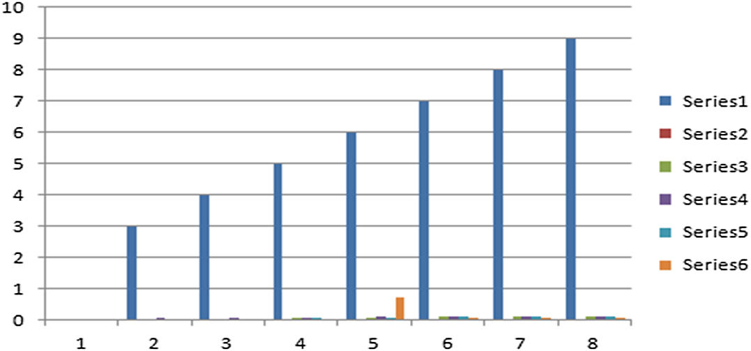Fig. 1. Graphical representation of the data shown in Table II.

In the following, we see the effect of the parameter $p$ on the DM results. It is clear from Table III that aggregation results obtained for Cq-ROFLWMM operator are almost same for distinct values of parameter $“ p . ”$ The ranking result for $p = (1, 0, 0, 0)$ is $Ѧ_{2} > Ѧ_{4} > Ѧ_{1} > Ѧ_{3}$ , whereas for $p = (1, 1, 0, 0)$ is $Ѧ_{2} > Ѧ_{1} > Ѧ_{4} > Ѧ_{3}$ , which is slightly distinct from above given ranking result, but the best result is same in both cases. The parameter $“ p ”$ can express the interrelationship among the independent arguments. For Cq-ROFLWMM, we can observe from Table III that if more interrelationship is considered among the attributes, SVs become smaller. The graphical representation of data given in Table III is shown in Fig. 2.

Fig. 2. Graphical representations of data shown in Table III.

D.COMPARATIVE ANALYSIS

In this section, we discuss the comparison of some other methods with established method and explore the superiority of the established work.

Example 2:A company board of directors decided to invest with other companies to increase its income. There are four companies $Ѧ_{1} = Textile company, Ѧ_{2} = Mobile company, Ѧ_{3} = Fertilizer company, and Ѧ_{4} = Cement company$ as alternative with four attributes given by $Ƀ_{1} = Risk analysis, Ƀ_{2} = Growth condition, Ƀ_{3} = Socia political impact,$ and $Ƀ_{4} = Environmental impact$ . Then, $w = (0.22, 0.26, 0.34, 0.18)$ is the WV of these alternatives. A few experts are said to assess these departments with the LTs set $S = {s_{o} = extremely low, s_{1} = very low, s_{2} = low, s_{3} = medium, s_{4} = high, s_{5} = very high, s_{6} = extxemely high}$ . The above four alternatives are evaluated using the cubic IF linguistic (CIFL) data given in Table IV.

TABLE IV CIFL INFORMATION

	$Ƀ_{1}$	$Ƀ_{2}$	$Ƀ_{3}$	$Ƀ_{4}$
$Ѧ_{1}$	$(\begin{matrix} s_{3}, (\begin{matrix} [0.50, 0.60], \\ [0.10, 0.20] \end{matrix}), \\ (0.40, 0.20) \end{matrix})$	$(\begin{matrix} s_{4}, (\begin{matrix} [0.20, 0.30], \\ [0.40, 0.50] \end{matrix}), \\ (0.30, 0.20) \end{matrix})$	$(\begin{matrix} s_{4}, (\begin{matrix} [0.40, 0.60], \\ [0.20, 0.30] \end{matrix}), \\ (0.20, 0.35) \end{matrix})$	$(\begin{matrix} s_{5}, (\begin{matrix} [0.40, 0.55], \\ [040, 0.50] \end{matrix}), \\ (0.30, 0.40) \end{matrix})$
$Ѧ_{2}$	$(\begin{matrix} s_{2}, (\begin{matrix} [[0.20, 0.30]], \\ [0.40, 0.50] \end{matrix}), \\ (0.40, 0.60) \end{matrix})$	$(\begin{matrix} s_{3}, (\begin{matrix} [0.15, 0.25], \\ [0.30, 0.35] \end{matrix}), \\ (0.20, 0.30) \end{matrix})$	$(\begin{matrix} s_{4}, (\begin{matrix} [0.20, 0.40], \\ [0.10, 0.20] \end{matrix}), \\ (0.40, 0.50) \end{matrix})$	$(\begin{matrix} s_{5}, (\begin{matrix} [0.30, 0.35], \\ [0.20, 0.30] \end{matrix}), \\ (0.45, 0.35) \end{matrix})$
$Ѧ_{3}$	$(\begin{matrix} s_{3}, (\begin{matrix} [[0.50, 0.60]], \\ [0.20, 0.30] \end{matrix}), \\ (0.20, 0.40) \end{matrix})$	$(\begin{matrix} s_{5}, (\begin{matrix} [0.40, 0.60], \\ [0.25, 0.35] \end{matrix}), \\ (0.30, 0.40) \end{matrix})$	$(\begin{matrix} s_{2}, (\begin{matrix} [0.50, 0.70], \\ [0.10, 0.15] \end{matrix}), \\ (0.30, 0.50) \end{matrix})$	$(\begin{matrix} s_{4}, (\begin{matrix} [0.10, 0.30], \\ [0.50, 0.60] \end{matrix}), \\ (0.20, 0.40) \end{matrix})$
$Ѧ_{4}$	$(\begin{matrix} s_{1}, (\begin{matrix} [0.30, 0.50], \\ [0.10, 0.30] \end{matrix}), \\ (0.10, 0.40) \end{matrix})$	$(\begin{matrix} s_{3}, (\begin{matrix} [0.40, 0.55], \\ [0.15, 0.20] \end{matrix}), \\ (0.30, 0.40) \end{matrix})$	$(\begin{matrix} s_{4}, (\begin{matrix} [0.40, 0.50], \\ [0.20, 0.30] \end{matrix}), \\ (0.45, 0.35) \end{matrix})$	$(\begin{matrix} s_{5}, (\begin{matrix} [0.23, 0.50], \\ [0.21, 0.40] \end{matrix}), \\ (0.30, 0.40) \end{matrix})$

CIFL weighted MM (CIFLWMM) and CPF linguistic MM (CPFLMM) operators are the particular cases of Cq-ROFLWMM, because for $q = 1$ , we have CIFLWMM operator, and for $q = 2$ , we have CPF linguistic weighted MM (CPFLWMM) operator. So here, we compare the established work in this paper with CIFLWMM and CPFLWMM operators. The ranking orders are given in Table V.

TABLE V RANKING RESULTS USING THE DISTINCT METHODS

Methods	Score values	Ranking results
CIFLWMM	$S (α_{1}) = 0.347018, S (α_{2}) = 0.300813, S (α_{3}) = 0.304032, S (α_{4}) = 0.295349$	$Ѧ_{1} > Ѧ_{3} > Ѧ_{2} > Ѧ_{4}$
CPFLWMM	$S (α_{1}) = 0.369267, S (α_{2}) = 0.322798, S (α_{3}) = 0.325699, S (α_{4}) = 0.312657$	$Ѧ_{1} > Ѧ_{3} > Ѧ_{2} > Ѧ_{4}$
Cq-ROFLWMM in this paper	$S (α_{1}) = 0.345848, S (α_{2}) = 0.308256, S (α_{3}) = 0.310386, S (α_{4}) = 0.293026$	$Ѧ_{1} > Ѧ_{3} > Ѧ_{2} > Ѧ_{4}$

From Table V, we observe that all ranking results are same for the above given CIFL information, which prove the validity of the proposed work. The graphical representation of these results is shown in Fig. 3.

Example 3:A company board of directors decided to invest with other companies to increase its income. There are four companies $Ѧ_{1} = Textile company, Ѧ_{2} = Mobile company, Ѧ_{3} = Fertilizer company, and Ѧ_{4} = Cement company$ as alternative with four attributes given by $Ƀ_{1} = Risk analysis, Ƀ_{2} = Growth condition, Ƀ_{3} = Socia political impact,$ and $Ƀ_{4} = Environmental impact$ . Then, $w = (0.23, 0.25, 0.32, 0.20)$ is the WV of these alternatives. A few experts are said to assess these departments with the LTs set $S = {s_{o} = extremely low, s_{1} = very low, s_{2} = low, s_{3} = medium, s_{4} = high, s_{5} = very high, s_{6} = extremely high}$ . The above four alternatives are evaluated using the CPFL information given in Table VI.

TABLE VI CPFL INFORMATION

	$Ƀ_{1}$	$Ƀ_{2}$	$Ƀ_{3}$	$Ƀ_{4}$
$Ѧ_{1}$	$(\begin{matrix} s_{3}, (\begin{matrix} [0.3, 0.4], \\ [0.7, 0.8] \end{matrix}), \\ (0.5, 0.8) \end{matrix})$	$(\begin{matrix} s_{4}, (\begin{matrix} [0.6, 0.7], \\ [0.5, 0.7] \end{matrix}), \\ (0.6, 0.7) \end{matrix})$	$(\begin{matrix} s_{4}, (\begin{matrix} [0.8, 0.9], \\ [0.3, 0.4] \end{matrix}), \\ (0.7, 0.5) \end{matrix})$	$(\begin{matrix} s_{5}, (\begin{matrix} [0.4, 0.8], \\ [0.5, 0.6] \end{matrix}), \\ (0.9, 0.4) \end{matrix})$
$Ѧ_{2}$	$(\begin{matrix} s_{2}, (\begin{matrix} [[0.8, 0.9]], \\ [0.3, 0.4] \end{matrix}), \\ (0.8, 0.6) \end{matrix})$	$(\begin{matrix} s_{3}, (\begin{matrix} [0.4, 0.8], \\ [0.5, 0.6] \end{matrix}), \\ (0.3, 0.9) \end{matrix})$	$(\begin{matrix} s_{4}, (\begin{matrix} [0.7, 0.8], \\ [0.4, 0.5] \end{matrix}), \\ (0.9, 0.3) \end{matrix})$	$(\begin{matrix} s_{5}, (\begin{matrix} [0.5, 0.6], \\ [0.7, 0.8] \end{matrix}), \\ (0.7, 0.5) \end{matrix})$
$Ѧ_{3}$	$(\begin{matrix} s_{3}, (\begin{matrix} [[0.4, 0.5]], \\ [0.7, 0.8] \end{matrix}), \\ (0.3, 0.9) \end{matrix})$	$(\begin{matrix} s_{5}, (\begin{matrix} [0.5, 0.6], \\ [0.7, 0.8] \end{matrix}), \\ (0.8, 0.4) \end{matrix})$	$(\begin{matrix} s_{2}, (\begin{matrix} [0.6, 0.8], \\ [0.5, 0.6] \end{matrix}), \\ (0.6, 0.7) \end{matrix})$	$(\begin{matrix} s_{4}, (\begin{matrix} [0.6, 0.7], \\ [0.5, 0.7] \end{matrix}), \\ (0.8, 0.6) \end{matrix})$
$Ѧ_{4}$	$(\begin{matrix} s_{1}, (\begin{matrix} [0.6, 0.7], \\ [0.4, 0.5] \end{matrix}), \\ (0.9, 0.4) \end{matrix})$	$(\begin{matrix} s_{3}, (\begin{matrix} [0.3, 0.4], \\ [0.8, 0.9] \end{matrix}), \\ (0.7, 0.6) \end{matrix})$	$(\begin{matrix} s_{4}, (\begin{matrix} [0.5, 0.6], \\ [0.7, 0.8] \end{matrix}), \\ (0.9, 0.4) \end{matrix})$	$(\begin{matrix} s_{5}, (\begin{matrix} [0.3, 0.4], \\ [0.8, 0.9] \end{matrix}), \\ (0.5, 0.8) \end{matrix})$

CIFLWMM and CPFLMM operators are the special cases of Cq-ROFLWMM, because for $q = 1$ , we have cubic IF weighted MM (CIFWMM) operator, and for $q = 2$ , we have CPF weighted MM (CPFWMM) operator. So here, we compare the established work with CIFLWMM and CPFWMM operators. The ranking results are given in Table VII. The graphical representation of these results is shown in Fig. 4.

TABLE VII RANKING RESULTS USING DIFFERENT METHODS

Methods	Score values	Ranking results
CIFLWMM	cannot be calculated	Cannot be calculated
CPFLWMM	$S (α_{1}) = 0.365082$ , $S (α_{2}) = 0.371129$ , $S (α_{3}) = 0.313622$ , $S (α_{4}) = 0.315955$	$Ѧ_{2} > Ѧ_{1} > Ѧ_{4} > Ѧ_{3}$
Cq-ROFLWMM in this paper	$S (α_{1}) = 0.378759$ , $S (α_{2}) = 0.386831$ , $S (α_{3}) = 0.325856$ , $S (α_{4}) = 0.33006$	$Ѧ_{2} > Ѧ_{1} > Ѧ_{4} > Ѧ_{3}$

From Table VII, we can see that ranking results are same for the above-given information in the form of CPFL information, which shows the validity of proposed Cq-ROFLWMM operator. Since CIFLMM operator can only deal with CIFL information, CIFL information also involves the CIF information which has the condition that $0 \leq ч + ѵ \leq 1$ for IFSs and $0 \leq ч^{U} + ѵ^{U} \leq 1$ for IVIFSs. However, when the decision-maker gives the information as $(\begin{matrix} s_{5}, (\begin{matrix} [0.5, 0.6], \\ [0.7, 0.8] \end{matrix}), \\ (0.8, 0.4) \end{matrix}),$ then the above-given condition fails to hold with such type of information, but the proposed work can deal with such type of information. Therefore, Cq-ROFLWMM operator in this paper is superior than CIFLWMM operator.

Example 4:A company board of directors decided to invest with other company to increase its income. There are four companies $Ѧ_{1} = Textile company, Ѧ_{2} = Mobile company, Ѧ_{3} = Fertilizer company, and Ѧ_{4} = Cement company$ as alternative with four attributes given by $Ƀ_{1} = Risk analysis, Ƀ_{2} = Growth condition, Ƀ_{3} = Socia political impact,$ and $Ƀ_{4} = Environmental impact$ . Then, $w = (0.21, 0.27, 0.30, 0.22)$ is the WV of these alternatives. A few experts are said to assess these departments with the LTs set $S = {s_{o} = extremely low, s_{1} = very low, s_{2} = low, s_{3} = medium, s_{4} = high, s_{5} = very high, s_{6} = extremely high}$ . The above four alternatives are evaluated using the Cq-ROFL information given in Table VIII.

TABLE VIII CQ-ROFL INFORMATION

	$Ƀ_{1}$	$Ƀ_{2}$	$Ƀ_{3}$	$Ƀ_{4}$
$Ѧ_{1}$	$(\begin{matrix} s_{3}, (\begin{matrix} [0.5, 0.9], \\ [0.5, 0.6] \end{matrix}), \\ (0.5, 0.7) \end{matrix})$	$(\begin{matrix} s_{4}, (\begin{matrix} [0.6, 0.9], \\ [0.4, 0.5] \end{matrix}), \\ (0.6, 0.7) \end{matrix})$	$(\begin{matrix} s_{4}, (\begin{matrix} [0.6, 0.7], \\ [0.6, 0.8] \end{matrix}), \\ (0.8, 0.5) \end{matrix})$	$(\begin{matrix} s_{5}, (\begin{matrix} [0.6, 0.9], \\ [0.6, 0.6] \end{matrix}), \\ (0.5, 0.8) \end{matrix})$
$Ѧ_{2}$	$(\begin{matrix} s_{2}, (\begin{matrix} [[0.5, 0.8]], \\ [0.6, 0.7] \end{matrix}), \\ (0.5, 0.6) \end{matrix})$	$(\begin{matrix} s_{3}, (\begin{matrix} [0.7, 0.9], \\ [0.5, 0.6] \end{matrix}), \\ (0.7, 0.8) \end{matrix})$	$(\begin{matrix} s_{4}, (\begin{matrix} [0.5, 0.8], \\ [0.3, 0.6] \end{matrix}), \\ (0.5, 0.7) \end{matrix})$	$(\begin{matrix} s_{5}, (\begin{matrix} [0.7, 0.7], \\ [0.5, 0.8] \end{matrix}), \\ (0.7, 0.6) \end{matrix})$
$Ѧ_{3}$	$(\begin{matrix} s_{3}, (\begin{matrix} [[0.8, 0.9]], \\ [0.5, 0.6] \end{matrix}), \\ (0.6, 0.9) \end{matrix})$	$(\begin{matrix} s_{5}, (\begin{matrix} [0.6, 0.7], \\ [0.3, 0.6] \end{matrix}), \\ (0.5, 0.7) \end{matrix})$	$(\begin{matrix} s_{2}, (\begin{matrix} [0.5, 0.6], \\ [0.4, 0.7] \end{matrix}), \\ (0.8, 0.7) \end{matrix})$	$(\begin{matrix} s_{4}, (\begin{matrix} [0.5, 0.6], \\ [0.8, 0.9] \end{matrix}), \\ (0.6, 0.7) \end{matrix})$
$Ѧ_{4}$	$(\begin{matrix} s_{1}, (\begin{matrix} [0.5, 0.7], \\ [0.5, 0.6] \end{matrix}), \\ (0.7, 0.6) \end{matrix})$	$(\begin{matrix} s_{3}, (\begin{matrix} [0.5, 0.6], \\ [0.7, 0.8] \end{matrix}), \\ (0.7, 0.6) \end{matrix})$	$(\begin{matrix} s_{4}, (\begin{matrix} [0.7, 0.8], \\ [0.5, 0.6] \end{matrix}), \\ (0.4, 0.7) \end{matrix})$	$(\begin{matrix} s_{5}, (\begin{matrix} [0.6, 0.8], \\ [0.5, 0.7] \end{matrix}), \\ (0.6, 0.7) \end{matrix})$

CIFLWMM and CPFLMM operators are the special cases of Cq-ROFLWMM, because for $q = 1$ , we have CIFWMM operator, and for $q = 2$ , we have CPFWMM operator. So here, we compare the established work with CIFLWMM and CPFWMM operators. The ranking results are given in Table IX.

TABLE IX RANKING RESULTS USING DIFFERENT METHODS

Methods	Score values	Ranking results
CIFLWMM	Cannot be calculated	Cannot be calculated
CPFLWMM	Cannot be calculated	Cannot be calculated
Cq-ROFLWMM in this paper	$S (α_{1}) = 0.362769$ , $S (α_{2}) = 0.346287$ , $S (α_{3}) = 0.323648$ , $S (α_{4}) = 0.309693$	$Ѧ_{1} > Ѧ_{2} > Ѧ_{3} > Ѧ_{4}$

From Table IX, we can observe that CIFLWMM and CPFLWMM operators cannot deal with the information given above, because when decision maker provides information in the form of $(\begin{matrix} s_{3}, (\begin{matrix} [[0.8, 0.9]], \\ [0.5, 0.6] \end{matrix}), \\ (0.6, 0.9) \end{matrix})$ , then the CIFLWMM and CPFLWMM operators fail to tackle such kind of information, but proposed work can deal with this type of information. Therefore, established method is superior. Also, Cq-ROFLWMM operator can consider the interrelation structure between all the input arguments. The graphical representation of these results is given in Fig. 5.

Fig. 3. Graphical representation of data comparison shown in Table V.

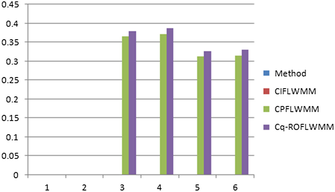Fig. 4. Graphical representation of data comparison shown in Table VII.

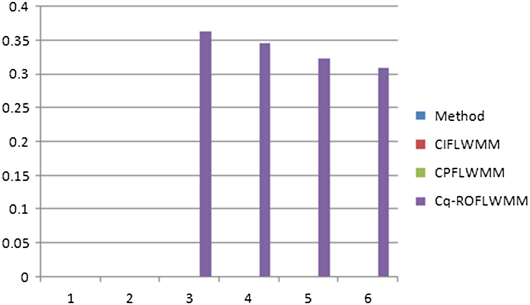Fig. 5. Graphical representation of data comparison shown in Table IX.

VI.CONCLUSION

Cq-ROFS is a mixture of two different notions like IVq-ROFS and q-ROFS to manage the vague and complicated facts in FS theory. Cq-ROFS contains MD and NMD as a single and also in the form of interval, whose constraint is that the sum of MD and NMD is limited to [0,1]. Due to the powerful structure of Cq-ROFS and the concept of linguistic variables, in this paper, we have established the idea of Cq-ROFLS, which is qualitative form of Cq-ROFSs to deal with MADM problems. Under this developed set, we formulate the new Cq-ROFLMM operator and its weighted form as Cq-ROFLWMM operator. Furthermore, Cq-ROFLDMM operator and its weighted form as Cq-ROFLDWMM operator is discussed later, and the properties of these operators are explored. The most remarkable property of these operators is that they can consider the interrelationship between multiple attributes. Keeping in view the advantages of the established operators, we have solved a numerical example in MADM problems using the environment of Cq-ROFL information to evaluate the superiority and effectiveness of the established approaches. The comparative analysis, advantages, and graphical interpretation of the established work with existing drawbacks are also discussed in detail to verify the reliability and validity of the explored work.

In the future, there is a scope of elongating the research to some uncertain linguistic environment [37]. In addition, we will define some more generalized algorithms to solve more complex problems, such as brain hemorrhage, healthcare, nonlinear systems, control systems, and others [38], [39].

Cubic q-Rung Orthopair Fuzzy Linguistic Set and Their Application to Multiattribute Decision-making with Muirhead Mean Operator

I.INTRODUCTION

II.PRELIMINARIES

III.CQ-ROFLS

IV.CQ-ROFLMM OPERATOR

V.MODEL FOR MADM WITH CQ-ROFL INFORMATION

A.PROPOSED ALGORITHM

B.ILLUSTRATIVE EXAMPLE

C.THE EFFECT OF THE PARAMETERS p AND q ON RANKING RESULTS

D.COMPARATIVE ANALYSIS

VI.CONCLUSION

REFERENCES