JAIT

I.INTRODUCTION

Due to growing consumer awareness of environmental protection and energy conservation, as well as rising fuel prices, there is an increasing interest in new energy vehicles (NEVs) [1]. Additionally, the government’s active promotion and publicity of NEVs has further raised consumer awareness and acceptance of these vehicles. As the public recognizes NEVs, their sales have increased annually, leading to a rise in the number of charging piles (CPs) for NEVs in the city [2]. However, this increase in CPs has also brought about safety hazards. The voltage of CP can reach 770 V, which poses a significant safety hazard during its use. Additionally, the internal metal parts of CP cannot be completely grounded, increasing the risk of electric shock. Effectively predicting and avoiding CP failures has become an urgent problem [3]. The gated recurrent unit (GRU) network is currently widely used in various prediction models due to its fast convergence and high accuracy. One popular optimization technique in the deep learning space is the whale optimization algorithm (WOA) [4]. It can compensate for the local optimization shortcomings of the GRU algorithm [5]. This research combines the above two algorithms to create a new charging pile failure prediction (CPFP) model. There are two innovative designs in this study: (1) GRU network is used as the core algorithm of the model, which can solve the deficiency of traditional prediction models that rely on a large number of training samples and (2) research on using WOA algorithm to improve the weak global search ability of GRU network.

The rest of the paper is structured as follows. The second section introduces the relevant work, which mainly summarizes the current development and application of GRU and WOA algorithms. The third section introduces the method of model construction, which describes the construction and optimization process of the CP fault prediction model. The fourth section introduces the performance test experiment of the model, which verifies the progressiveness of the proposed model through comparative experiments. Finally, conclusion section summarizes the research results and identifies the shortcomings of this study.

II.RELATED WORKS

Both GRU and WOA are commonly used research methods for intelligent models in recent years, and at this stage, many researchers have made improvements and optimizations for both algorithms. Xia M et al. found that the intelligent forecasting model is still challenging under the influence of user behavior when studying the forecasting of electric load. In order to estimate renewable energy generation and electrical load in univariate and multivariate scenarios, Xia M et al. suggested a modified stacked gated recurrent unit recurrent neural network (GRU-RNN). In terms of attaining precise energy prediction for efficient smart grid operation, the suggested approach has been proven to be cutting edge and even more successful than cutting-edge machine learning techniques [6]. A category-aware gated recurrent unit model, ATCA-GRU, was proposed by Liu Y et al. The model mitigates the adverse effects of sparse check-in data and captures the long-term dependency of user check-ins through a gate control mechanism. The model was tested on Foursquare’s real-world dataset, and the experimental results showed that the ATCA-GRU model outperforms existing similar approaches for next Point of Interest (POI) recommendation [7]. Li Y et al. developed a composite GRU–Prophet model for sales prediction that includes an attention mechanism. The study’s suggested model, which has been shown through experimentation to be more accurate than a similar kind of prediction model, is therefore appropriate for the quick changes in consumer demand and boosts a company’s ability to compete in the smart manufacturing space [8]. Hamayel M J and other researchers found that the price prediction of cryptocurrencies is very difficult to rely on human labor by studying the volatility and dynamics of their prices, so a new prediction model based on gated recursive units is proposed. The model can fit the cryptocurrency price transformation curve and make predictions based on the existing trends. The findings revealed that the results of the proposed prediction model are very close to the accurate results of the actual price of cryptocurrencies, and the correct prediction rate is higher than that of other similar models, thus verifying the feasibility and advancement of the proposed model [9]. Abdelgwad M M and other researchers have implemented a fine-grained analysis of sentiment analysis (ABSA). With a 39.7% higher F1 score for opinion target extraction and 7.58% greater accuracy for aspect-based sentiment polarity classification when compared to the control model, the experimental findings showed that the model is state-of-the-art [10].

Zhang J and other researchers combined WOA and woodpecker mating algorithm (WMA) into Hybrid Woodpecker and Whale Optimization Algorithm (HWMWOA) and proposed an engineering design optimization algorithm based on HWMWOA. By refining the parameters of the support vector machine and feature weighting, the HWMWOA improved the model’s performance and overcame the shortcomings of WOA, which is prone to local optimal convergence, miss population diversity, and converge too soon. It was experimentally verified that the proposed model significantly outperforms other effective techniques and has good scalability, which can provide a valuable reference for subsequent research [11]. Chakraborty S et al. found that the WOA optimization algorithm has excellent performance on a wide range of optimization problems but also increases the probability of premature convergence and therefore proposed a new modified WOA (m-SDWOA). The method introduced a new selection parameter for choosing between the exploration and exploitation phases of the algorithm, thus balancing the ability of the algorithm to explore or exploit. The optimization seeking ability of the model was verified through four real-world engineering design problems, and the results showed the superiority of the proposed algorithm with respect to the comparative algorithms [12]. Husnain G and other researchers proposed an efficient clustering technique for route optimization in intelligent transportation systems (ITSs) in order to solve the problem of highly mobile vehicles with rapidly changing topology that makes it difficult to maintain routes for all vehicles in the network. The technique minimized randomness using the WOA and enables diversity in route optimization for transportation systems. The outcomes of the study revealed that the proposed model effectively reduces the communication cost and routing overhead while generating the optimal cluster heads, which is state-of-the-art [13]. Dai Y et al. suggested a new whale optimization algorithm (NWOA). By introducing a potential field factor, this method was able to tackle the issues of poor convergence speed and lack of dynamic obstacle avoidance capabilities of WOA. The NWOA model has higher dynamic planning and faster convergence in mobile robot path planning, according to the experimental data [14]. Lu Y and other researchers proposed a short-term load forecasting model based on support vector regression (SVR) and WOA in order to forecast electricity load. The model considered the influence of real-time electricity price and introduces the chaos mechanism and adversarial learning strategy to balance the parameters of the algorithm. It was experimentally proved that the proposed model possesses better prediction ability and faster convergence speed compared with SVR and Back Propagation Neural Network (BPNN) models [15].

In summary, many research works have been devoted to developing effective CPFP models in recent years. Traditional machine learning and statistical techniques like random forests, time series analysis, and support vector machines form the foundation of the majority of these models. However, due to the temporal and nonlinear nature of CP fault data, traditional methods often fail to accurately capture these characteristics, resulting in poor prediction accuracy. According to the research results of Xia M et al., although the current improved GRU network has a good prediction mechanism, it has the disadvantage of difficult global convergence. In order to solve the problem of difficult convergence of GRU networks in recognition and prediction tasks, research has innovated the GRU network in a new direction by introducing global optimization algorithms for improvement. According to literature review, the WOA algorithm has a fast convergence speed and can compensate for the shortcomings of GRU networks. In view of this, the study proposes the idea of combining GRU network with WOA algorithm. After introducing the WOA algorithm, the position sharing mechanism of fish schools can enable the GRU network to quickly preview global information. Therefore, the GRU network optimized based on the WOA algorithm has faster convergence ability than the current ordinary optimized GRU model. The innovation of the research mainly focuses on optimizing the global parameter sharing mechanism of GRU networks, using the WOA algorithm to improve the ability of GRU networks to collect and integrate global parameters.

III.CONSTRUCTION OF CP FAULT DETECTION MODEL INTEGRATING GRU AND WOA

With the popularization of electric vehicles, the importance of CP as an infrastructure is becoming more and more prominent, and neural network-based models are widely used for CP fault detection in existing research. This study addresses the problem of automated CP fault detection to construct an efficient and accurate model, aiming to ensure safety during vehicle charging and promote the development of NEVs.

A.GRU-BASED CP FAULT ALARM MODELING STUDY

The GRU algorithm is evolved from the Long Short-Term Memory Network (LSTM) algorithm, and through integration and optimization, the GRU algorithm effectively solves the deficiencies of the LSTM algorithm in terms of parallel processing capability and training time [17]. GRU algorithm is a kind of artificial neural network model with simple structure and fewer training parameters, but it shows strong learning ability when learning and training on small amount of data [18]. High efficiency, adaptability, and scalability are other benefits of the GRU algorithm that make it a popular tool in the machine learning space. Fig. 1 depicts the GRU algorithm’s structure.

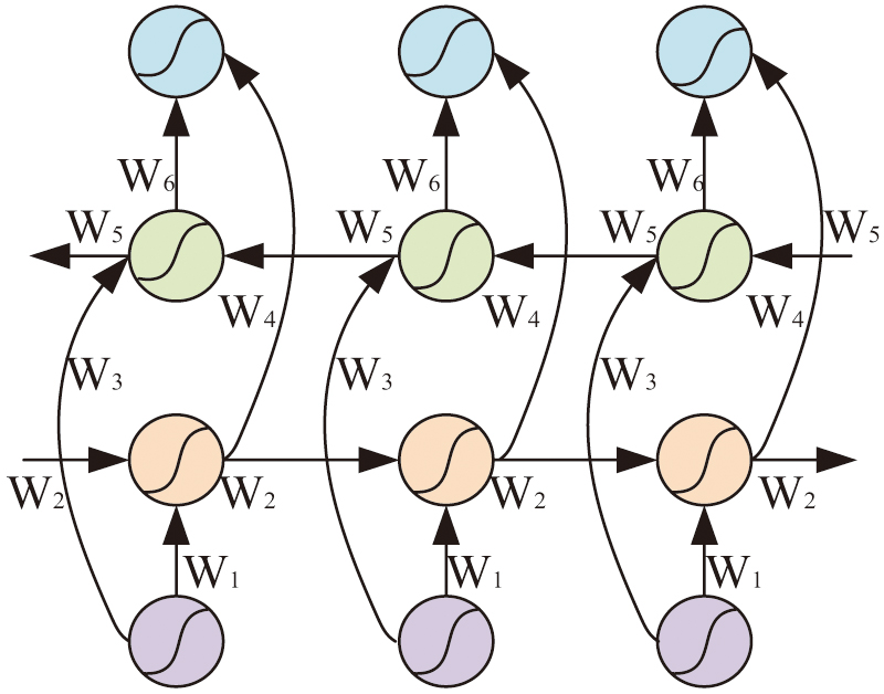Fig. 1. Structure diagram of GRU algorithm.

The GRU algorithm has a unique “oblivion gate” system, which constitutes the prediction unit through the synergistic action with input gate (IG) and output gate (OG), as well as the interaction with internal memory cells [19]. In the GRU algorithm, the design of the forgetting gate (FG) can effectively clear the old information and make room for new information. Thus, the GRU model can prevent overfitting, enhance the model’s capacity for generalization, and more readily adjust to fresh input data. Fig. 2 illustrates the gate control structure of the GRU algorithm, which consists of an IG, an OG, and an FG. Where $r_{t}$ denotes the reset gate and the table update gate. $α$ is the activation function of the algorithm, and $h_{t}$ is the hidden layer state parameter. $X$ denotes the position information.

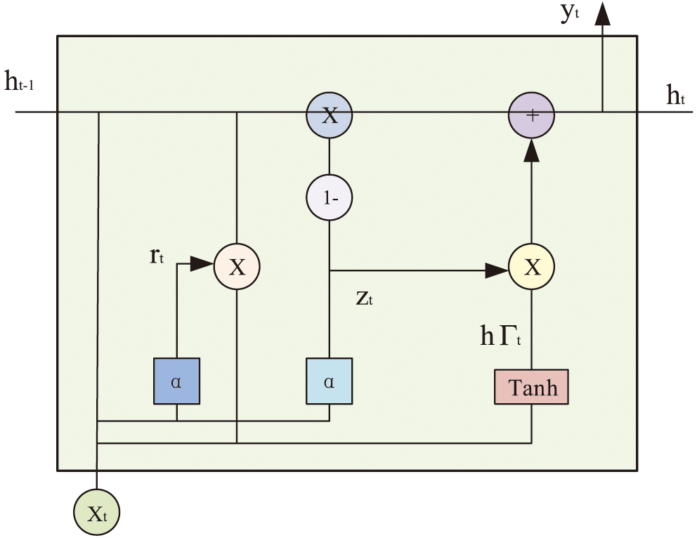Fig. 2. Door control structure diagram.

The algorithm filters the historical information of the prediction unit through the FG, and its filtering calculation is shown in equation (1):

f_{t} = α (W_{f} x_{t} + W_{o} h_{t - 1} + b_{f})

(1)

In equation (1), $W_{f}$ is the weight matrix (WM) of the FG and $W_{o}$ is the WM of the IG. $α$ is the computation parameter with the value range of [0,1]. $x_{t}, h_{t - 1}$ is the hidden layer state vector parameter, and $b_{f}$ is the bias vector. The filtered information will be multiplied bit by bit with the elements in the unit state $U_{t}$ , and when the value of $f_{t}$ is 0, the relevant information in $U_{t - 1}$ will be zeroed out, thus leaving more space. When the value of $f_{t}$ is 1, all relevant information in $U_{t - 1}$ will be retained. This calculation is a selective retention of past information. The role of the IG is then to selectively preserve the new information and update the $U_{t}$ after performing the calculation. The formula for the $U_{t}$ update is shown in equation (2):

{\begin{cases} i_{t} = α (W_{f} x_{i} + W_{i} h_{t - 1} + b_{i}) \\ g_{t} = Tanh (W_{g} x_{t} + W_{i} h_{t - 1} + b_{g}) \\ c_{t} = f_{t} \cdot U_{t - 1} + i_{t} \cdot g_{t} \end{cases}

(2)

In equation (2), $W_{g}$ is the WM of the FG and $W_{i}$ is the WM of the IG. $b_{g}$ is the IG bias vector. $Tanh (.)$ is the hyperbolic tangent function, that is, the hyper-tangent function. $i_{t}, g_{t}$ is the update information of the FG and the IG, respectively. At this time the prediction unit state $U_{t}$ has updated the memory unit output, the output of time step is shown in equation (3):

o_{t} = α (W_{o} x_{t} + W_{g} h_{t - 1} + b_{0})

(3)

In equation (3), $o_{t}$ is the output result of the OG and $b_{o}$ is the bias vector of the OG. $W_{o}$ is the WM of the OG. The output result of $h_{t}$ is obtained from $o_{t}$ with the new cell state after contraction by the $Tanh$ function, which is calculated as shown in equation (4):

h_{t} = o_{t} \cdot Tanh (U_{t})

(4)

By using the above formula, it can be found that when the GRU network carries out information transmission, its predictive unit states $U_{t}$ , $U_{t - 1}$ and the lower line to transfer information between the hidden state units $h_{t}$ , $h_{t - 1}$ all show a linear self-loop relationship. This linear self-recycling relationship implies that there is a direct dependency between the current state and the previous state in the GRU network, that is, the current state is affected by the previous state, and this effect is transmitted through a linear function [20]. After integrating the FG, IG as well as the OG, the formula for the reset gate calculation in the GRU network structure is shown in equation (5):

r_{t} = β (W_{r} x_{t} + S_{r} h_{t - 1} + b_{r})

(5)

In equation (5), $W_{r}$ and $S_{r}$ denote the deep feature WM collected by the sensor. $b_{r}$ denotes the bias vector of the car charging data and $β$ is the activation function. $r_{t}$ is the output of the reset gate. The main role of the reset gate is to control the extent to which previous information is forgotten; by adjusting the value of the reset gate, it is possible to decide which historical states need to be retained and which need to be forgotten. The introduction of reset gates can improve the utilization of storage space and ensure better utilization of information not stored in memory. The storage space can be utilized more efficiently with the help of reset gates, which improves the utilization of the storage space. In addition, the update gate in GRU network also has a huge impact on the information processing of the network, and the formula for the update gate is shown in equation (6):

z_{t} = β (W_{z} x_{t} + S_{z} h_{t - 1} + b_{z})

(6)

In equation (6), $b_{z}$ is the bias vector of the update gate, $S_{z}$ is the update gate WM, and $b_{z}$ is the update gate bias vector. The update gate’s function is to regulate whether the model retains memory of the prior state data and how the new input data is combined with the prior state data. There is an update gate at each time step in the GRU network, which is usually computed using the sigmoid function, and the update gate output value is a constant between [0,1]. The GRU algorithm operation flow is shown in Fig. 3.

Fig. 3. GRU algorithm running process.

The gating mechanism in the GRU algorithm has the advantages of capturing long-term dependencies, improving efficiency, alleviating the gradient vanishing problem, and fusing short-term and long-term memory. These features make GRU have excellent performance and performance in processing sequence data.

B.CONSTRUCTION OF FAULT JUDGMENT MODEL BY INTEGRATING GRU AND WOA

The WOA originates from the whale population foraging process and is a type of merit selection algorithm, which is commonly used to optimize various types of neural networks [21]. The algorithm is divided into three processes: searching for prey, encircling food, and blister net hunting. The searching for prey phase involves finding the position of each whale and updating it in real time, which is determined by the positions of different individuals randomly selected from the hunting group [22]. By randomly selecting out individuals to represent the whole population, the emergence of local optimal solutions can be effectively avoided, and the upper limit of the algorithm’s optimization search can be improved. The formula for updating the position information of random individuals is shown in equation (7):

X (t + 1) = X_{r a n d} (t) - λ D

(7)

In equation (7), $X_{r a n d} (t)$ is the current position of the selected random individual, and $λ$ is the coefficient vector, which can be set by ourselves. $t$ is the number of iterations. $X (t + 1)$ denotes the position of the individual at the next time. $D$ is the distance between the unselected individual and the randomly selected individual. The computational expression of $D$ is shown in equation (8):

D = | ζ X_{r a n d} (t) - X (t) |

(8)

In equation (8), $ζ$ denotes the vector of coefficients at the current position and $| . |$ here denotes the absolute value taken. The search for prey process also increases the robustness of the algorithm through the mechanism of whales swimming randomly and moving away from each other and other whales. The significance of this process is to find as many solutions as possible through global search and to find better solutions among them and to provide conditions for the whales to surround the food [23]. When individual whales find food, they conduct a localized search and focus on their prey. The position of the whale that finds the food is the closest to the food, and that position is updated to the optimal position, and the updated position is the closest to the optimal solution globally [24]. The other whales that have not found food optimally update their positions according to the distance from the food. The above process is the second stage of the WOA, and the whale position update calculation in this process is shown in equation (9):

X (t + 1) = X_{b e s t} - χ \cdot D

(9)

In equation (9), $X_{b e s t}$ denotes the location of the food and $X (t + 1)$ denotes the updated location information. $χ$ denotes the distance coefficient vector of the stage. $X$ is the current position of the whale. With the iterations increasing, the position of the whale that constantly finds the food is compared with the current optimal solution. If the two are not in the same position, the position of the current optimal solution needs to be re-updated, and if the two are the same, the iteration ends. At this time, the computational expression for the distance $D$ between the unselected individual and the randomly selected individual is shown in equation (10):

D = | ζ \cdot X_{b e s t} - X (t) |

(10)

In equation (10), $ζ$ denotes the distance coefficient vector of the second stage. This distance coefficient vector is different from the first stage, the first stage coefficient vector needs to be given by human, and the second stage coefficient vector has a model to calculate automatically. The calculation formula is shown in equation (11):

{\begin{cases} χ = 2 a r - a \\ ζ = 2 r \end{cases}

(11)

In equation (11), $r$ denotes a vector taking the value [0.1]. $a$ denotes a control parameter that varies with the number of iterations. The formula for the parameter $a$ is shown in equation (12):

a = 2 - 2 \frac{t}{T_{M A X}}

(12)

In equation (12), $T_{M A X}$ is the maximum iterations and $t$ is the current iterations. The distance between the present individual and the ideal location must be determined before moving on to the third stage of the WOA, known as bubble net hunting. The formula for this computation is provided in equation (13):

D_{n} = | X_{b e s t} - X (t) |

(13)

After getting the distance between the current individual and the best position construct a movement function based on the position of the two and the distance apart, the function takes the current whale position as the starting point and the best position as the end point. The movement function is mostly spiral, as shown in Fig. 4.

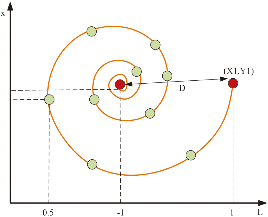Fig. 4. Schematic diagram of WOA spiral movement path.

The spiral movement function ensures the maximization of the individual whale’s range of motion as the individual moves toward the optimal position, further reducing the possibility of local convergence [25]. The mathematical expression of the spiral movement function is shown in equation (14):

Y (t + 1) = D_{n} \cdot e^{ϕ i} \cos (2 π θ) + X^{'} (t)

(14)

In equation (14), $ϕ$ denotes the logarithmic spiral shape. $θ$ denotes a uniformly distributed constant in the interval [–1,1]. $i$ denotes the individual whale serial number. $X^{'} (t)$ is a relative distance indicating the path distance of the individual from the optimal position at the $t$ th iteration. To avoid local optimization when the model is running, this study integrates the WOA with GRU to construct the GRU-WOA model. Fig. 5 displays the model operation’s flowchart.

Fig. 5. GRU-WOA flowchart.

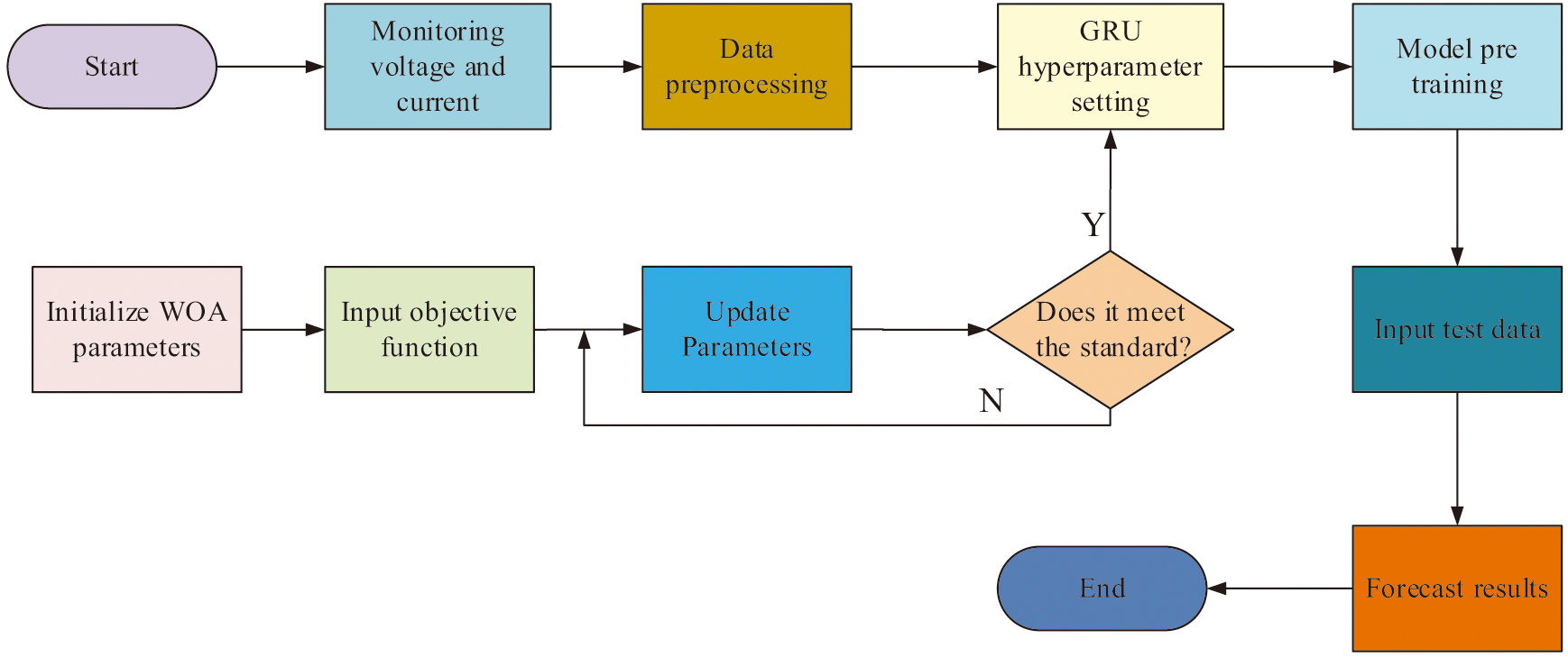
As a result, the construction of the CP fault detection model based on the WOA-GRU algorithm, referred to as the W-GRU model, is completed. The proposed model can prevent the damage of CP and extend its service life, thus reducing the cost of maintenance and replacement. It can also discover and solve the potential safety hazards of CP to protect the safety of users and maintenance personnel [26]. The fault warning process is shown in Fig. 6.

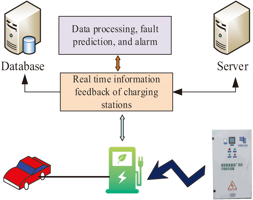Fig. 6. Schematic diagram of fault warning.

The fusion of GRU and WOA greatly improves the performance of the CP fault detection model so that users can avoid the inability to charge and other safety hazards caused by equipment failure during the process. The proposed model plays a facilitating role for the development and popularization of NEVs and also has a positive impact on energy saving and emission reduction.

IV.PERFORMANCE ANALYSIS OF FAULT DETERMINATION MODEL INCORPORATING GRU AND WOA

The relevant equipment and environment used for this validation experiment include a server with Intel Xeon toron-x5650 CPU, JavaSE compiler, JDK17. The datasets used for the experiment are CWRU dataset and PEDL dataset, and the comparative models are Stacked GRU-RNN and ATCA-GRU. To demonstrate the innovation of performance testing experiments, a multiple comparison method was used to analyze the performance of the model. On the same dataset, the research shows the progressiveness of the proposed algorithm according to the difference of model output results. Comparing the results of the same model on different datasets can test the stability and universality of the model.

First, the GRU-RNN and ATCA-GRU models are utilized as controls, while the CWRU and PEDL datasets are used as inputs to assess the accuracy of the suggested models. Fig. 7 displays the outcomes of the experiment. Fig. 7(a) represents the variation of accuracy versus training time for the three models on the CWRU dataset, where the average accuracy of the three models GRU-RNN, ATCA-GRU, and WOA-GRU are 86.71%, 84.92%, and 90.16%, respectively. Fig. 7(b) represents the variation of accuracy versus training time for the three models on the PEDL dataset, and the average accuracy of the three models GRU-RNN, ATCA-GRU, and WOA-GRU on this dataset is 82.11%, 76.50%, and 92.02%, respectively. Due to the relatively simple data samples in the CWRU dataset, the accuracy of each model on this dataset is higher than that on the PELD dataset.

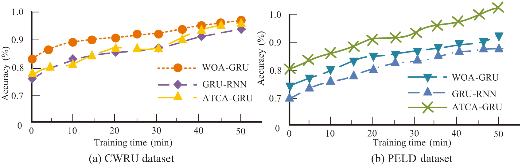Fig. 7. Comparison of accuracy on different datasets.

The ratio of lost samples to total samples in the model prediction results is known as the model loss rate. A high loss rate causes sample bias, which leads to inaccurate model prediction results. In this study, the CWRU dataset was used as input to compare the loss rates of three models, GRU-RNN, ATCA-GRU, and WOA-GRU, and the experimental process was repeated several times to calculate the average model loss rate results as shown in Fig. 8. Figure 8(a) shows the average loss rate curves of the three models following three iterations of the tests, whereas Fig. 8(b) shows the model’s loss rate curves during the first iteration of the experiment. According to the information in the figure, the WOA-GRU model has the lowest loss rate, and the average loss rate of the WOA-GRU model is more similar to the change trend of the first run of the lost dead, so the WOA-GRU model has higher stability and accuracy.

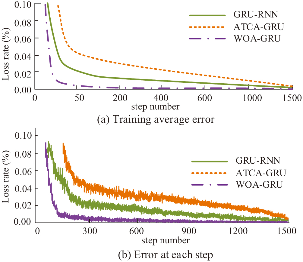Fig. 8. Schematic diagram of loss rate and average loss rate.

To observe the model’s prediction effect on CP faults more intuitively, this study compares the model training real values with the training predicted values. The CWRU dataset served as the experiment’s input dataset, and the GRU-RNN model served as the control model. Figure 9 displays the experimental findings. Figure 9(a) represents the results of comparing the training true values with the training predicted values for the WOA-GRU model, and Fig. 9(b) represents the results of comparing the training true values with the training predicted values for the GRU-RNN model. When Figs. 9(a) and 9(b) are compared, it can be seen that the WOA-GRU model’s predicted values are more closely aligned with the true values and have a greater prediction accuracy. Additionally, the predicted values are densely dispersed.

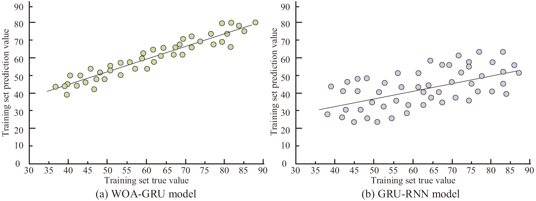Fig. 9. Comparison between the actual and predicted values of model training.

Recall and F1 value are both one of the important indicators for model detection, and this study uses the CWRU dataset as an input to compare the recall as well as the F1 value of the three models, GRU-RNN, ATCA-GRU, and WOA-GRU, and the results are shown in Fig. 10. Figure 10(a) represents the recall of the three models, from which it can be seen which model’s recall increases with the increase in the number of iteration steps, and the average values of the recall of the three models, GRU-RNN, ATCA-GRU, and WOA-GRU, are 77.68%, 74.95%, and 85.66%, respectively. Figure 10(b) represents the F1 values of the three models, from which it can be seen that the F1 values of the three models GRU-RNN, ATCA-GRU, and WOA-GRU are 88.79%, 86.03%, and 93.87% respectively. The F1 value of WOA-GRU model is much higher than the other two models, so the comprehensive performance of WOA-GRU model is better.

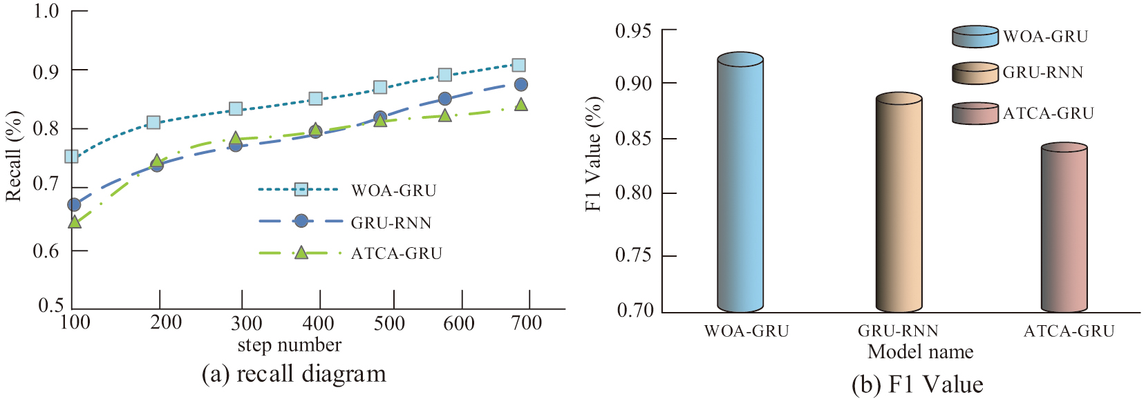Fig. 10. Schematic diagram of model recall rate and F1 value.

The true positive rate is the vertical coordinate on the Receiver Operating Characteristic (ROC) curve graph, which is used to assess the effectiveness of binary classifiers. The false positive rate is represented as the horizontal coordinate. The main advantage of the ROC curve is that the curve provides a complete view of the performance of the binary classifier at various possible thresholds. This study used the CWRU dataset as input to compare the ROC curves of the three models GRU-RNN, ATCA-GRU, and WOA-GRU. Figure 11 revealed the findings. The WOA-GRU model constitutes the largest area with respect to the reference line, and therefore this model performs better than the two control models.

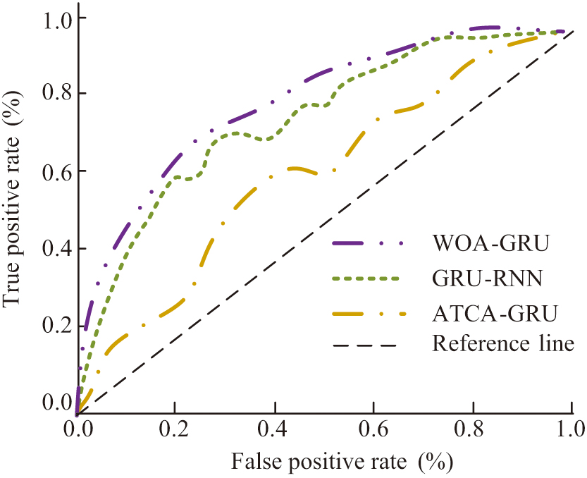Fig. 11. Schematic diagram of ROC curves for different models.

The running time can reflect the computational efficiency as well as the computational complexity of the model. The CWRU dataset and the PEDL dataset are used as inputs to compare the runtimes of the three models, GRU-RNN, ATCA-GRU, and WOA-GRU, respectively. In order to reduce the effect of event chance, this experiment is repeated several times in the same environment, and the results of each experiment are recorded and plotted in Fig. 12. Figure 12(a) represents the run times of the three models GRU-RNN, ATCA-GRU, and WOA-GRU on the CWRU dataset, and the average values of the run times are 6.31 min, 7.69 min, and 4.88 min, respectively. Figure 12(b) represents the running time of the three models GRU-RNN, ATCA-GRU, and WOA-GRU on the PEDL dataset, and their running time averages are 5.21 min, 8.09 min, and 3.73 min, respectively.

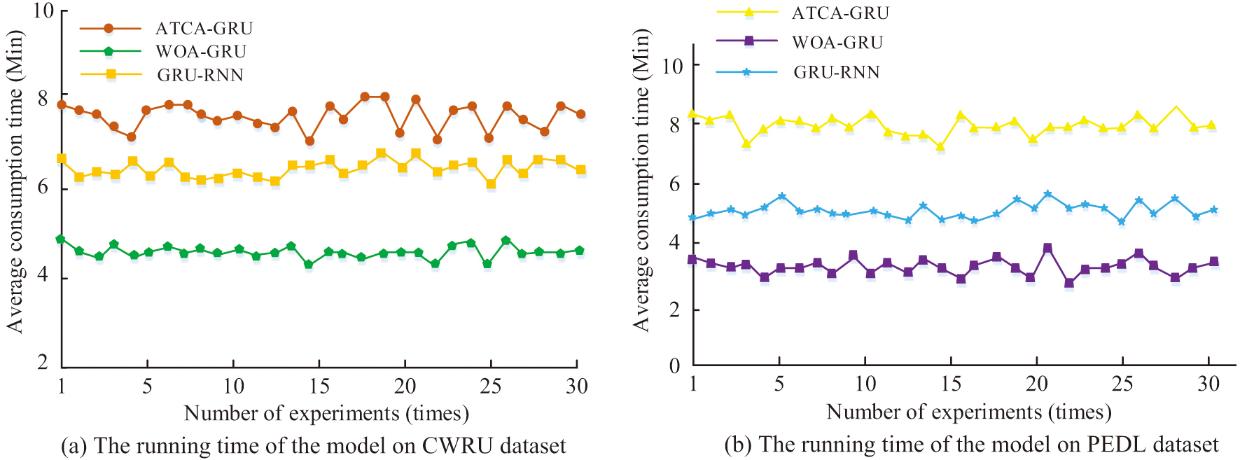Fig. 12. Comparison of running times of different models.

To verify the real-time effectiveness of the proposed model for CPFP, the study takes the in-use CP atlas as an input and the output is shown in Fig. 13. In Fig. 13, the model marks the points that may have hidden faults, which makes it easy for the maintenance personnel to overhaul the CP.

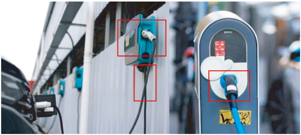Fig. 13. WOA-GRU model outputs fault prediction points.

The model suggested in this study performs well in all performances and has certain benefits over other models of the same type, indicating that it is an advanced model based on the aforementioned experimental results.

V.CONCLUSION

The world’s NEV market has rapidly grown and now holds a significant market share. The rise of NEVs presents new opportunities for the automobile industry and demands new infrastructure. Specifically, the construction and development of CP has become a key focus. In this context, the emphasis on CP should match the market position of NEVs to meet the growing demand for NEV charging. Aiming at the CPFP problem of NEVs, this study designed a fault judgment model that incorporated the GRU and WOA. Based on the model performance test experiments, the WOA-GRU model achieved an average prediction accuracy of 92.02%, with an average recall of 85.66% and an F1 value of 93.87%. The WOA-GRU model also demonstrated a significantly lower average running time on the CWRU and PEDL datasets compared to other experimental models. Additionally, the proposed model exhibited larger areas under the ROC curves and reference lines compared to the control model. The experimental results validated the progress of the suggested model in this work by showing that it performed better than the control model in terms of F1 value, recall, and prediction accuracy. However, the study also found overfitting of the proposed model, which was caused by the fast convergence of the GRU network. Subsequent studies can further improve the proposed model to construct a better CPFP model.

Charging Pile Fault Prediction Model Based on GRU Network and WOA