JAIT

I.INTRODUCTION

Robotic navigation is a relevant topic in a world where autonomous navigation systems are starting to get implemented and could be useful in industries like automotive, logistics, and industrial management. New methods in autonomous navigation could aid in automation of many tasks as well as creating efficiencies in several industries. On the other hand, these systems so far have proven unreliable when it comes to success rate and performance, which leads to them not being useful enough to be implemented. Therefore, it is important to find new methods and refine existing ones.

One way to divide robotic navigation is into motion and navigation. Thus, some researchers have been done in the motion field to make the robot movement “smoother,” for example, using Bezier curves and other geometric features [1–4]. On the navigation front, the most common method is using ultrasonic sensors to measure distances as an input to a control scheme, frequently fuzzy logic, or a geometric inference as in [5–10]. In recent years, Light Detection And Ranging (LiDAR) has become common alternative to ultrasonic sensors [11,12]. These have been popularized because they provide relatively accurate distance information of their environment with simple processing, but with its high cost of as main disadvantage. Furthermore, there is currently great interest in the use of vision systems as the main input for navigation. Thus, RGB-D has been employed because it provides images that can be used for object identification and still provide depth information similar to the ultrasonic sensors and LiDAR [9,10,13,14]. However, these approaches rely on having a dedicated sensor to perceive depth and not purely on vision. The most common purely vision-based method for navigation is the use of multi-camera arrays which use techniques such as stereoscopy to estimate depth [15–19]. On the other hand, another less common method is through the use of structured light like the Kinect sensor [20]. Finally, there is the monocular vision methods, which are challenging since there are no other sensors involved to aid in-depth estimation. Therefore, these use other algorithmic solutions to address the navigation problem [21–24]. In this paper, we will be exploring the use of monocular vision in conjunction with fuzzy Q-learning (FQL) for robotic navigation in an unknown environment. On the one hand, FQL is a rules-based control approach for mobile robots with ultrasonic sensors or cameras [25–31]. On the other hand, instead of estimating depth we will use an optical flow estimation technique as was proposed in [32]. This technique estimates the amount of movement in each pixel between two images which can be processed to calculate a direction without obstacles. The advantage of this type of system is that it does not require previous knowledge of its environment and it does not require mapping to navigate unlike the LiDAR or ultrasonic sensor approaches. In addition, we improved the FQL approach reported in [31] by adjusting the reinforcement signal. This signal comes from the measurement of optical flow density in an area recorded by the camera and determines whether that region is considered “dense” or “thin,” and through the addition evolutionary component, which involves time-series measures from various ultrasonic sensors on the current and previous execution loops with the objective of helping it continue learning when its performance stagnates. Finally, the proposed system was implemented and tested in a virtual robotics environment.

The remainder of the paper is organized as follows: in Section II, the virtual robotics environment, the FQL approach, and the optical flow method used are presented. Section III shows the proposed vision and FQL-based autonomous navigation method. Experiments results of control to obstacle avoidance are reported in Section IV. Finally, the discussion and conclusions are given in Sections V and VI, respectively.

II.MATERIALS AND METHODS

A.COPPELIASIM SIMULATION ENVIRONMENT

CoppeliaSim is a simulation environment for robotics dynamics and control testing. The simulation environment can be modified to create multiple testing scenarios and be able to test the control systems and dynamics of robots and to track their trajectories. In this paper, we use the CoppeliaSim Edu version [33].

To test the proposed navigation autonomous control, we use the Pioneer P3-DX as our surrogate robot (Fig. 1a). Pioneer P3-DX robot is a two-wheel and two-motor differential drive robot, which includes ultrasonic sensors to measure distances to obstacles. In addition, we added an RGB camera with a resolution of 256 × 256 pixels and a field of view of 60°.

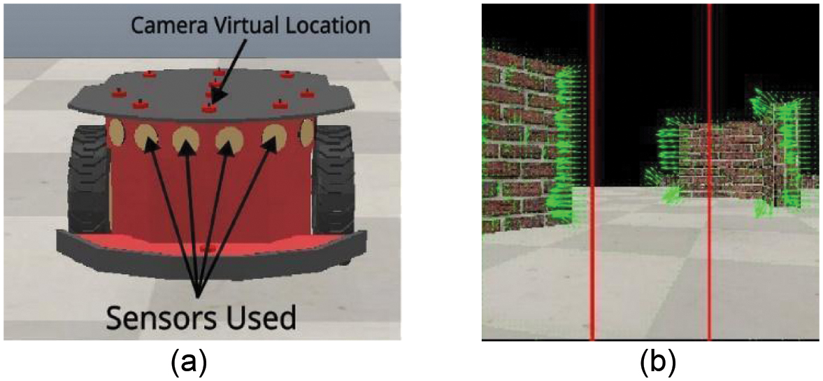Fig. 1. (a) P3-DX robot. (b) Optical flow vectors between two consecutive images.

The simulation environment of CoppeliaSim is configured to run on real time in a Ryzen 7750x up to 5.5 GHz CPU with 64 GB of RAM. It is also tested in an i7-10750H up to 2.8 GHz CPU and 16 GB of RAM and did not use all system resources. Therefore, the simulation can be done in lower capacity equipment.

B.OPTICAL FLOW ESTIMATION METHOD

The optical flow methods estimate the spatial displacement between the pixels of two consecutive images. These displacements generally are associated with intensity variations of local structures in the image sequence [32] and generally a larger optical flow indicates objects that are closer in proximity to the camera since they would shift more pixels. This is estimated by assuming that the change between images in time will be close to zero. The optical flow constraint equation holds that E_xu + E_yv + E_t = 0, where E = E(x,y,t) relates to the intensity of the image in the spatial coordinates x,y and time t, E_* is the derivative of E with respect to *, and u and v are the displacements from a time t to a time t + 1. Due to this equation having two unknown variables, a constraint is needed to approximate the rate of change, and in [32], the smoothness constraint is proposed as shown in (1):

\int \int [α^{2} (| {| \nabla u | |}^{2} + {| | \nabla v | |}^{2}) + (E_{x} u + E_{y} v + E_{t})] d x d y = 0,

(1)

where α is a weighting factor which aids in areas where the brightness gradient is small and ∇² indicates the Laplacian [32]. The result of solving (1) are the motion vectors (u,v)^⊤ for each pixel which represent the perceived movement between two consecutive images as shown in Fig. 1b.

Optical flow, however, has some limitations due to it using assumptions to be able to calculate the optical flow. One of these assumptions is that the movements between images are slow. Therefore, if there are sudden movements or the robot moves too fast, it can lead to some inaccuracies. However, it allows for a simple model to be implemented in real time. On this work, this method was selected due to ease of implementation and due to its novelty as unlike most other methods. It does not require measuring distances in its environment.

C.FUZZY Q-LEARNING

FQL is a combination of fuzzy logic and Q-learning, where the fuzzy portion defines the rules and takes actions based on the states of the system [25,26], while the Q-Learning is in charge of generating a reward which alters the functions of the inference made by the fuzzy logic portion to make it adapt to new situations. These rewards are based on another set of functions and rules that define them. Thus, the system over time “learns” by estimating the discounted future rewards given the actions performed from states. The Q function value estimation equation is shown in (2) [27]:

Q (S_{t}, A_{t}) \leftarrow Q (S_{t}, A_{t}) + ε [R_{t + 1} + γ \underset{a}{m a x} Q (S_{t + 1}, a) - Q (S_{t}, A_{t})],

(2)

where S_t is the current state, A_t is the action in S_t, Q(S_t,At) is the estimated sum of discounted reward carried out by an action A given a state S, ε is the learning rate, γ is the discounting factor, S_(t+1) is next state, R_(t+1) is the reward in the new state, and a is the action with the largest q-value in a given S_t.

III.VISION-FQL-BASED OBSTACLE AVOIDANCE CONTROL

A.CONTROL SCHEME

Figure 2 shows the overall schema of the obstacle avoidance control based on vision. It uses the optical flow method described in Section II.B as input and a closed-loop FQL controller described in Section II.C.

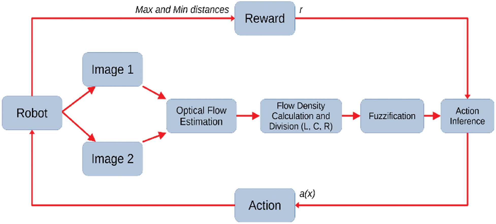Fig. 2. Obstacle avoidance control overview.

The inputs for the proposed obstacle avoidance system consist of motion densities. These densities were obtained from the optical flow estimation through three horizontal areas of the images (R_i+n) corresponding to left ( $n = 0)$ , center ( $n = 1)$ , and right ( $n = 2)$ areas of the images as it is shown in Fig. 1b. Then, they were fuzzified into “dense” and “thin” fuzzy sets, dense meaning that there is more perceived moment and thin the contrary [31]. The procedure to calculate these densities is described in (3):

\underline{R_{i}} = \frac{\underline{R_{i}}}{m a x {\underline{R_{i}}, \underset{¯---}{R_{i + 1}}, \underset{¯---}{R_{i + 2}}}},

(3)

where

\underline{R_{i}}

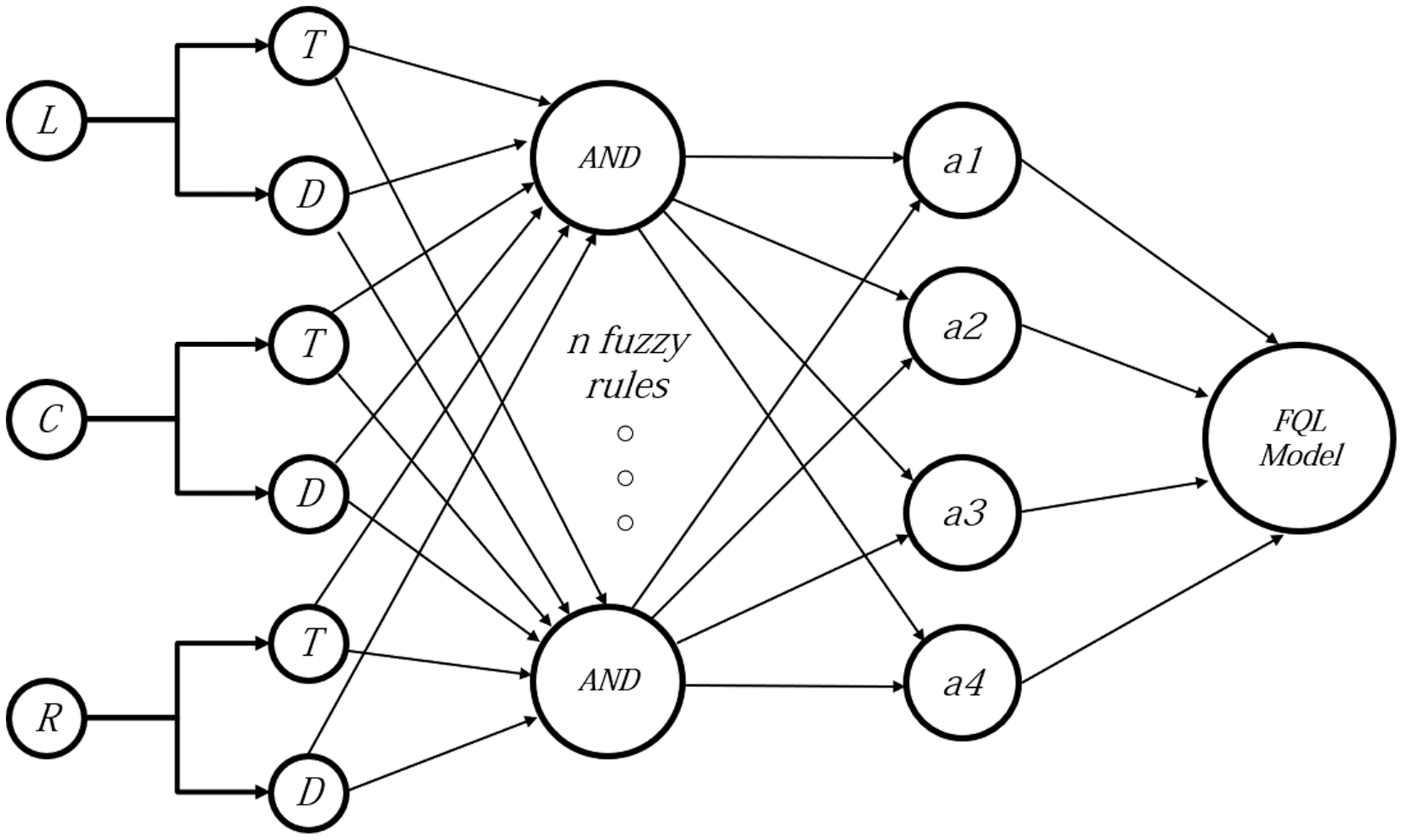
are the normalized magnitudes of each region (left, center, and right) with respect to the area with the maximum average registered. The fuzzy input membership functions have been changed from the ones used in [31] to the ones shown in Fig. 3. To determine the state of the robot, the three fuzzified inputs are compared to one of eight states or rules (Ru) in Table I, which are the different combinations of “thin” and “dense” (T or D) for R_i+n sections; in turn, these states can take one of four actions a1, a2, a3, and a4 which correspond to going forward, left, right, and back and then turning right. The proposed FQL architecture is shown in Fig. 4, where the fuzzy system used operates with eight fuzzy rules, whose inputs are the densities mentioned in (3) as knowledge base, and as it is shown in Table I, where | represents logical OR and max represents the maximum q value present on a given row of a fuzzy rule. The q values with which the actions are selected change over time through the reward function or reinforcement signal and an error signal. For this application we propose a reinforcement signal that measures the distance to the objects using the four central ultrasonic sensors of the P3-DX robot (Fig. 1a). These will provide rewards in real time depending on whether the robot is getting closer or farther to a collision and the space it has to maneuver so it registers the maximum distances from the ultrasonic sensors, if the sensors do not detect anything the distance defaults to 999. This is designed to consider the maximum and minimum distances read by the sensors.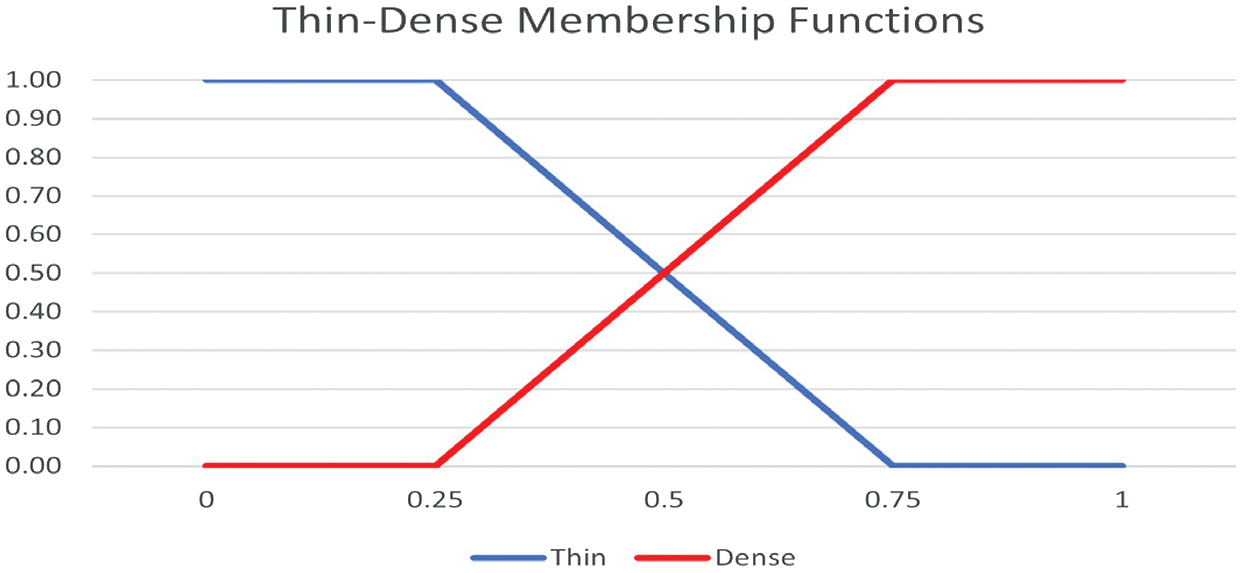

Fig. 3. Input membership functions.

Table I. Fuzzy rules implemented in the controller

Ru	R_i	R_i+1	R_i+2	Action	q(i,j)
1	T	T	T	a1\|a2\|a3\|a4	mx q1,j
2	T	T	D	a1\|a2\|a3\|a4	mx q2,j
3	T	D	T	a1\|a2\|a3\|a4	mx q3,j
4	T	D	D	a1\|a2\|a3\|a4	mx q4,j
5	D	T	T	a1\|a2\|a3\|a4	mx q5,j
6	D	T	D	a1\|a2\|a3\|a4	mx q6,j
7	D	D	T	a1\|a2\|a3\|a4	mx q7,j
8	D	D	D	a1\|a2\|a3\|a4	mx q8,j

Fig. 4. FQL architecture.

The reward system is shown in Table II, where the distance obtained from the ultrasonic sensors is considered. In this manner, the minimum distance registered by the sensors d_min is compared to define the reward value. Thus, dl = 0.14 is the collision threshold distance when a sensor registers a distance lesser than d_l, the algorithm enters into the first condition shown in Table II, and therefore the robot gets a fixed negative reward signal and the simulation ends. pd_min is the distance registered by the sensors on the previous execution loop, dt is the distance to the target, pdt is the distance to target (circle green in the scenarios shown in Fig. 7) on the previous execution loop, d_max is the maximum distance registered by the sensors, and α = 1 × 10⁻⁵.

Table II. Fuzzy rules implemented in the controller

Condition	Reward function
d_min≤ d_l	–2α
d_min ≥ pd_minor d_min≥999	$α + α (\frac{pdt - dt}{dt})$
d_min≤ pd_min	$- α (\frac{d_{\max}}{d_{\min}}) + α (\frac{pdt - dt}{dt})$

The idea of considering d_min and pd_min as conditions is to “reward” when the robot gets farther from an obstacle and therefore enters into the second condition and to “punish” the robot when it gets closer to an obstacle and enters into the third condition, and d_max is used to moderate the reward signal when it is a “punishment” by considering how much distance it has to maneuver. Finally, the logic behind using pdt and dt as inputs is to direct the robot toward the target. It is used in the second and third conditions to modify slightly the reward by taking into account how much it approached the target regardless of being closer or farther from an obstacle, and the rewards associated with getting closer to the target are approximately an order of magnitude lower, so the robot prioritizes avoiding collision, but still gets “rewarded” for getting closer to the target and “punished” when getting farther from it.

The error signal is calculated through the quality value V(x,a) and the calculated q value Q(S_t,A) using (4) [12]:

Δ Q = r + γ V (x, a) - Q (x, a),

(4)

where

r

is the calculated reward and

γ

is a discount factor. With that error signal the new

q

value, for the action taken, is updated as it is shown in (5):

(i, j^{0}) = q (i, j^{0}) + Δ q (i, j^{0}),

(5)

where q(i,j⁰) is the q value of the action taken, and the value of Δq(i,j⁰) can be obtained through (6):

Δ q (i, j^{0}) = ε \times Δ Q (i, j^{0}) \times \frac{a_{i} (x)}{Σ_{i = 1}^{N} a_{i} (x)},

(6)

where ε is a discount factor, and for our tests it was fixed to 0.2.

The behavior of the reward function depends on the corresponding condition of Table II; for the first condition, the value of the reward function is fixed, for the second condition, where the robot is rewarded, and the behavior is linear as shown in Fig. 5. The third condition depends mostly on the relation between d_max and d_min, maintaining a constant d_min, pdt, and dt, and its behavior is linear as shown in Fig. 6 (red plot). However, when d_max is constant instead of d_min, its behavior becomes of the form $- \frac{n}{x}$ as shown in Fig. 6 (blue plot).

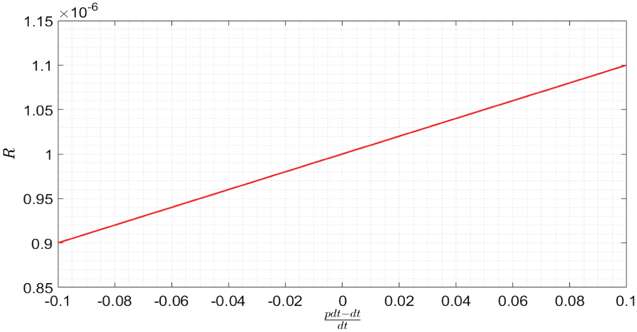Fig. 5. Reward response on condition 2.

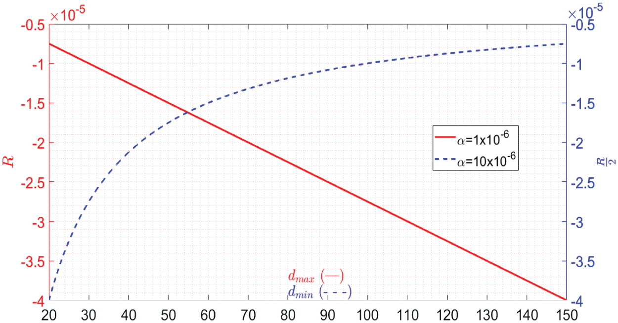Fig. 6. Reward response on condition 3. With fixed dmin (red plot) and with fixed dmax (blue plot).

Compared to the method explored in [31], the reinforcement signal proposed on this paper is able to judge not only if the robot has collided or not but also how well it is navigating based on the reward responses shown in (5) and (6) providing a proportional signal instead of a fixed reward.

B.EVOLUTIONARY CORRECTION

In the experiments carried out, it is observed that after certain number of iterations, the system tends to stop improving. Therefore, we implemented an evolutionary system based on conditions, so in the case that the system’s performance during training decreases it can use existing Q tables from previous iterations, distinguish the ones which had the best performances, and combine and mutate them, so it can better retain previous knowledge.

The method implemented is a genetic algorithm, where the “parents” are the three best Q-tables, whose score is based on the minimum distance reached to a set target in the scenario, and the “child” is the average of the parents, where each element of the resulting “child” Q-table is mutated according to (7), where R_rand is the mutation matrix where each cell contains a random value within the range of 0.95 and 1.05:

\frac{Q_{t a b l e 1} + Q_{t a b l e 2} + Q_{t a b l e 3}}{3} \times R_{r a n d},

(7)

where Q_tablei, with i = 1,…3, are the three best-performing models at the end of the iteration.

IV.TESTING AND RESULTS

In this section, we show the tests performed to evaluate the proposed vision-FQL-based obstacle avoidance control and compare them to the one proposed in [31]. The main differences between the proposed method and that reported in [31] correspond to the reward function as shown in Table II and the evolutionary behavior reported in (7).

For testing, we used three scenarios defined in the CoppeliaSim environment as shown in Fig. 7. The scene in scenario 1 consists of a curved path, Scenario 2 is a curved path with two consecutive turns, and scenario 3 which is an open maze. For scenarios 1 and 2, we placed a target at the end of their paths and in scenario 3 we placed it on an arbitrary location, and the targets are located in the green circles of Fig. 7. The targets have two purposes, to end the simulation if the robot reaches it and start a new iteration, and its location is used to calculate the distance between it and the robot to provide the feedback for the evolutionary system proposed in Section III. Three experiments are performed. The first experiment is to compare the ability of the response system and evolutionary methods proposed in Sections II.C and III.B to the ones proposed in [31] to reach the targets of each scenario, the second test will evaluate their ability to find multiple solutions to the same scenario, and the third will evaluate whether or not it is effective to train the robot in one scenario with a model from another scenario as a starting point. Because scenario 3 is the most complex, the successful attempt will be the first attempt to get within 10% of the distance to the target.

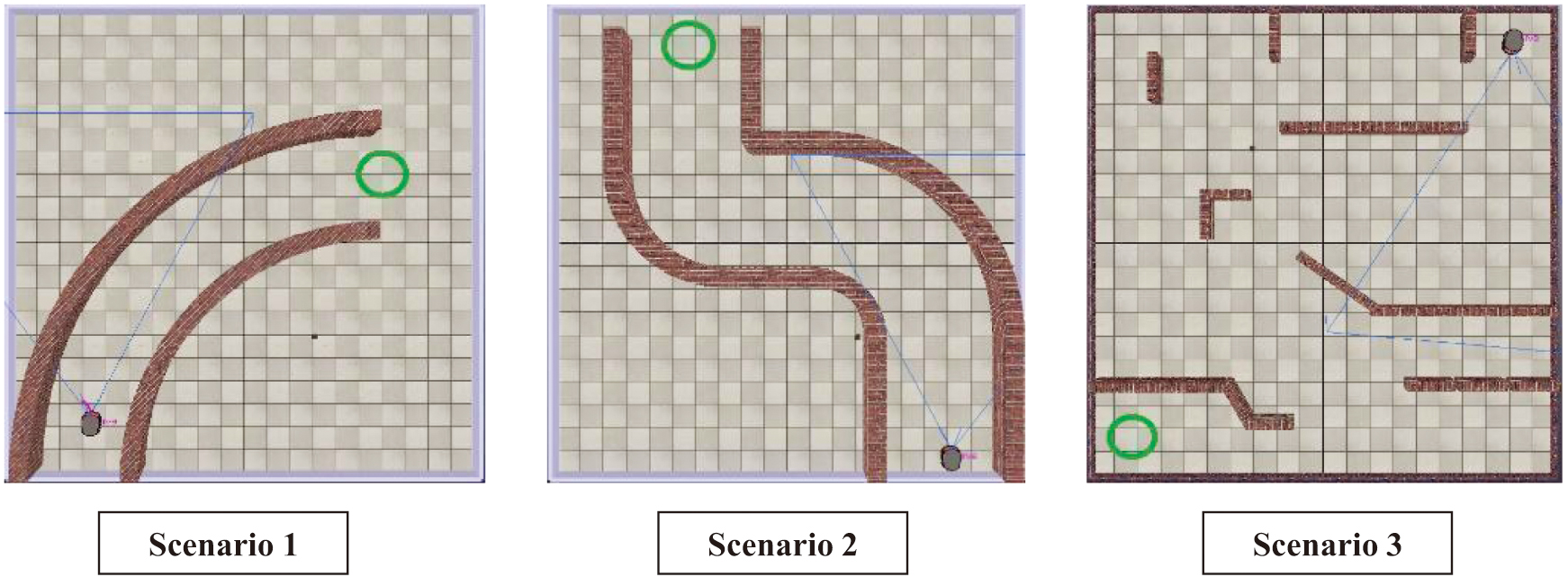Fig. 7. Testing scenarios defined in the CoppeliaSim environment.

In Tables III and IV, we report the results obtained after performing the three experiments, where R0 corresponds to the response system proposed in [31], R1 corresponds to the response system proposed in Section III.C, and “non evo” and “evo” designations indicate if that algorithm used the evolutionary correction mentioned in Section III.B.

Table III. Results for experiment 1: attempts to reach a solution

Model	Scenario 1	Scenario 2	Scenario 3
R0 non evo	5	14	N/A
R1 non evo	1	5	N/A
R0 evo	2	28	15
R1 evo	1	12	N/A

Table IV. Results for experiment 2: ability to continue learning

Model	Scenario 1	Scenario 2	Scenario 3
R0 non evo	4	3	0
R1 non evo	3	2	0
R0 evo	7	3	3
R1 evo	7	3	0

Table III shows the results for experiment 1, reporting the amount of attempts it took each algorithm variant to reach the target in each scenario.

From Table III, we can see that the proposed response system tends to reach a solution in a lower number of attempts than the one proposed in [31]. However, the evolutionary version of the original response system was the only one to get within 10% of the distance in the third scenario. Figure 8 shows some successful attempts.

Fig. 8. Examples of solutions reached by the algorithms, in scenario 1 and 2 by R1 evolutionary algorithm and for scenario 3 the R0 evolutionary algorithm.

The second experiment focused on the ability of the models to learn multiple solutions to the scenarios, and for the case of the third scenario we will only consider those that reached within 10% of the initial distance since none were able to reach the target. Thus, Table IV shows how many solutions were reached by each algorithm.

From Table IV, we can see that the evolutionary models show greater ability to learn multiple solutions than the non-evolutionary approaches.

The last experiment is done to determine if it is better to train the model from another model trained in another scenario; in this case, we used the previous scenario (e.g., a model trained in scenario 1 used in scenario 2) and the R1 response system, and the results are shown in Table V.

Table V. Results for experiment 4: attempts to reach a solution from a model trained in a previous scenario

Model	Scenario 1 to 2	Scenario 2 to 3
R1 non evo	12	N/A
R1 evo	46	N/A

Table V shows that it took a larger number of attempts than the regular starting point to reach a solution to scenario 2, significantly reducing its performance and did not reach a solution for scenario 3. Therefore, there is no evidence that starting from a model trained in another scenario improves training, and this may be due to the scenarios not being similar enough to benefit the training of the models.

V.DISCUSSION

In general, the proposed response system tends to get to a solution in a lesser number of attempts than the one proposed in [31]. Although the results are mixed, the evolutionary correction tends to help the system in finding more possible solutions. Starting the training using a model trained in another scenario does not reduce the number of iterations it takes to find a solution.

Implementation is relatively straightforward; however, there are some issues especially with the simulation environment. There is some variability on the behavior of the simulation depending on which system runs it. CoppeliaSim struggles with imported models. Therefore, we limited the complexity of the environments. Also, CoppeliaSim is not as widely used as some other programs, and there is a lack of resources to consult on how to implement features, limiting the variety of experiments and environments we could test. Finally, the simulator does not work natively with Python and has to be implemented through the use of an API. Therefore, we think that it may be beneficial to use a game engine such as Unity or Godot which would allow for more flexibility and have more resources with the disadvantage that the algorithm would have to be translated to another programming language and create new simulation scenes.

The results obtained showed that the reinforced learning, with a vision-based control strategy and an evolutionary reward signal, improves the traditional FQL strategy by taking into account the time behavior of the robot. These findings are relevant to develop new applications where the continuous learning of the robot is a critical factor, for example, autonomous vehicles that use low-cost and real-time vision-based methods instead of computationally expensive ones such as LiDAR-based methods. On the other hand, it is observed that with the current optical flow system, the robot can struggle with change of direction due to new objects appearing on its visual field, when a new object appears the area in which it appears is considered “dense” and overshoots the response as shown in Fig. 9(a). This overshoot tends to get the robot in a situation where it is facing directly against a wall where the flow density tends to be low and therefore does not identify it as an obstacle and eventually collides. Another identified failure mode is related to the angle of view of the robot; in some iterations, the robot initially avoids the obstacle. However, the 60° field of view of the camera is sometimes insufficient to detect objects that are near and to the side of the robot and therefore navigates too close to an obstacle as shown in Fig. 9(b).

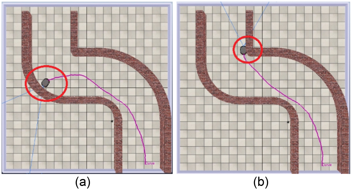Fig. 9. Identified failure modes. (a) Appearance of new objects. (b) Objects not detected given the viewing angle.

To address these issues, there are two proposals: the first would be to add more regions to the optical flow and therefore the rules of the fuzzy controller, and five regions instead of three would allow for a more precise control and prevent overshooting when a new obstacle is detected. The second proposal is increasing the field of view of the camera to prevent the second identified failure mode, and another proposal is a hybrid approach in which the ultrasonic sensors are used to determine a state in which the robot is too close to an obstacle and does a routine to get the robot in a state where it can continue its navigation using the camera. This would help in both identified failure modes. It would also be possible to use the optical flow as input for another machine learning model such as primal policy optimization.

VI.CONCLUSIONS

In this paper, an FQL and optical flow-based autonomous navigation approach was presented. The proposed method incorporated a new reward system including the ultrasonic sensors and an evolutionary component which enables it to keep learning indefinitely without having prior knowledge of its environment or mapping. The results obtained show that the present approach improves the rate of learning compared with a method with a simple reward system and without the evolutionary component. The findings show that the proposal enables us to test more solutions and help us find a model better suited to the scenario it is trained on, allowing the robot to navigate using only one camera while keeping the model relatively light on processing resources.

In future work, we will explore adding more regions to the optical flow and to modify the architecture of the fuzzy system or using a different algorithm such as primal policy optimization. Also, we will incorporate a hybrid approach using the ultrasonic sensors to determine a state in which the robot is too close to an obstacle. In addition, we will consider changing the simulation platform, for example, Unity and Godot are popular alternatives due to abundance of documentation, large community, and flexibility.

A Vision-based Robotic Navigation Method Using an Evolutionary and Fuzzy Q-Learning Approach