I.INTRODUCTION
One of the most fatal ailments is cancer that strikes people nowadays and poses a threat to their lives. The World Health Organization predicts that by 2020, cancer will be the biggest cause of death globally [1]. Lung cancer is thought to be responsible for the 1.80 million cancer-related fatalities worldwide. Considering projections, cancer would be responsible for 60% of mortality by 2035 [2]. Lung tumors are made up of large numbers of lung cells that have undergone an uncontrolled change. The prevalence of lung cancer has increased globally due to a number of factors. Inhaling hazardous or dangerous substances, which affects a significant number of the senior population in society, is one of the reasons. Smoking cigarettes increases the risk of lung cancer in men by 90% and in women by 70% to 80% [3]. Even those who have never smoked are at danger of developing lung cancer. The most typical lung cancer subtypes are adenocarcinomas and squamous cell carcinomas. Additionally, there are the histological subtypes of small- and large-cell carcinoma. Treatment is more challenging, though, because lung cancers, both big and small cell, can arise in any part of the lung they have a tendency to spread rapidly [4].
When aberrant lung cells multiply uncontrollably and develop into a tumor, squamous cell carcinoma results. One organ where cancer cells can spread (metastasize) is the lymphatic vessels, which are found around the lungs, liver, adrenal glands, bones, and brain. If left undetected, the condition may develop into squamous cell carcinoma [5]. The incidence and death rates of lung cancer are among the highest of any major cancers in the world as a result. Early identification and therapy of lung cancer are crucial to identification of suspicious lung nodules [6]. The physical characteristics of the malignant cells include an unusually shaped and enlarged nucleus [7]. It is common practice to use the morphological features of computer tomography (CT) scans to differentiate between healthy and unhealthy nodules. Another approach is tried by training the classifiers to detect whether the tissue is cancerous or not. There are other methods that may be applied, including single classifiers and classifiers that combine multiple characteristics [8]. Identifying potential malignant lung nodules is essential for obtaining a lung cancer diagnosis. Lung cancer can be distinguished from benign nodules by contrasting their features [9]. For an appropriate nodule evaluation, careful examination of the morphologic features is necessary because There is significant overlap between the traits of nodules that are both benign and malignant. Additionally, morphological analysis is necessary for early diagnosis [10].
The identification, segmentation, and categorization of benign and malignant nodules in the lungs are the key research areas for the application of imaging techniques based on deep learning. To enhance the functionality of deep learning models, research mostly focuses on creating novel designs for networks and loss functions. Recent reviews of deep learning approaches have been published by a number of research organizations [11–13]. However, deep learning techniques have advanced quickly, and a number of fresh ways and uses appear every year. The study’s remaining sections are structured using shadows: The relevant works are summarized in Section II, the suggested model is briefly explained in Section III, the findings and validation analysis are shown in Section IV, and the summary and conclusion are given in Section V.
II.RELATED WORKS
In their work, Li, X., et al. [14] imaginatively proposed a Bidirectional Pyramid component and a Cross-Transformer module to successfully circumvent the aforementioned two shortcomings, by merging its self-awareness on the inside and outside. The latter minimizes feature inconsistencies at various stages of the model by incorporating bidirectional entry points into the characteristic pyramid that are used to encourage feature information exchange between the shallow and deeper layers of the model. A comprehensive lung nodule analysis significantly improves overall performances such as Dice Similarity Coefficient and sensitivity. The model put forward in this research has exceptional lung nodule segmentation performance, and it can assess the size, form, and other characteristics of lung nodules, which is very useful for clinicians in the early identification of lung nodules and has tremendous clinical importance.
In their paper, Annavarapu, C.S.R. et al. [15] created a resource-effective end-to-end deep learning method for segmenting lung nodules. Between an encoder and a decoder, a bidirectional feature network is used. To increase the effectiveness of the segmentation, it also makes use of the Mish function of activation and the class strengths of masks. Using the 1186 lung nodules in the publicly available LUNA-16 dataset, the suggested model was thoroughly tested and trained. The network training parameter was each training sample’s weighted binary cross-entropy loss to increase the probability that each voxel in the mask belongs to the correct class. Additionally, the suggested model’s robustness was assessed using data from the QIN Lung CT project. The evaluation compares the performance of competing deep learning models and provides the U-Net as better than other deep learning models.
The study of Mothkur, R., and Veerappa, B.N. [16] set out to evaluate various deep learning architectures for image processing that are memory-efficient and portable. With an accuracy of 85.21 percent, the suggested compact deep neural network outperforms by making an appropriate trade-off between specificity and sensitivity. The proposed study employs binary classification networks to distinguish between lung cancer in its early stages and other types of cancer in patient CT pictures. These networks include 2D SqueezeNet, 2D MobileNet, and plain old 2D CNN.
Tyagi, S., et al. [17] devised a technique for segmenting lung tumors that combines the convolutional neural network and the vision transformer. Convolution blocks are employed in the earliest layers of the encoder and the decoder’s last layers, which capture features that communicate the most crucial information. This network is designed as an encoder-decoder structure. Transformator blocks with self-attention mechanisms are used in the deeper layers to produce more precise global feature maps. For network optimization, they make use of a recently proposed unified loss equation that includes dice-based and cross-entropy losses. After training it using an NSCLC-Radiomics dataset that is accessible to the public, they evaluated the generalizability of their network using a dataset they obtained from a neighboring hospital. The results are based on the average Dice coefficient and average hausdorff distance for each method, respectively.
Techniques like enhanced backpropagation of feed-forward neural network (EBFNN), convolution neural network (CNN), and random forest (RF) were used by Wahengbam and Sriram [18] in their investigation. When these algorithms’ accuracy was evaluated, it was discovered that EBFNN outperformed other methods. The four essential processes in the execution of the suggested model are preprocessing, segmentation, feature elimination, and classification. Utilizing a common set of images gathered by the Lung Image Database Consortium (LIDC), the implementation step’s results are reviewed from a number of angles. The results show that, compared to RF accuracy levels of 89% and CNN accuracy levels of 91%, the recommended EBFNN provides accuracy levels of about 93%.
Using both whale optimization and bacterial foraging optimization, Alameen, A.'s study [19] aimed to create a fused evolutionary technique that enhances feature extraction. For the classification process, a dual-graph artificial neural network (CNN) was employed. The study evaluate the fused model’s performance using several metrics and methods. Initially, the input CT image is used to determine whether the lesion is malignant or not. A number of methods, including the Histogram-oriented gradient features, gray-level co-occurrence matrix, and Gray-level dependency matrix, are applied to the pre-processed segmented picture to extract its geometrical, statistical, structural, and texture features. The best features should be chosen using a brand-new fusion method called Whale-Bacterial Foraging Optimization. Lung cancer classification has been carried out using dual-graph convolutional neural networks. Algorithms for classification and optimization have been compared in study.
III.PROPOSED METHODOLOGY
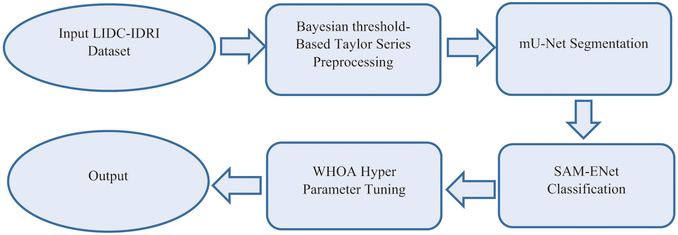
Figure 1 represents the pipeline of the proposed work.
A.DATASET DESCRIPTION
The LIDC-IDRI dataset was used to create the suggested model [20], which has 1012 variable-slice-thickness LDCT scans. Diameter-specific nodules were verified to confirm whether they were actual nodules. The collection also includes a numerical description of a number of nodular traits. Specifically, the transparency of the nodules is indicated by the nodule texture, where 1 denotes an entirely solid nodule and five entirely non-solid nodules. 2 284 nodules were evaluated from the 888 images used for the LUNA16 challenge 18 (due to irregular annotations, inadequate scan reconstruction, or high slice thickness, several samples were discarded). Of those, 1 593, 1 190, and 790 had a level 2, level 3, and level 4 of agreement. Nodules are classified as sub-solid in our testing if its average consistency is lower than 5, solid in our tests if it is more than 5, and non-solid in all other cases. There are 1695 solid nodules in the dataset, with a common agreement level of 2, 300 sub-solid nodules, and 135 non-solid nodules [21].
The average center of masses of the specialized annotations served as the patching point for all nodules, which were subsequently isotopically scaled to 64 × 64 × 64 voxels. Volume picture intensity was linearly transformed from [400, 1000] to [0, 1] Hounsfield Units. The optimizer Wildebeest Herd Optimization Algorithm (WHOA) was employed (learning rate 0.001), and an 8-sample batch size was employed to train the network. To accommodate for inter-observer variability, all agreement levels were taken into account; nonetheless, the algorithm was trained by matching the same nodule with a number of reliable ground truths. Additionally, this paper used 20% of the training for validation and evaluated proposed model using stratified five-fold cross-validation using scan-level partitions. Using 100 search steps and a random search20, all hyper-parameters were located. At each step, , where U is a uniform distribution. The initial train-test split’s validation set was subjected to optimization.
B.PREPROCESSING
The first step in denoising lung pictures is to enhance their quality [22]. The Bayesian threshold-based Taylor series strategy is suggested in this study as a method for turning noisy pixels into pixels of higher quality. Since the Taylor series offers high-resolution wavelet subbands, this suggested method is based on it. An infinite number of terms resulting from derivatives are defined by the Taylor series with pixel-based and changeable values. A 3D frame is required for the Taylor series as equation (1).
Since an image’s intensities are not uniform throughout, images typically have a variety of pixel values. For denoising, the variations in pixel values therefore require greater consideration. The noise in subbands is calculated from the defined Taylor series and removed if it exceeds the predicted Bayesian threshold. The following equation (2) is used to calculate the threshold for all subbands:
where indicates the assessment of the noise, and the threshold was reached for all bands.When , It is written as equation (3).
where is defined as equation (4).The subbands are . This is regarded as the overall number of subbands, and is influenced by equation (5).
After calculating the following an arrangement of the acquired Bayesian threshold values, an expression is created by applying the curve fitting technique by equation (6):
In Equation (6), provides a definition of the standard deviation of the noise and the amounts of other variables such as , , , and . The mathematical formulation of the BM3D filtering technique is then used as equation (7):
In Equation (7), the T3D is defined as single 3D transform. Each subband is reconfigured and achieves denoised frames from this final formulation. The process of intensity normalization, which follows, is carried out with a range between 0 and 1. Intensity normalization uses the Z score normalization function, whose performance is superior to that of the decimal and min-max normalization methods. The following is how this normalization function is calculated:
Where represents the voxel intensity at location k, variance as δ and intensity’s mean value as μ. When preparing an image for subsequent processing, the rational range (0–1) was employed for intensity normalization using the Z score normalization tool. For operations involving training and testing, this phase is required for all photos.C.mU-NET SEGMENTATION
To avoid repeating low-resolution feature map data, the network that is suggested uses a residual path. After pooling in the potential network, the remaining route is positioned to the right, as seen in Figs. 2(b)–(d), in contrast to the prior study from [23]. After pooling, the remaining layers are placed to right side position and it is shown in Figs. 2(b)–(d), which is contrasted from the previous study [23]. This adaptive filter’s performance was evaluated using a predetermined permeation rate as equation (9):
where a is the residual path being followed by the normalized feature map in the skip connection. , where each label represents the binary mask of the item (lung or lung tumor) and x, y presents the residual path and a standardized feature map. The range of each normalized feature map is [0, 1]. The penetration rate was set to –0.5 when . This means that the skip connection lacks any useful functionality.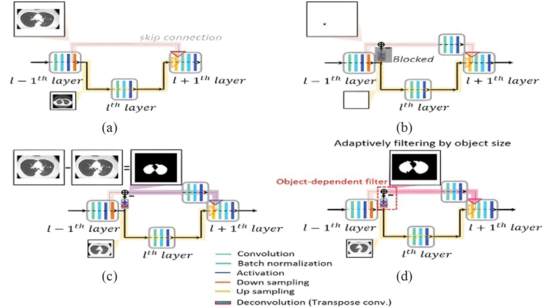 Fig. 2. Diagram showing the proposed mU-Nets in (b) and (d) and the standard U-Net in (a). (a) When using a traditional U-Net, all feature information travels only low-resolution data transmitted to the next level via the skip link. Small objects’ spatial information frequently vanishes after pooling owing to resolution loss. (b) For small objects in the mU-Net case, pooling allows for the extraction of higher-level global characteristics without sacrificing resolution. Small object characteristics can enter the connection that skips without being deleted by pooling because the deconvolution path is blocked, preserving the location data of small objects. (c) To prevent the repetition of low-resolution information, feature information for large objects in the mU-Net example is limited to edge information in the skip connection. (d) The suggested network is represented schematically. Depending on the size of the item, deconvolution and activation in the residual path merge leftover path elements into skip connection features.
Because pooling destroys spatial information, as illustrated in Fig. 2(b), a few pooling layers may be sufficient to extract the small object’s overall features. Less information is wasted due to pooling as seen in Fig. 3, which results in more effective feature extraction for small objects. As illustrated in Fig. 2(b), the residue path is used to preserve tiny object information and subsequent convolution layers to the bypass connections to extract greater-level features. This adjustment allows penetration rates of minor object features to remain high at early stages while preserving information that would be lost following additional poolings, as illustrated in Fig. 3. As the stage grows, information on little objects eventually disappears, as seen in Fig. 3 with penetration rates of –0.5. Large object features should only contain edge information in the skip connection, as shown in Fig. 2(c), to increase the effectiveness for huge object feature extraction. Since the poor resolution information has already spread to later stages, as seen in Fig. 2(a), there is less need to remove it. The stage in this study is connected to the size of the feature matrices. In other words, features are extracted in the same stage with the same matrix size. At each stage, the size represented by the blue dashed lines is 2828 mm2.
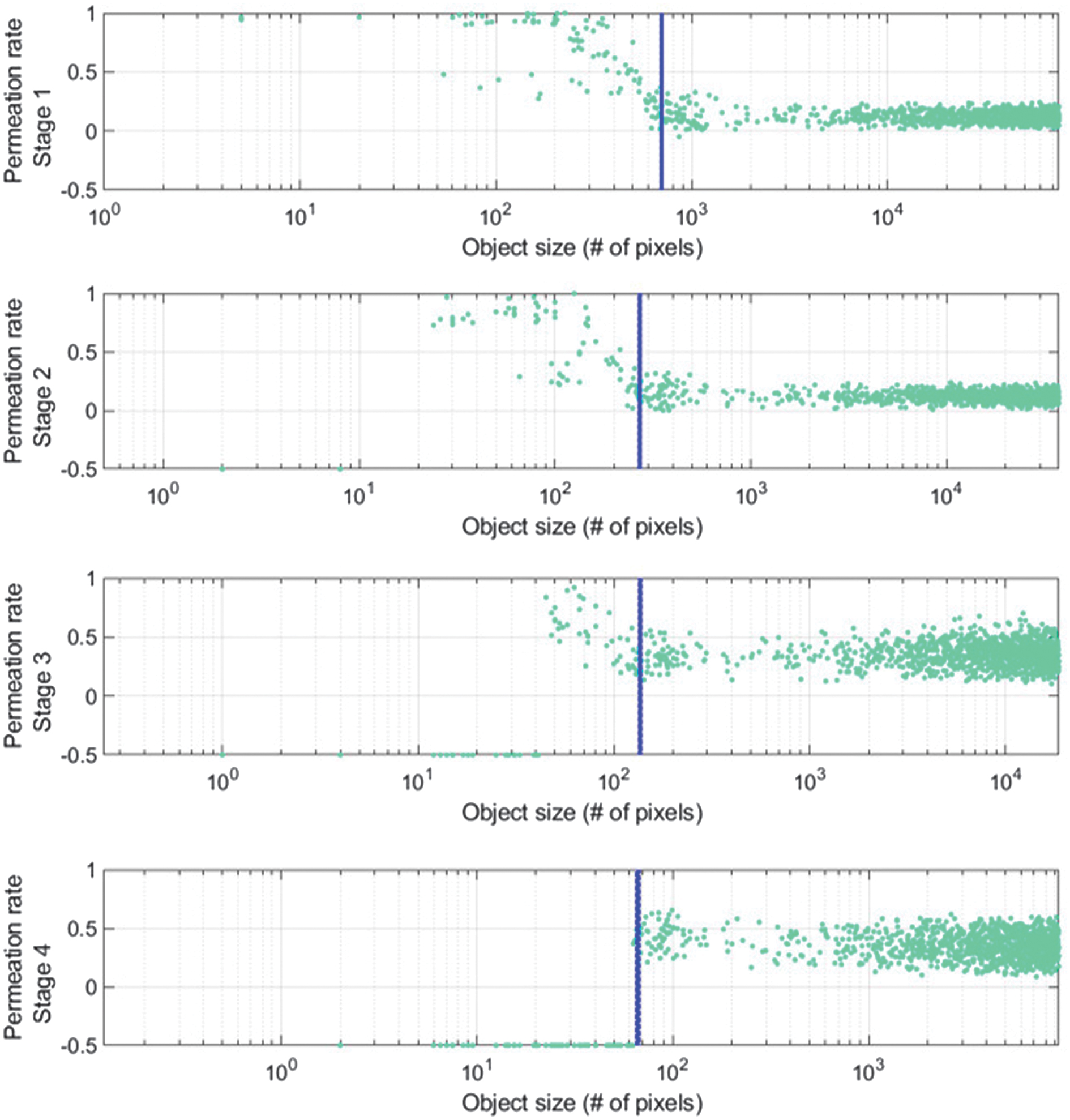 Fig. 3. The mU-Net”s permeation rate in relation to phases.
Upsampling, carried out through a layer of deconvolution along the residue path, as well as residual operation at the connection between skips, as illustrated in Fig. 2(d), automatically removes information based on object size. that is a signal in the remaining course after the suggested object-dependent upsampling, and that is a signal defined following the shortening by the omission of a convolution layer’s skip connection as follows by equations (10) and (11),
Where reversible convolution as , kernel weighting as w, bias worth as b and sampling set as θ in the skip link layer of residual path. All the weight, bias, kernel and sampling set in equation (11) are the complete set of convolutional layer parameters, where they are different from each other. Subsequently, the prior signal is characterized by equation (12) that is prior to the convolution process at the decoding stage and it is characterized in Fig. 2(d),From equation (12), adaptive filtering is used to filter feature data in the residual path in contrast to the traditional U-Net in equation (6). Let’s assume, for the sake of simplification, that adaptive up-sampling causes characteristics of the enormous object to be interpolated and features from the small object to be annihilated filtered at the early stage. The following are the results of the suggested network. By equations (13) and (14),
where cul+1 = 0.
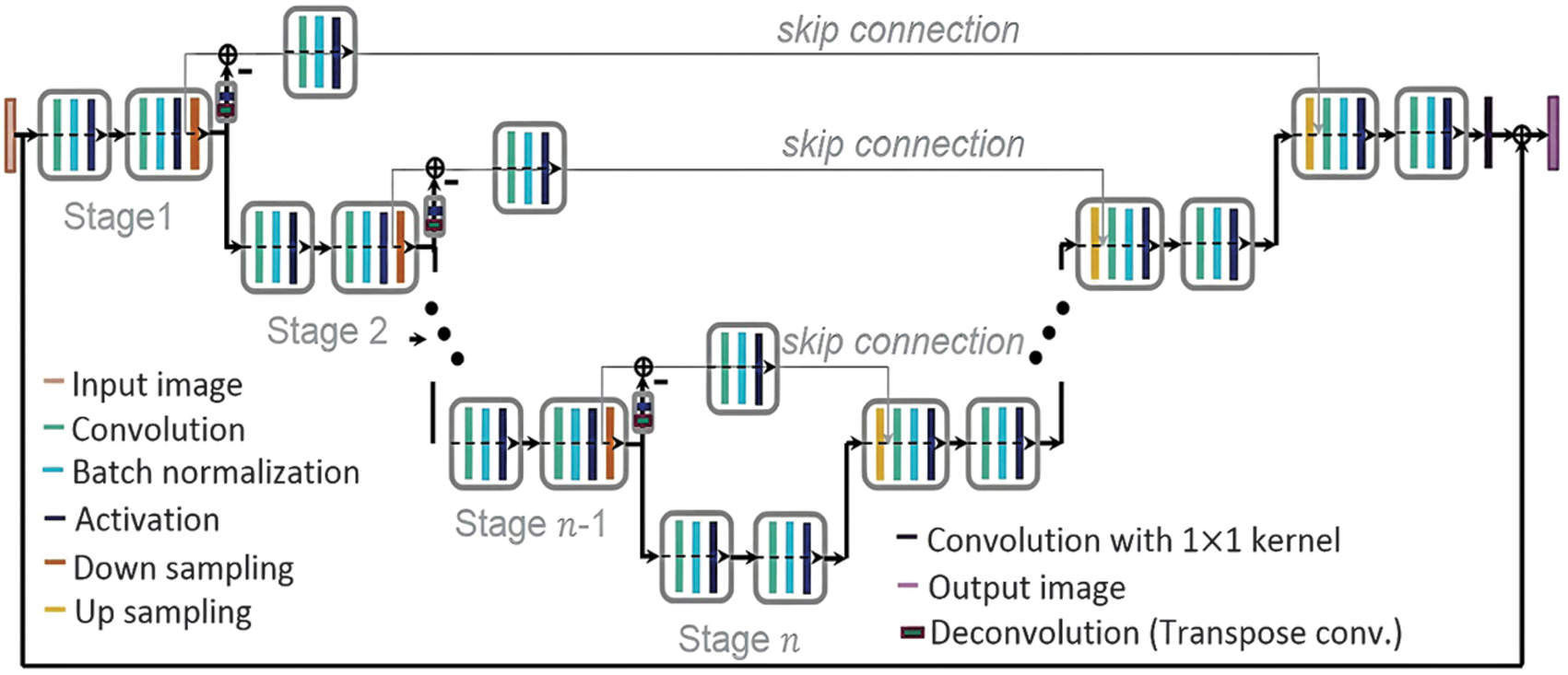
As seen in Fig. 3, edge-like information can be found in feature maps of large objects formed here after the residual pass in the bypassing connection. The suggested network extracts edge data for large objects with a preference that is matched to in equation (13). Contrarily, small object feature maps extract global features that are matched to the target better and do not have identical resolving losses as a normal U-net architecture (loss from deconvolution and pooling are absent) in equation (14). In addition, both and in equations (13) and (14) pass the further convolutional layer of for the purpose of extracting higher-level features, skipping the connection. The suggested network additionally makes use of weight decay, dropout, and batch normalization to increase accuracy. The suggested network’s loss function is defined as the mean square error (MSE) over the outputs of estimate and desired multi-class segmentation. Figure 4 shows the architecture of mU-Net segmentation [24].
D.SAM-ENet CLASSIFICATION
1.ENet MODEL
A new convolutional neural network called ENet was proposed by Google in May 2019. ResNet deepens the network primarily to improve accuracy. ENet balances the resolution, depth, and width of the network using compound scaling factors to improve accuracy and performance.
2.SAM ATTENTION MODULE
Various factors influence and complicate the topologies of various convolutional neural networks. SimAM, in comparison, considers the channel as well as the space. Without changing the original network’s parameters, three-dimensional attention weights are suggested. It develops a quickly convergent solution while defining a neuroscience-based energy function particularly. SimAM frequently outperforms the most common attention modules for SE and CBAM. SimAM can perform better than these two common categories of attention modules, as illustrated in Fig. 5 [25].
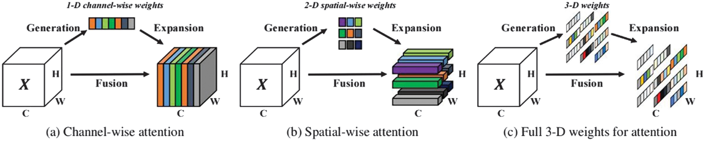 Fig. 5. Three different attention steps are compared.
The SimAM module establishes an energy function and searches for significant neurons. It adds regular words and binary labels. Finally, the following formula can be used to get the lowest energy by equation (15):
One of them, is the average neuronal value. is a measure of all neurons’ variance t, the intended neuron. the input feature’s channel has additional neurons. λ is a measure of regularization. You can determine how many neurons are present on that channel by M = H × W. In conclusion, energy plays a role in the distinction between neurons and neurons in the peripheral cortex. Each neuron”s importance can be determined by 1/e*. To fine-tune features, it employs a scaling operator. The SimAM module”s entire development process is shown in equation (17):
where E aggregates all e in the spatial and channel dimensions. To restrict the size of the value in E, sigmoid is used.3.SAM-ENet
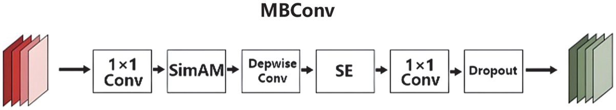
There is a 3 × 3 convolution layer in the first stage. MBConv, the most significant structural component of this network model, is present in the second through eighth stages. One-to-one convolution, pooling, and the final completely connected layers make up the final stage. MBConv is divided into five sections. A 1 × 1 convolution layer makes up the first component. A depth-wise convolution comes next and then the SE attention module. A 1 × 1 convolution layer is the fourth component, which reduces the number of dimensions. A dropout layer comes last as a solution to the overfitting issue, in order to boost the channel and spatial weights. Following the initial convolutional layer was the SimAM module. Figure 6 [26] depicts the fundamental structure of this paper, MBConv. It suitably modifies the remainder of the structure. The SE attention module is part of the original ENet. To make it better, our model incorporates the SimAM attention module.
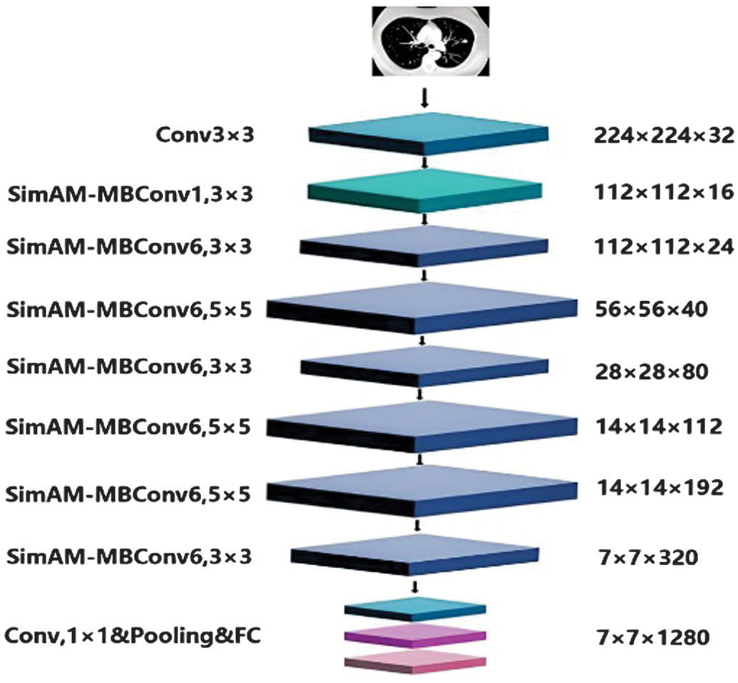
In this study, SAM-ENet is made up of two layers of convolution, one pooling layer and a single fully connected layer in addition to seven upgraded SAM-MBConv modules. In Fig. 7, different levels are represented by various colors and sizes. First, the pictures with the dimensions of 224 × 224 × 3 are ascended by the 3 × 3 convolutional layer. The size of the feature-filled images that were acquired is 112 × 112 × 32. The features of the photos are then extracted using SimAM-Conv. When two SimAM-Convs are identical, the connection is terminated and the input is established. After 1 × 1 The original channel is recovered using point-by-point convolution, and classification is performed on the fully linked layer.
4.WILDEBEEST HERD OPTIMIZATION ALGORITHM
The WHOA [27] has been used in this study to optimize our deep network, and it was chosen primarily because it is one of the more modern types of metaheuristic algorithms. The WHO algorithm was influenced by wildebeests’ foraging behavior, and its benchmark function findings, which were based on the research, likewise display superior results. This obliges us to utilize this metaheuristic approach to increase the effectiveness of the suggested CNN. Male sex challenges with rivals are used by wildebeests, a sociable mammal species that travels in search of food sources, in order to entice females for mating.
The WHO algorithm initializes a number of populations (wildebeests) at random as potential possibilities. There are only a few people in the lower classes (), and the higher () boundaries, i.e.,
where i = 1, 2, …, N.The wildebeest then employs the milling process to move about locally. The phase is depicted by continuing to search for the ideal position while taking into account a fixed number (n) is used as the little random movement that varies with the solution spaces, a haphazard phase Zn has been used by the applicants for position X to often look for the little random phase opportunities. The candidate results were adjusted using a random step size in a customizable length. The local experimentation phase as a result obtained as shown in the following equation (19):
where ɛ represents the factor affecting learning speed, the candidate number is described i, θ signifies a randomly generated, uniformly distributed number between 0 and 1, where defines a vector of random units.The wildebeest then adjusts its position to obtain the best possible random location after evaluating a fixed number (n) of unimportant candidates at random, i.e.,
where and elucidate the factors that the leaders will use to direct the candidates’ local movements.The previous step is to mimic the swarm instinct of wildebeests. Once the other contenders are situated in an area with an appropriate food source, this is mimicked, i.e.,
where establishes a random candidate, and indicate the factors that the leader will use to direct the crew’s local movement.There is additional term in the WHOA to prevent the candidates from traveling to areas with limited food sources. The mathematical model for this word is equation (22):
where describes a unit vector of randomness.The algorithm also includes a phrase for simulating busy areas. When the grass is fertile on a large scale, there is a throng. The name of this concept is “individual pressure.” This word allows a challenge to be completed and the strongest contender can destroy the others utilizing equation (23):
where η indicates a threshold so that people won’t swarm into the places and describes the approximate amount of exploitable components.The swarm social memory, which is simulated in the last stage to provide better placements, is obtained via the following methods equation (24):
The total output provides an overview of the system “Wildebeest Herd Optimization”.
- (1)setting up answers for the Wildebeest Herd. When hunting for the solution space, the source of the fertile grass, the herd follows the leader.
- (2)attempting to capture the most productive source of food for the wildebeest based on the algorithm’s conditions for exploitation and exploration.
- (3)As long as the termination conditions have not been met, all stages are repeated.
IV.RESULTS AND DISCUSSION
A.EXPERIMENTAL SETUP
On a desktop with an Intel Core i7-5960X, 32 GB of RAM, and two GTX 1080 graphics cards, experiments were run using Python 3.5 and Keras 2.2.
B.PERFORMANCE METRICS
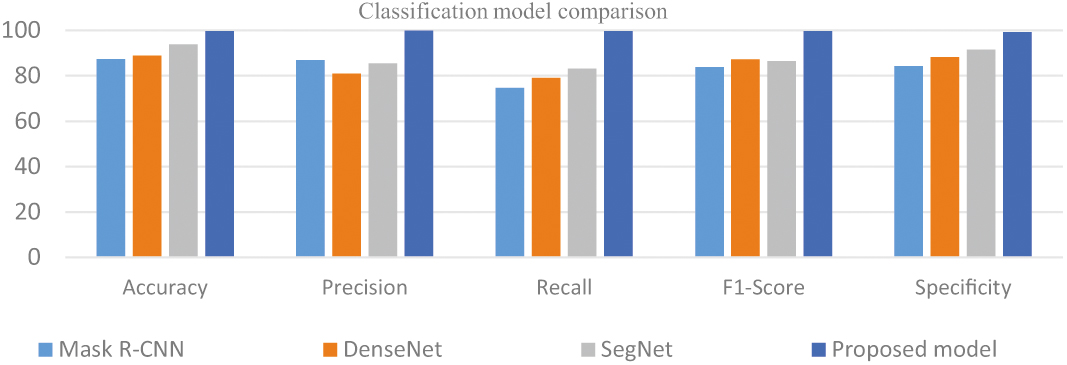
From Table I, Fig. 8, the mU-net model’s multi-scale, multi-modal approach assists in lowering false positives, a crucial component in lung nodule segmentation to assure correct diagnosis and lower the need for pointless treatments, which produces better results for the proposed model than for other models.
Table I. Comparison of segmentation models
| Models | Accuracy | Precision | Recall | F1-Score | Specificity |
|---|---|---|---|---|---|
| Mask R-CNN | 87.33 | 86.95 | 74.58 | 83.712 | 84.23 |
| DenseNet | 88.9 | 81.06 | 79.21 | 87.15 | 88.32 |
| SegNet | 93.79 | 85.47 | 83.22 | 86.43 | 91.54 |
| U-net | 95.16 | 89.11 | 89.45 | 90.65 | 95.86 |
| Proposed model | 99.76 | 99.85 | 99.68 | 99.66 | 99.32 |
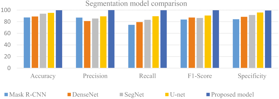 Fig. 8. Analysis of segmentation models.
Insights from Table II and Fig. 9, the proposed model achieved 98.2% of accuracy, 97% of precision, 97% of recall, 97.8% of F1-score and 97.5% of specificity, that shows better performance than the cited articles of ACO, GWO, and ABC Algorithms.
Table II. Models for classification are compared
| Models | Accuracy | Precision | Recall | F1-Score | Specificity |
|---|---|---|---|---|---|
| AlexNet | 86.5 | 87 | 86 | 86 | 86 |
| GoogleNet | 87.5 | 91 | 87 | 89 | 88 |
| ResNet-50 | 91.7 | 92.5 | 92.5 | 93.4 | 95 |
| VGG-16 | 94 | 94.2 | 95 | 94.6 | 96.3 |
| 98.2 | 97 | 97 | 97.8 | 97.5 |
V.CONCLUSION
Our research on lung nodule segmentation using the LIDC-IDRI dataset has yielded promising results and significantly improved the field of medical image analysis. This paper introduced the Bayesian threshold-based Taylor series technique for picture preprocessing. This paper developed a state-of-the-art technique to enhance lung nodule images while reducing noise. The segmentation method employed in this work, the mU-net design, is famous for being effective at segmenting medical images. These segmented lung nodules were categorized with the assistance of the cutting-edge neural network architecture SAM-ENet. This has a very high degree of classification accuracy for nodules. Our models were carefully calibrated and optimized for the task at hand using the innovative WHOA for hyperparameter tuning in this work. As a result of the experimental study, it was determined that the suggested model had segmentation and classification accuracy values of 99.76% and 98.2%, respectively. Even if the results of our recommended strategy were good, there is still room for advancement. Evaluations should be performed on large and diverse datasets to improve the system’s resilience.