JAIT

I.INTRODUCTION

Depending on their usage, ad hoc networks are mainly of four (4) types: wireless sensor networks (WSNs), wireless mesh networks (WMNs), vehicular ad hoc networks (VANETs), and mobile ad hoc networks (MANETs) [1]. In a MANET, communication happens through single and multiple hops based on the proximity of the nodes. Multiple hops enable communication between nodes that cannot connect directly [2]. Route selection at the network layer is a significant objective of any routing algorithm.

High-node mobility in MANETs eventually results in dynamic network structures; hence, managing routing resources is necessary [3]. One such resource is energy since the entities involved have limited battery life [4]. It is not always the case that the shortest route is the best one [5]. The best path is the shortest routing path using the least energy.

The intelligent network approaches used in MANETs, mainly for power-aware routing, are classified into four (4): machine learning-based, fuzzy logic-based, metaheuristic-based, and game theory-based approaches.

Machine learning-based approaches use techniques in machine learning such as supervised learning (e.g., neural networks), unsupervised learning (e.g., clustering), reinforcement learning, and deep learning. Routing algorithms of this approach include LASEERA, a stable and energy-efficient routing algorithm based on learning automata theory for MANET [6], and concatenation of convolutional layer with a max-avg pooling layer in a deep convolutional neural network (CCMAP-DCNN) [7]. Substantial datasets are required for training, which may not be readily available when implementing machine learning approaches in routing algorithms in dynamic and resource-constrained environments such as MANETs.

Fuzzy logic-based approaches provide dynamic adaptations during uncertainties when used for developing energy-efficient routing algorithms. Routing algorithms in this class include the fuzzy energy-based routing protocol-AODV (FERS-AODV) [8] and the fuzzy approach-based stable energy-efficient AODV (Fuzzy AODV) [9]. Even though fuzzy logic is highly successful in dealing with uncertainty and imprecision, sometimes it cannot manage challenging situations with complex rules. For instance, the rules may explode in MANET scenarios with numerous nodes and varying conditions.

Game theory-based approaches give a structured method to model interactions among nodes in MANETs as a game, focusing on aspects such as coalition formation, incentive mechanisms, etc. Routing algorithms in this category include the game theory-based energy-efficient routing (GTEER) [10] and the modified OLSR [11]. Even though game theory approaches foster equity by discouraging selfish nodes from draining extreme energy, they are required to compute very complex payoff functions and equilibria, which may decrease their performance. Furthermore, the accuracy of the MANETs state data impacts their effectiveness.

Metaheuristics find near-optimal solutions to an optimization problem [12]. Typical power-aware routing algorithms of this type are the power-aware river formation dynamics routing algorithm (PRFDRA) [13] and the power-aware intelligent water drops routing algorithm (PIWDRA) [14], which are based on finding energy-efficient routing paths using intelligent water drops (IWD) and river formation dynamics (RFD), respectively. These algorithms are mostly nature-inspired [15]. Most of these routing algorithms’ nature-inspired mimicking and stochastic abilities make them highly effective at finding feasible solutions quickly.

The IWD, proposed by Dr Shah-Hosseini, is a metaheuristic inspired by the behavior of water drops in nature. In this approach, each water drop represents a potential solution to the optimization problem. The movement of water drops is guided by a combination of problem-specific information and random exploration. Initially, the water drops are randomly distributed across the problem space. As the algorithm progresses, water drops adjust their positions based on local information and the quality of nearby solutions. This process is iterated until a satisfactory solution is found or a termination criterion is reached [16–19].

The RFD, proposed by Rabanal et al. in 2007, is a metaheuristic inspired by the natural process of river formation. In this approach, potential solutions to an optimization problem are represented as rivers in a landscape. The optimization process mimics the erosion and sedimentation processes in rivers, where rivers evolve to find optimal paths. In the beginning, the landscape is randomly created, and rivers flow through it, gradually carving out pathways of least resistance. As the algorithm progresses, the paths are refined based on the quality of the solutions they lead to. This iterative process continues until convergence or a termination criterion is obtained [20–22].

Hybrid metaheuristics have recently gained popularity since it is widely recognized that combining various algorithms can improve performance by taking advantage of the strengths of each algorithm [23]. This research aims to hybridize the IWD and RFD metaheuristics for optimizing routing path selection with minimum energy. The rest of the paper is organized as follows: Section II reviews related work on hybrid metaheuristic routing paths in MANETs. Section III presents the proposed approach. Section IV gives the performance evaluation, and Section V concludes the paper.

II.RELATED WORKS

Goswami et al. [24] proposed a hybrid metaheuristic approach for energy-efficient routing in MANETs, emphasizing security and energy efficiency. The approach combines the hybrid sailfish optimizer and whale optimization algorithm (HS-WOA) to optimize parameters such as energy consumption, remaining battery energy, link cost, energy cost per packet, path loss, packet delivery ratio, end-to-end delay, and routing overhead ratio. However, including many constraints may increase the computational burden and overhead.

Prabha and Senthil [25] proposed enhancements to the ad hoc on-demand multipath distance vector (AOMDV) routing protocol for MANETs, integrating link availability estimates for seamless route handoff without considering energy aspects. They combined the bat algorithm (BAT) with harmony search (HS) to address BAT’s tendency for narrow solutions by leveraging HS’s exploration capabilities to diversify the solution space and prevent local optima.

Priya and Suganthi [26] introduced the AOMDV protocol, which integrates the grey wolf optimizer (GWO) with differential evolution (DE) and firefly (FF) algorithms to resolve routing conflicts in MANETs, although energy considerations are overlooked. AOMDV utilizes routing data from AODV to minimize overhead associated with path discovery. The protocol balances exploration and exploitation, enhancing convergence speed and solution accuracy.

Hadi and Makki [27] introduced hybrid cat and particle swarm optimization (CPSO), a system combining cat swarm optimization (CSO) with particle swarm optimization (PSO) algorithms to enhance MANET routing optimization without considering energy aspects. CPSO utilizes CSO for the initial search, switches to PSO upon CSO stagnation, and reverts to CSO using the current best solution if PSO also stagnates. Parameters remain unchanged during switches, and the system restarts if both algorithms fail to improve the solution.

Alappatt et al. [28] proposed a trust-based, energy-efficient multipath routing mechanism for MANETs, employing the levy flight-centered shuffled shepherd optimization (LF-SSO) algorithm to optimize paths based on trust values, residual energy, and path distance. However, for the energy aspect, focusing solely on the maximum residual energy of nodes may lead to uneven energy depletion and ineffective load balancing.

Srilakshmi et al. [29] introduced the genetic algorithm with hill climbing (GAHC) routing protocol for MANETs, integrating a fuzzy C-means algorithm to identify cluster leaders and optimize paths. For the energy aspect, reliance solely on a node’s remaining energy may lead to premature depletion in critical nodes.

Kaliyamurthi and Palanisamy [30] introduced the hybrid firefly and galactic swarm optimization (HFFGSO). This routing approach combines FF and galactic swarm optimization (GSO) methods to address routing void challenges in the geographical routing protocol (GRP). While effectively optimizing routes, the reliance on channel mechanisms for energy aspects may increase computational complexity and communication overhead.

Chandrasekaran and Selvaraj [31] introduced a QoS routing strategy for MANETs, combining DE and FF algorithms into the AODV protocol to optimize QoS performance. While the algorithm considers factors such as hop count, remaining energy, and routing load, relying solely on node energy for the energy aspect may lead to premature depletion, especially at critical nodes.

Hussein and Dahnil [32] proposed the eligible energetic path (ALEEP) for MANETs, integrating ant colony optimization (ACO) and the lion optimization algorithm (LOA). ACO identifies potential paths relying mainly on transmission power, which may overlook energy consumption variations from other factors. Moreover, LOA selects the top two based on energy levels, potentially leading to the over-depletion of critical nodes.

Kumaran and Ramasamy [33] proposed the energy-efficient ACO GA hybrid metaheuristic (EAGHM) for enhancing energy efficiency in MANETs. By integrating ACO and genetic algorithm (GA), the hybrid approach considers QoS metrics such as residual node energy, end-to-end delay, bandwidth, and hop count. ACO establishes routes based on delayed pheromone concentrations and hop counts, forming the initial population for GA, which further optimizes routes using a fitness function incorporating genetic operations. Relying solely on node energy for the energy aspect may lead to premature depletion in critical nodes.

Amin [34] introduced SMART, a MANET routing system merging ACO and RFD techniques. SMART employs ACO for route establishment based on RFD principles, utilizing data packets for congestion management and incorporating learning mechanisms for adaptation to network environments. Despite its comprehensive approach, SMART overlooks energy considerations and does not base move drop probability on climbing drops in RFD.

Sujitha and Nivetha [35] proposed a routing optimization approach that combines ACO and GA techniques. GA guides the routing path selection, while ACO facilitates route discovery using pheromone values related to nodes, linkages, delay, and data transfer suitability. These values contribute to computing multiple paths, with GA identifying the optimal route based on QoS parameters such as hop count, bandwidth, and delay. Notably, the algorithm does not consider energy aspects.

Jamali and Sajjad [36] proposed BA-TORA to mitigate load imbalance issues in MANETs caused by TORA’s preference for minimum-hop routes. BA-TORA integrates bee and ant algorithms to distribute traffic evenly and select energy-efficient routes. For energy, sending data over paths with high energy levels may result in uneven energy depletion among nodes.

III.METHODOLOGY

A.FORMULATION OF PROBLEM

The problem domain of MANETs is conceptualized as a connected, undirected graph $G = (V_{N}, E$ ). In the graph, each vertex denotes a node. The set of all nodes in the network is denoted by $V_{N}$ . In the network representation, an edge symbolizes a connection between two nodes. The set of all edges is given as $V_{N} (V_{N} - 1) / 2$ . The set of all links in the network is denoted E. The transmission range and distance between adjacent nodes are denoted as “r” and “d,” respectively. A two-way link $e (e ε E)$ exists between two adjacent nodes if $d \leq r$ . The collection of all possible paths originating from the source node s $(s ε V)$ leading to the targeted node $t$ $(t ε V)$ is represented as $P$ . The set of all edges and nodes of any given path $p (p ε P)$ is represented as $E (p)$ and $V (p)$ , respectively. Table I gives the nomenclatures.

Table I. Nomenclature and their meaning

Nomenclature
Static parameters	Meaning
$G (V, E)$	A graph G is made up of $V_{N}$ number of nodes and connected with $E$ number of edges
$q {(T)}^{T B} = - \infty$	Quality of total best solution
${iter}_{\max} = 100$	Maximum number of iterations
${iter}_{count} = 0$	Current iteration number
$a_{v} = 10.00$ , $b_{v} = 0.01$ , $c_{v} = 1$	Velocity updating parameters
$a_{s} = 10.00$ , $b_{s} = 0.01$ , $c_{s} = 1$	Soil updating parameters
$p r o b (i, j; D r o p)$	Probability of drop choosing to move from node $i$ to $j$
$Init S o i l = 10000$	Initial soil assigned at the edges
$Init V e l = 200$	The initial velocity of the originating drop
$N_{Drop} = 250$	Number of drops
$ɛ_{s}$ = 1.0	A small positive constant
$ρ^{Drop} = 0.9$	Global soil updating parameter
$ρ_{n} = 0.9$	Local soil updating parameter
Dynamic parameters	Meaning
$V_{c} D r o p = {}$	Visited nodes of drop
$i n i t V e l = v e l^{Drop} (t)$	Velocity of each drop
$soi l^{Drop} = 0$	Initial soil of drops
Other parameters	Meaning
$H U D$	Heuristic undesirability function
$Δ s o i l (i, j)$	Change of soil between the edge of nodes $i$ and $j$
$c o s t (i, j)$	Cost function/path cost
$f (s i l (i, j))$	Goodness of soil
$g (s o i l (i, j))$	Function for shifting $s o l (i, j)$ values
$Δ VelDrop$	Change velocity of a drop
$V_{N}$	Number of nodes in the MANET
$T^{Drop}$	Solution at the end of each iteration
$T^{I B}$	Total best solution throughout your iterations
T^TB	Total best solution of current solutions
$σ = 0.02$ , $μ = 0.06$ , and $τ = 0.02$	Constant parameters in $cost (i, j)$
$a l t i t u d e (S) = 1000$ , $a l t i t u d e (I) = 10000$ , $a l t i t u d e (D) = 0$	Altitude of source, intermediate and destination nodes
$T D$ , E, and $N_{Hops}$	Time delay, energy, and number of hops
$V_{k} (i)$ , $U_{k} (i)$ , and $F_{k} (i)$	Set of neighbors with a positive, negative, and flat gradient
sum	The sum of the weights of the various collections
$ω = 0.01$ , $δ = 0.01$	Specific fixed small values in $sum$
$ɛ_{V}$ , $ɛ_{U}$ , $ɛ_{F}$	Parameters associated with positive, negative, and flat gradients, respectively, in $e r o s i o n (i, j)$
$β = 0.1$	A constant to control the amount of sediment deposit
$P_{k} (i, j)$	Probability of k assessing node j from i
max(prob)	Maximum probability
$g r a d i e n t (i, j)$	The gradient along the path from node $i$ to $j$
$a l t i t u d e (i)$	Altitude of the eroded node $i$
$e r o s i o n (i, j)$	Erode node along the path from $i$ to $j$
$s e d i m e n t (i, j)$	Sediment of the Drop added to the altitude of node $j$
$param B l o c k e d D r o p = 1$	Parameter for a blocked Drop
$c a r r i e d S e d i m e n t (i, j)$	Sediment carried by the Drop from node $i$ to $j$

B.HYBRID POWER-AWARE INTELLIGENT RIVER-ROUTING ALGORITHM (HPIRRA)

This algorithm combines elements of IWD and RFD, using hybrid control agents called drops that possess characteristics from both approaches. IWD plays a crucial role in multiple route selection by incorporating factors such as energy, hop count, and time delay into its mechanisms. Similarly, RFD complements IWD to select the best path in each iteration, incorporating the same factors as IWD. In the algorithm, a fitness or objective function evaluates the quality of each solution, aiming to find the optimal solution in each iteration. The objective function is represented as the minimization cost function denoted as $cost (i, j)$ and it integrates metrics including time delay (TD), minimum energy ( $Min (E)$ ), and the number of hops (N_Hops), all derived from the path’s nodes. Concerning $Min (E)$ , the routing algorithm should select a path that has the maximum value of the minimum energy that a node has in a path across all possible paths. By calculating the path cost for each drop, the fitness function ranks the solutions and identifies the one with the minimum cost as the best. The path is then checked for optimality based on the cost function provided in equation (1). With IWD aid, the best total solution is selected based on the quality of the solutions generated at the end of all the iterations. Furthermore, HPIRRA assesses nodes based on their battery life remaining. The algorithm shuns critically low energy levels. It switches to a different path if a node’s energy drops to a 30% threshold. Figure 1 provides the flowchart of the algorithm.

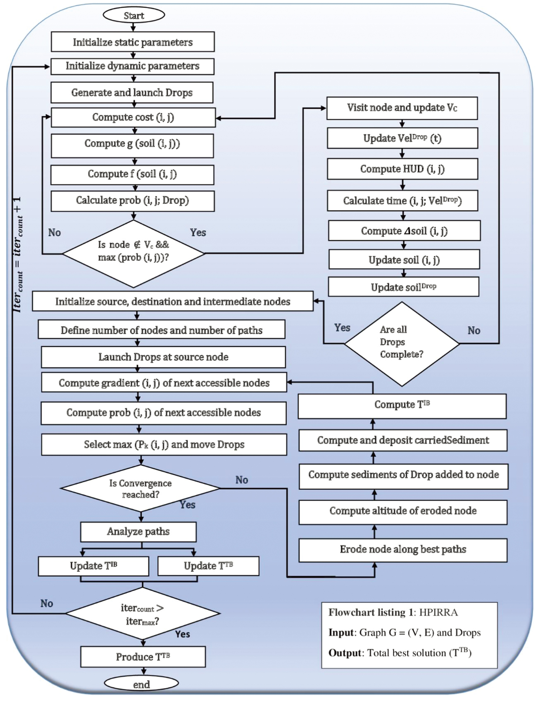Fig. 1. Flowchart of HPIRRA Performance Evaluation.

Input: $G r a p h G = (V_{N}, E)$ and Drops

Output: Total best solution (T^TB)

1: Initialize the static parameters

2. Initialize the dynamic parameters

3: Generate Pop

4: while ( ${iter}_{count} \leq i t e r_{\max}$ ) do

5: for (each Drop)

6: Update $V_{c}$

7: for (each Node $\notin$ $V_{c}$ )

8: Compute $cost (i, j)$ using eq (1)

9 : cost (i, j) = σ \times TD + μ \times \frac{1}{Min (E)} + τ \times \frac{1}{N_{Hops}}

(1)

10: Compute $g (soil (i, j))$ using eq (2)

11 : g (s o i l (i, j)) = {\begin{matrix} s o i l (i, j) i f \min (s o i l (i, j)) \geq 0 \\ s o i l (i, j) - \min (s o i l (i, l)) e l s e \end{matrix}

(2)

12: Compute $f (soil (i, j))$ using eq (3)

13 : f (s o i l (i, j)) = \frac{1}{ɛ_{s} + g (soil (i, j)) + c o s t (i, j)}

(3)

14: Calculate $prob (i, j; Drop)$ using eq (4)

15 : p r o b (i, j; D r o p) = \frac{f (soil (i, j))}{Σ_{k \neq V_{c (Drop)} f} (soil (i, k))}

(4)

16: Select the node with max(prob)

17: end for

18: for (each Node $\in$ $V_{c}$ )

19: Update ${vel}^{Drop} (t)$ using eq (5)

20 : v e l^{Drop} (t + 1) = v e l^{Drop} (t) + \frac{a_{v}}{b_{v} + c_{v .} s o i l^{2} (i, j)}

(5)

21: Compute $H U D (i, j)$ using eq (6)

22 : H U D (i, j) = \frac{T D (i, j)}{E (j)}

(6)

23: Calculate $time (i, j; {vel}^{Drop})$ using eq (7)

24 : t i m e (i, j; v e l^{Drop} (t + 1)) = \frac{H U D (i, j)}{v e l^{Drop} (t + 1)}

(7)

25: Calculate $Δ soil (i, j)$ using eq (8)

26 : Δ s o i l (i, j) = \frac{a_{s}}{b_{s} + c_{s} . t i m e^{2} (i, j; v e l^{Drop} (t + 1))}

(8)

27: Update $soil (i, j)$ using eq (9)

28 : s o i l (i, j) = (1 - ρ_{n}) . s o i l (i, j) - ρ_{n} . \frac{Δ s o i l (i, j)}{N_{Hops} . E}

(9)

29: Update soil^Dropusing eq (10)

30 : {soil}^{Drop} = {soil}^{Drop} + \frac{Δ s o i l (i, j)}{N_{Hops} . E}

(10)

31: end for

32: end for

33: UpdateT^IBby repeating steps 34 to 61

34: Initialize S, D and I nodes

35: Define the number of nodes, number of paths

36: Generate Pop

37: while ( $i t e r_{count} \leq i t e r_{\max})$ do

38: for (each Node)

39: Compute $g r a d i e n t (i, j)$ using eq (11)

39 : g r a d i e n t (i, j) = \frac{(altitude (i) - a l t i t u d e (j)) . T D_{j}}{E_{j} . N_{Hops} (i, j)}

(11)

40: Compute sum using eq (12)

41:

s u m = (\sum_{l \in V_{k (i)}} g r a d i e n t (i, l) . T D_{j}) + \sum_{l \in U_{k}} (\frac{ω . T D_{j}}{| gradient (i, l) |}) + \sum_{l \in F_{k (i)}} (δ . T D_{j})

(12)

42: Compute $P_{k} (i, j)$ using eq (13)

43 : P_{k} (i, j) = {\begin{matrix} \frac{gradient (i, j) . T D_{j}}{sum . E_{j} . N_{Hops (i, j)}}, & f o r j \in V_{k} (i) \\ \frac{(ω / | gradient (i, j) |) . T D_{j}}{sum . E_{j} . N_{Hops (i, j)}}, & f o r j \in U_{k} (i) \\ \frac{δ . T D_{j}}{sum . E_{j} . N_{Hops (i, j)}}, & f o r j \in F_{k} (i) \end{matrix}

(13)

44: Select Node with maximum ( $P_{k} (i, j)$ ) and move

45: if (Convergence is not reached)

46: Analyze paths

47: Perform erosion (i, j) using eq (14)

48:

e r o s i o n (i, j) = {\begin{matrix} \frac{ɛ_{V} . g r a d i e n t (i, j) . T D_{j}}{(V_{N} - 1) . N_{Drops} . E_{j} . N_{Hops} (i, j)}, & f o r j \in V_{k} (i) \\ \frac{ɛ_{U} . T D_{j}}{| gradient (i, j) | . (V_{N} - 1) . E_{j} . N_{Hops (i, j)}}, & f o r j \in U_{k} (i) \\ \frac{ɛ_{F} . T D_{j}}{(V_{N} - 1) . N_{Drops} . E_{j} . N_{Hops (i, j)}} & f o r j \in F_{k} (i) \end{matrix}

(14)

49: Compute altitude using eq (15)

50 : a l t i t u d e (i) = a l t i t u d e (i) - \frac{erosion (i, j)}{V_{N}}

(15)

51: Compute sediment (i, j) using eq (16)

52:

s e d i m e n t (i, j) = \frac{β . (altitude (i) - a l t i u d e (j)) . c a r r i e d S e d i m e n t (i, j) . T D_{j}}{E_{j} . N_{Hops} (i, j)}

(16)

53: Compute carriedSediment using eq (17)

54:

c a r r i e d S e d i m e n t (i, j) = c a r r i e d S e d i m e n t (i, j) + e r o s i o n (i, j) - s e d i m e n t (i, j)

(17)

55: Deposit CarriedSediment using eq (18)

56 : a l t i t u d e (j) = a l t i t u (j) + \frac{erosion (i, j)}{V_{N}}

(18)

57: if (Drop is blocked), use eq (19)

58:

a l t i t u d e (j) = a l t i t u d e (j) + p a r a m B l o c k e d D r o p . c a r r i e d s e d i m e n t

(19)

59: Compute $T^{I B}$ using eq (20)

60 : T^{I B} = a r g m i n \forall T^{Drop} c o s t (i, j)

(20)

61: end if

62: end if

63: UpdateT^TBusing eq (21)

64:

T^{T B} = = {\begin{matrix} T^{T B} & i f q (T^{T B}) \geq q (T^{I B}) \\ T^{I B} & o t h e r w i s e \end{matrix}

(21)

65: ${iter}_{count} + +$

66: end while

67: ProjectT^TB

IV.PERFORMANCE EVALUATION

A.SIMULATION SET-UP

HPIRRA is compared with the PRFDRA, the PIWDRA, the AODV routing protocol, and the destination sequence distance vector (DSDV) routing protocol under NS-3.37 simulations.

The strategies are implemented under two scenarios (refer to Table II). In the first scenario, the pause time intervals varied from 0 to 200 seconds in 40-second intervals. In the second scenario, the network’s node count is changed while maintaining a constant node density, ranging from 50 to 250 nodes. About one-third of the populace serves as sources; for instance, 15 for every 50, 30 for 100, 45 for 150, 50 for 200, and 75 for 250, producing an equal share across all scenarios. The base configuration (refer to Table III) remains the same.

Table II. Summary of all scenario settings

Simulation parameter	Scenario 1(Pause times)	Scenario 2(No of nodes)
No of nodes	250	50, 100, 150, 200, 250
Pause time (s)	0, 40, 80, 120,160, 200	40
Sources (nodes)	40	15 (50),30 (100),45 (150),60 (200),75 (250)

Table III. Summary of base settings

Simulation parameters	Value(s)
NS-3 Version	3.37
Mobility model	Random waypoint
Radio propagation model	Two-ray ground reflection model
Antenna model	Omni direction
Radio frequency	2.47 GHz
Application agent	FTP
Traffic	CBR
CBR traffic model	32Kbps
Transport agent	TCP
Network layer protocols	HPIRRA, PRFDRA, PIWDRA, AODV, DSDV
Initial node energy	100 Joules
Bandwidth	11 Mbps
Data packet generation rate	2 to 8 packets/second
Transmission power	3 Watts
Receiving power	1.5 Watts
Sleep power	0.6 Watts
Idle power	0.05 Watts
Default transmission range	250 Meters
Antenna power	1.5 Watts
Control packet size	8 Bytes
Data packet size	512 Bytes
Queue length/node maximum buffer size	25600 KB (i.e., 50 data packets)
Primary queue type	Drop tail queue
Simulation time	1500 Seconds
Terrain dimension	1500 meters square
Node speed	10 meters per second
Traffic pattern	Unicast

B.NETWORK PERFORMANCE METRICS

The metrics used are briefly explained:

▪Packet Delivery Ratio (PDR): PDR is the ratio of the number of data packets received at the destination to the number passed on [37].
▪Average End-to-End Delay (AE2ED): The average time spent by a packet to get to the destination from the sender [38].
▪Energy Consumption (EC): EC is the overall energy consumed by network entities during the experiment [39].
▪Network Lifetime (NL): NL is the time between the start and end of the network. For this research, it ends when the first node dies as a result of battery exhaustion [40].

V.RESULTS AND DISCUSSION

A.SCENARIO 1: IMPACT OF THE PAUSE TIME VARIATION

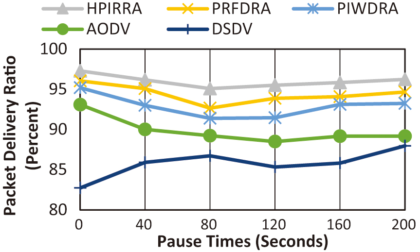
1).PACKET DELIVERY RATIO

Figure 2 displays the graph of the packet delivery ratio against varying pause times. The improvement rates of HPIRRA over PRFDRA, PIWDRA, AODV, and DSDV are 1.62%, 3.12%, 6.16%, and 10.28%, respectively. The average PDR for HPIRRA is increasing and has risen as high as 97.27%.

Fig. 2. PDR versus pause times.

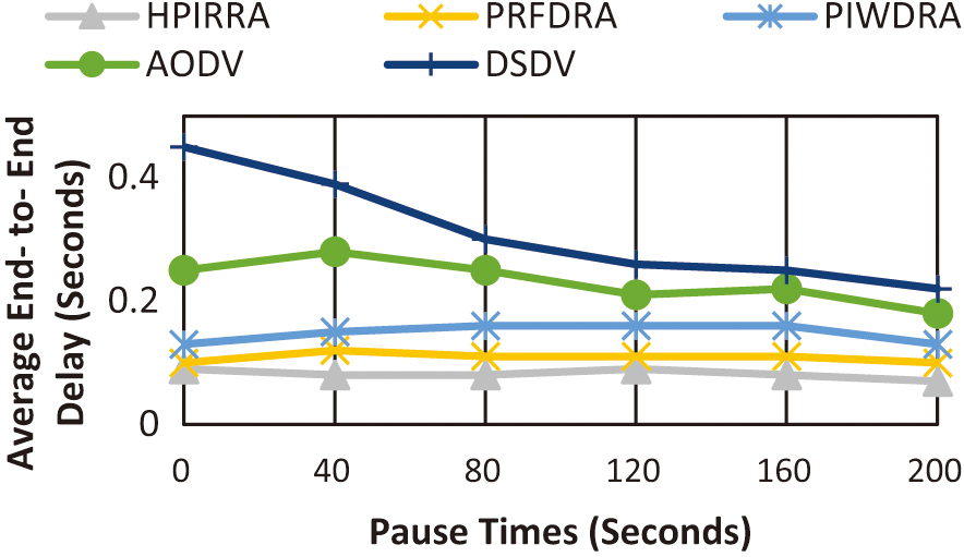
2).AVERAGE END-TO-END DELAY

A graph is created to show the relationship between AE2ED and different pause times, as displayed in Figure 3. The improvement rates of HPIRRA over PRFDRA, PIWDRA, AODV, and DSDV in seconds are 0.03, 0.07, 0.15, and 0.23, respectively. HPIRRA had the best average performance of 0.082 seconds, while DSDV lags. The highest delay performance of 0.07 seconds occurred with HPIRRA at a 200-second pause time.

Fig. 3. AE2ED versus pause times.

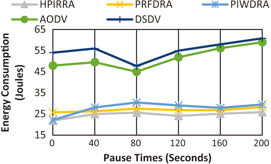
3).ENERGY CONSUMPTION

In Figure 4, a graph is constructed to show the relationship between energy consumption and varying pause times. The improvement rates in joules of HPIRRA over PRFDRA, PIWDRA, AODV, and DSDV are 2.32, 3.28, 26.96, and 30.66. HPIRRA had the highest average performance of 24.59 joules, while DSDV had the lowest average performance of 55.25 joules. The highest performance of 21.86 joules occurred with HPIRRA at 0 seconds.

Fig. 4. EC versus pause times.

4).NETWORK LIFETIME

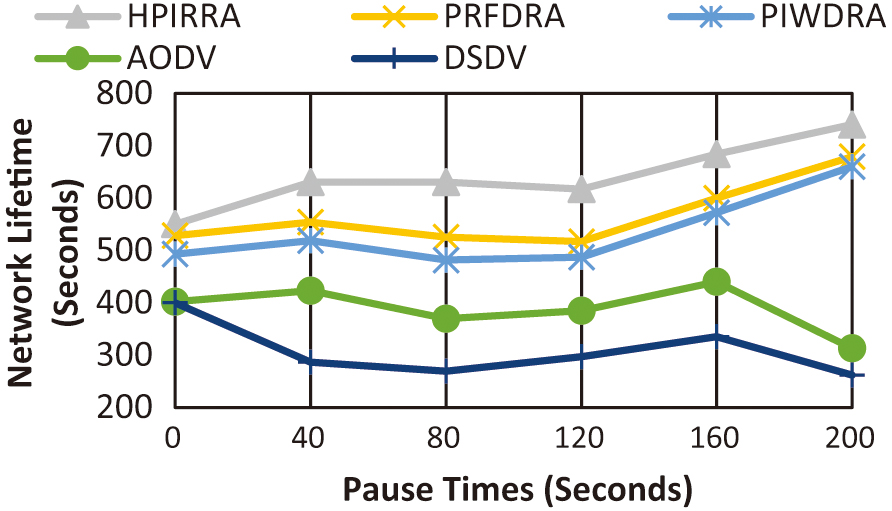
Figure 5 displays the relationship between network lifetime and varying pause times. The improvement rates in seconds of HPIRRA over PRFDRA, PIWDRA, AODV, and DSDV, respectively, are 74.86, 106.73, 253.25, and 333.95. HPIRRA exhibited the maximum NL of 740.71 seconds at 200 pause times.

Fig. 5. NL versus pause times.

B.SCENARIO 2: IMPACT OF VARYING THE NUMBER OF MOBILE NODES

1).PACKET DELIVERY RATIO

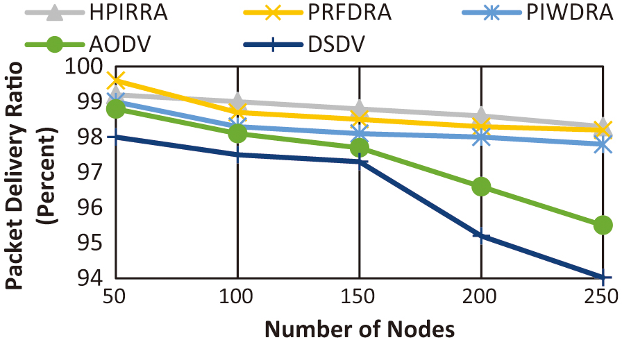
The correlation between PDR and different node counts is depicted in Figure 6. The improvement rates of HPIRRA over PRFDRA, PIWDRA, AODV, and DSDV, respectively, are 0.12%, 0.54%, 1.44%, and 2.38%. Among the five, HPIRRA emerged as the top performer, with an average performance of 98.78%. HPIRRA, PRFDRA, and PIWDRA mostly achieved performances above 98%.

Fig. 6. PDR versus number of nodes.

2).AVERAGE END-TO-END DELAY

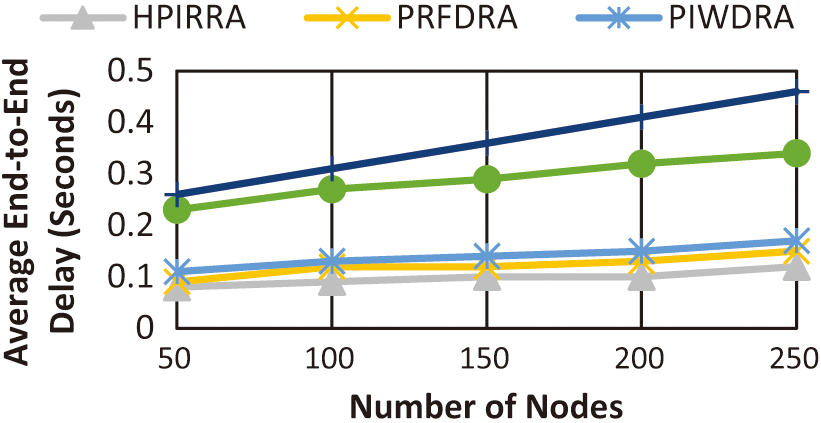
Figure 7 illustrates the association between AE2ED and various node counts. The improvement rates in seconds when comparing HPIRRA over PRFDRA, PIWDRA, AODV, and DSDV are, respectively, 0.02, 0.04, 0.19, and 0.26. HPIRRA outperformed all others with an average delay of 0.12 seconds. The optimum delay performance of 0.08 seconds occurred with HPIRRA with 50 nodes.

Fig. 7. AE2ED versus number of nodes.

3).ENERGY CONSUMPTION

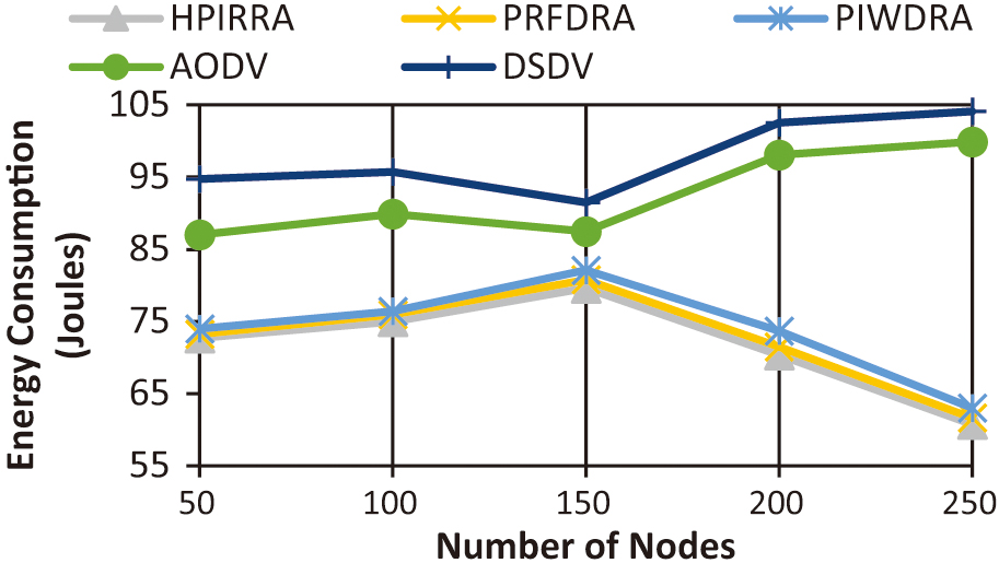
A graph illustrating the correlation between energy consumption and changing node counts is depicted in Figure 8. The improvement rates in joules of HPIRRA over PRFDRA, PIWDRA, AODV, and DSDV, respectively, are 0.94, 2.17, 20.8, and 23.42. HPIRRA had the maximum average EC performance of 71.67 joules. The least and maximum energy consumption occurs, respectively, with HPIRRA and DSDV at peak density.

Fig. 8. EC versus number of nodes.

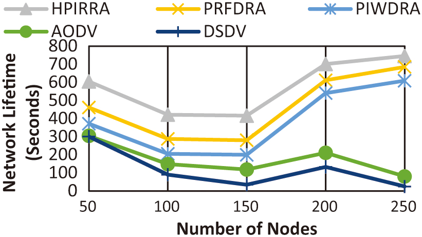
4).NETWORK LIFETIME

Figure 9 displays the relationship between network lifetime and the varying number of nodes. The improvement rates in seconds of HPIRRA over PRFDRA, PIWDRA, AODV, and DSDV, respectively, are 112.76, 192.53, 405.39, and 461.06. The highest NL of 745.71 seconds occurred with HPIRRA with 250 nodes.

Fig. 9. NL versus number of nodes.

VI.CONCLUSION

This study presented the HPIRRA strategy for efficient routing path selection with minimal energy consumption. By combining IWD and RFD algorithms, HPIRRA efficiently established multiple routes and selected optimal paths based on hop count, energy, and time delay. The selection of the global best path in HPIRRA relied on a cost function that prioritized minimum energy, hop count, and time delay, with minimum energy having the highest weight. Comparative analysis against existing algorithms, including PRFDRA, PIWDRA, AODV, and DSDV, illustrated that HPIRRA outperformed in packet delivery ratio, average end-to-end delay, energy consumption, and network lifetime. Future research directions may explore additional enhancements and the algorithm’s adaptability. Artificial intelligence techniques, such as machine learning and training, will also be the focus of future research.

Hybridizing Intelligent Water Drops and River Formation Dynamics for Optimal Routing Path Selection with Minimum Energy in MANETs

I.INTRODUCTION

II.RELATED WORKS

III.METHODOLOGY

A.FORMULATION OF PROBLEM

B.HYBRID POWER-AWARE INTELLIGENT RIVER-ROUTING ALGORITHM (HPIRRA)

IV.PERFORMANCE EVALUATION

A.SIMULATION SET-UP

B.NETWORK PERFORMANCE METRICS

V.RESULTS AND DISCUSSION

A.SCENARIO 1: IMPACT OF THE PAUSE TIME VARIATION

1).PACKET DELIVERY RATIO

2).AVERAGE END-TO-END DELAY

3).ENERGY CONSUMPTION

4).NETWORK LIFETIME

B.SCENARIO 2: IMPACT OF VARYING THE NUMBER OF MOBILE NODES

1).PACKET DELIVERY RATIO

2).AVERAGE END-TO-END DELAY

3).ENERGY CONSUMPTION

4).NETWORK LIFETIME

VI.CONCLUSION

CONFLICT OF INTEREST STATEMENT

REFERENCES