JAIT

I.INTRODUCTION

In the past 10 years, the Internet of Things industry has developed rapidly. With the reduction in size, performance, and cost of various sensors and electronic devices, these electronic components have become more widely used in life. Especially, the research on wearable smart devices, hair activity recognition, and human activity recognition (HAR) has good application prospects in human health monitoring, entertainment, sports, etc., making sensor-based HAR, one of the research hotspots. Compared with the disadvantages of the expensive cost and poor portability of deploying external devices to identify the human body’s activity status, wearable sensors can easily collect various behavioral data of the human body through integrated sensors to identify the human body’s activity status. In fact, the research on HAR has been carried out as early as the late 1990s: The experimental results of Foerster et al. showed that there is a close connection between human behavior and kinematics, and the three-axis accelerometer is used to collect behavioral data to examine the human body. Posture and action are feasible; Mantyjarvi et al. used principal component analysis and wavelet transform to extract features from raw sensor data. In simple human activities, multilayer perceptrons are used in recognition to achieve recognition accuracy, that is, 83%–90%; Olguin et al. used Hidden Markov model (HMM) as a classification model to compare the effects of different sensor positions on the final classification results. Experimental results show that increasing the number of sensors can improve the classification accuracy; Wang proposed coupled HMM to identify multiuser behavior in the smart home environment and developed a multimodal sensing platform to distinguish single-user and multiuser activities; Kwapisz et al. proposed the use of smartphones with sensors for HAR. When upstairs and downstairs are regarded as the same action, the classification accuracy reaches more than 90%; Altun et al. compared Bayesian decision-making, least squares, k-nearest neighbor, and other classification methods in terms of computational cost and classification accuracy. The classification effect on the activity and the experimental results show that Bayesian decision-making achieves the best classification accuracy with the smallest computational complexity.

We use sensors, pictures, or videos related to human activity information to obtain relevant features of the activity, thereby solving the problem of HAR. In recent years, both sensor technology and technology for processing sensor data have made significant progress. Embedding small, lightweight sensors in mobile devices has also become popular, which has greatly promoted the research focus to use sensor data to solve problems. The excellent performance of deep learning in image recognition and speech recognition has promoted the application of deep learning in sensor-based HAR, and researchers have proven that using deep learning can achieve better performance. The three-axis accelerometer is a more commonly used sensor in sensor-based HAR.

Fig. 1. CNN model structure.

That HAR systems often have to deal with a large amount of data, they have higher requirements for the operating speed, accuracy, and stability of the hardware platform, and people’s requirements for portability and ease of use continue to increase, and the market demand gradually tends to be marginalized by artificial intelligence (AI). Nowadays, the rapid development of embedded technology has greatly improved the speed and accuracy of embedded chips, which makes it possible to construct a portable and easy-to-use HAR system. Therefore, combining the characteristics of embedded technology and HAR technology to study the application of HAR algorithms based on convolutional neural networks (CNNs) on embedded platforms has certain practical value for the development of AI marginalization.

In this article, an HAR system based on CNN is designed. The collected acceleration data are input into the neural network for learning, so that the neural network can learn different acceleration data corresponding to different human activities and automatically extract the learning acceleration eigenvalues. The purpose of this article is to be different from traditional feature extraction methods, using CNNs to automatically extract the collected human activity acceleration data features, and then to train the CNN through the STM32CubeMX-AI tool for four times compression load. On the STM32F767CPU, the embedded system finally realizes the recognition of six kinds of human activities of daily life: walking, sitting, standing, jogging, going upstairs, and going downstairs.

Contribution points: (1) This article uses another constructive strategy, global average pooling, to replace the fully connected layer. The advantage of global average pooling is that it simplifies convolution by enhancing the correspondence between feature maps and fault categories. The neural network structure avoids the problem of overfitting and strengthens the credibility of feature map classification. (2) This article converts the trained CNN into C language code through STM32CubeMX-AI and realizes the recognition of human activities in STM32F767CPU.

Summary: About HAR, which is different from traditional feature extraction methods, this article uses the CNN algorithm in deep learning to automatically extract the features of human life and uses the stochastic gradient descent algorithm to optimize the CNN parameters, which will train. The neural network model is compressed on STM32CubeMX-AI, and finally the neural network is used on the embedded device to recognize six kinds of human activities of daily life, including walking, sitting, standing, jogging, going upstairs, and going downstairs.

II.CNN ALGORITHM

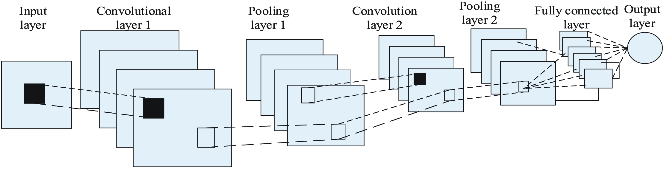
The network structure of the constructed CNN model is shown in Fig. 1, including the input layer, two layers of convolution layers, and two layers of pooling layers. Using grayscale image as input data, the input channel parameter of convolution layer 1 is set to 1, and the output channel parameter is set to 32; the input channel parameter of convolution layer 2 is set to 32, and the output channel parameter is set to 256; fully connected layer input channel. The parameter is set to 256, and the output category is 6 (classification of 6 activities). The size of the convolution kernel in the network is 5 × 5, the size of the pooling layer kernel is 2 × 2, and the step size of the convolution kernel and the pooling kernel is 1.

A.CONVOLUTIONAL LAYER

We use the convolution kernel to convolve the grayscale image input to the convolutional layer, and input the convolution result into an activation function to obtain the feature map after the convolution process. The process is as shown in the following fomulas

u_{j}^{l} = \sum_{i \in s_{i}}^{} x_{i}^{l - 1} \cdot w_{i j}^{l} + v_{j}^{l},

(1)

x_{j}^{l} = f (u_{j}^{l}) .

(2)

where

u_{j}^{l}

represents the activation information output by the j channel of convolutional layer l, where

x_{i}^{l - 1}

represents the input feature map of convolutional layer l, which is the weight coefficient of w_ij convolutional layer l and its upper layer, and

v_{j}^{l}

is paranoid coefficient.

x_{i}^{l}

is the output feature map of convolution layer l, and f is the activation function.

B.POOLING

The convolution layer is conceptually understood as the process and result of the convolution operation, that is, the convolution kernel (parameter matrix) performs convolution calculation on the input data matrix to obtain the feature map. The purpose of the convolution operation is to extract data-related features. The previous convolution layer extracts the low-level features of the data, and the subsequent convolution layer extracts the refined features of the data. Also known as the downsampling layer, it mainly has two functions, feature extraction and dimensionality reduction of the input data. It can ensure that the local characteristics of the input data are unchanged and reduce the dimension of the input data, which is helpful to improve the efficiency of CNN and can effectively prevent the problem of overfitting. Common pooling methods include maximum pooling, random pooling, and average pooling, as shown in

x_{j}^{l} = LS (x_{j}^{l - 1}) .

(3)

where

x_{i}^{l}

is the output feature map of the pooling layer,

x_{j}^{l - 1}

is the input feature map of the pooling layer l, and LS is the pooling function, generally the function of finding the maximum value, random value, and average value. The output results

x_{i}^{l}

of the pooling layer are obtained by pooling convolution kernels to divide several nonoverlapping input feature maps.

C.FULLY CONNECTED LAYER

This layer stitches the 2D feature maps obtained from the previous layers into 1D features as input, and then combines the weight coefficient and bias to use the activation function for classification:

u^{l} = x^{l - 1} \cdot w^{l} + v^{l},

(4)

x^{l} = f (u^{l}) .

(5)

where Unconvertable

u^{l}

represents the static activation information of the fully connected layer l, where

x^{l - 1}

is the feature map output by the previous pooling layer, w^l is the weight coefficient of the fully connected layer, and v^l is the offset. Equation (5) is the classification result of the fully connected layer, the formula f is the activation function, and the Relu function is used in the fully connected layer.

D.DROPOUT LAYER

Disconnect some connections randomly to prevent CNN from overfitting, as shown in Fig. 1, between the fully connected layer and the output layer.

E.OUTPUT LAYER

The eigenvalues output by the fully connected layer get the classification results after the activation function. Generally, the probability of each type is calculated by the soft_max function. The function of the soft_max function layer is to infer the category of behavior, action, or activity, as shown in the following:

C_{r} = s o f t \max (x^{l})

(6)

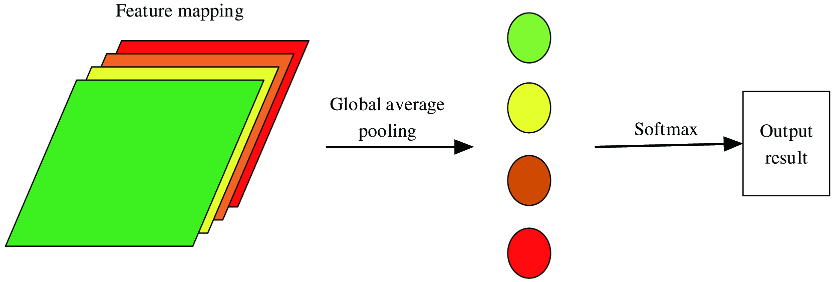
where x^l is the output characteristic of the fully connected layer, and C_r is the classification result.

Pooling is an important operation in CNNs, and its purpose is to reduce the data dimension of convolution output and save computing resources. Commonly used pooling operations are maximum pooling and average pooling. This article uses another constructive strategy, global average pooling, to replace the fully connected layer. Fig. 2 shows the comparison between global average pooling and average pooling used.

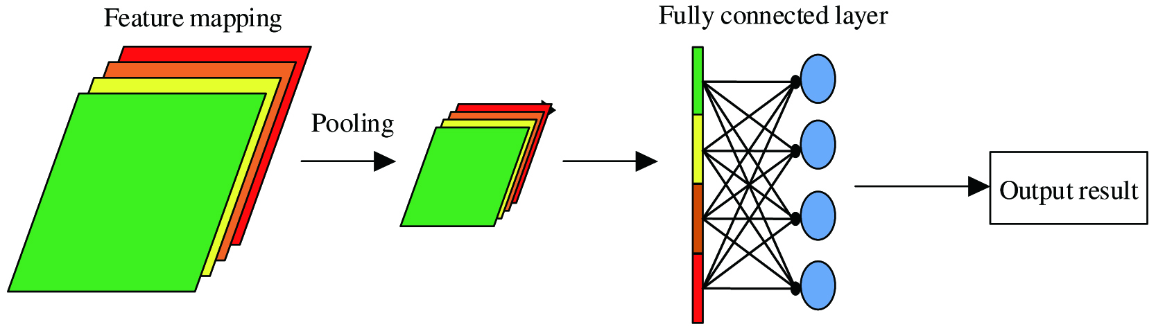Fig. 2. Average pooling and subsequent operations.

It can be seen from Fig. 2 that average pooling reduces the dimensionality of the feature map, and then stretches the reduced feature map into a 1D vector and sends it to the fully connected layer, and finally uses the Soft_max function to output the classification result. However, this method causes many fully connected layer parameters to easily overfit, which affects the generalization ability of the network. The global average pooling used in this article is shown in Fig. 3. That is a pooling window with the same dimension is used to slide on the feature map, and then the pooling result is calculated for average value. The obtained average value composition vector is directly classified using the Soft_max function. The advantage of global average pooling is that it simplifies the structure of the CNN by enhancing the correspondence between the feature map and the fault category. And, it avoids the problem of overfitting and strengthens the credibility of feature map classification.

Fig. 3. Global average pooling and subsequent operations.

III.ALGORITHM IMPLEMENTATION BASED ON CNN

A.STOCHASTIC GRADIENT DESCENT ALGORITHM

Stochastic gradient descent is the most basic and common optimization algorithm in deep learning. The stochastic gradient descent method (SGDM) performs an iterative update through each sample of the training set, so that the cost of improving the overall optimization efficiency is to increase a certain number of iterations and lose a small part of accuracy. In this way, the algorithm will have a relatively large amount of calculation, and every step of the iteration will need to use all the data in the training set, resulting in a long training time. Therefore, the current SGDM generally uses the small batch SGDM. Randomly sample a small batch of randomly distributed samples from the sample. By calculating their gradient mean, you can obtain an unbiased estimate of the gradient. The specific algorithm is shown in Table I.

TABLE I. Stochastic Gradient Descent Algorithm

Require: Learning rate

η

Require: Initial parameters

θ

While The number of iterations does not reach the predetermined number do

A small batch of m samples

{(x^{(1)}, y^{(1)}), \dots, (x^{(m)}, y^{(m)})}

is randomly selected from the training set

Computational gradient estimation:

g \leftarrow \frac{1}{m} \nabla \sum_{i} L (θ; x^{(i)}, y^{(i)})

Parameter update:

θ \leftarrow θ - η g

end while

B.LEARNING RATE CONTROL METHOD

Among the hyperparameters that have a certain impact on the classification accuracy, the learning rate is one of the most important hyperparameters. If the set learning rate is too large, the loss curve may fluctuate or even rise within a certain range. If the set learning rate is too small, it may lead to more iterations of the experiment required. This article uses a learning rate that dynamically changes according to the number of iterations. The learning rate is set to a relatively large value at the beginning of training, so that the accuracy of the model can converge to the ideal state in a short time. However, the loss and accuracy curves may fluctuate significantly. Therefore, the learning rate is reduced in the middle of training, so that the model continues to learn useful information, and the fluctuation range of the curve becomes smaller. In the later stages of training, the learning rate is further reduced, and the fluctuation range of the curve continues to decrease. This method can speed up the training speed of the model, reduce the degree of overfitting, and reduce the number of iterations of the experiment.

The algorithm is divided into three steps:

(1)The previous item calculates the output value $α_{j}$ of each neuron (j represents the jth neuron of the network)
(2)Inversely calculate the error $δ_{j}$ and $δ_{j} = \partial L / \partial I_{j}$ of each neuron (L is the loss function, I_j is the weighted input).
(3)Calculate the gradient of the weight $W_{j i}$ of each neuron ( $W_{j i}$ represents the weight of the connection from neuron i to neuron j) $α_{i} δ_{j} = \partial L / \partial W_{j i}$ . Finally, the weight is updated according to the gradient.

In this section, the step size is 1, the input channel is 1, and the convolution kernel is 1 as a case to derive the CNN reverse learning algorithm. In the CNN, the error is propagated from back to front, and the error

δ^{l}

of the l-th convolutional layer can be calculated from the difference between the expected output and the real output. Next, start calculating the error

δ^{l - 1}

of each neuron in the l-th convolutional layer. In the convolution calculation, there are the following relationships:

I^{l} = conv (W^{l}, a^{l - 1}) + b,

(7)

α^{l} = f (I^{l}),

(8)

where I^l represents the weighted input of the l-th layer, conv() represents the convolution calculation,

W^{l}

represents the convolution kernel of the l-th convolutional layer, a^l-1 represents the output of the G-th layer, b represents the bias, and f() represents the convolutional layer activation function.

According to the chain derivation rule:

δ_{i, j}^{l - 1} = \frac{\partial L}{\partial I_{i, j}^{l - 1}} = \frac{\partial L}{\partial α_{i, j}^{l - 1}} \frac{\partial α_{i, j}^{l - 1}}{\partial I_{i, j}^{l - 1}},

(9)

where

δ_{i, j}^{l - 1}

represents the error of the l-1-th row, the i-th column, and the j-column;

I_{i, j}^{l - 1}

represents the weighted input of the l-1-th layer, the i-th row, and the j-column; and

α_{i, j}^{l - 1}

represents the output of the neuron in the l-1-th row, ith, and jth column. Also,

\frac{\partial L}{\partial α_{i, j}^{l - 1}} = {\sum_{m} \sum_{n} W}_{m, n}^{l} δ_{i + m, j + n}^{l},

(10)

\frac{\partial α_{i, j}^{l - 1}}{\partial I_{i, j}^{l - 1}} = f^{'} (I_{i, j}^{l - 1}) .

(11)

The convolution form is

δ^{l - 1} = W^{l} * δ^{l} ⊙ f^{'} (I^{l - 1}) .

(12)

C.LEARNING RATE CONTROL METHOD

The framework of the CNN-based HAR model designed in this article is shown in Fig. 4. It can be seen from Fig. 4 that the CNN-based recognition model includes model training, model verification, and model testing.

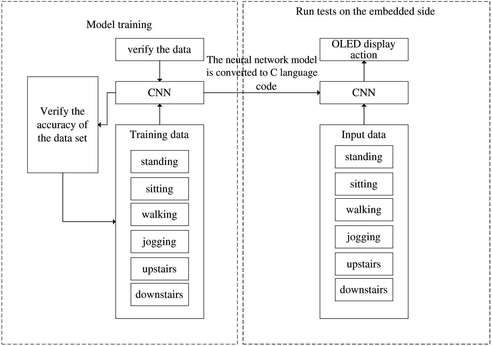Fig. 4. Framework of HAR based on CNN.

As can be seen from Fig. 4, the training and verification of the CNN model is carried out in the training module, and the experimental test is carried out in the testing module. The training module has been trained for many times and uses the validation set data to select the optimal network hyperparameters to obtain the optimal network model. The network hyperparameters selected by the validation set during training include the number of hidden layers and the number of corresponding neurons, the number of convolutional layers, the size of convolution kernels, and the number of convolution kernels. The selection criteria of the optimal model are based on the accuracy of HAR in the test set as the primary indicator.

IV.SYSTEM DESIGN

A.EMBEDDED DEVICE OVERALL ARCHITECTURE

The embedded design structure hierarchy diagram is shown in Fig. 5. The structure hierarchy is mainly composed of the underlying hardware, driver layer, middle layer, and application layer. It mainly includes FreeRTOS (real time operating system) embedded operating system transplantation and Acorn RISC Machine (ARM) processor programming. It uses three-axis accelerometer, to collect human body activity sensor data, and receives commands and data from the host computer through Bluetooth technology.

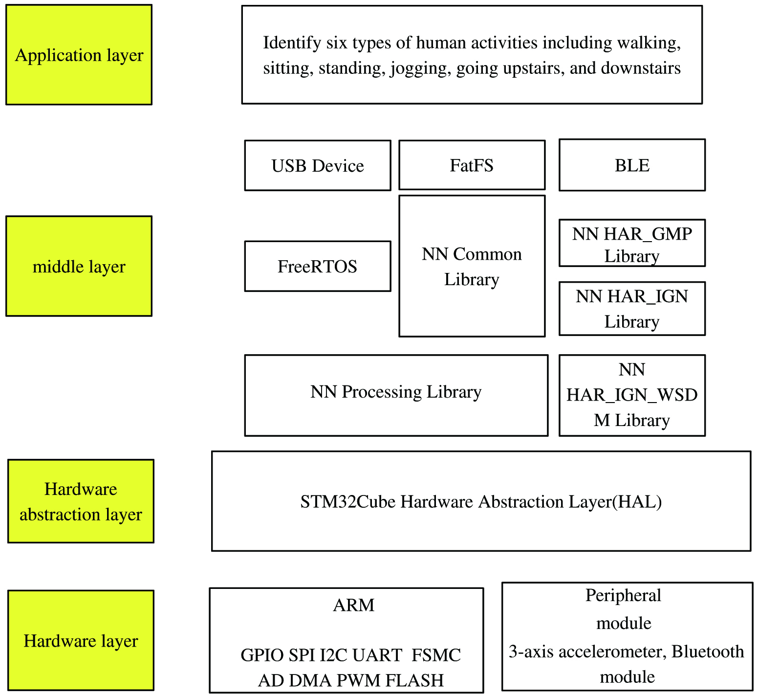Fig. 5. Hierarchical diagram of embedded design structure.

There are many types of sensors that can be used for HAR, and different types of sensors can be selected according to different needs. However, the acceleration sensor is the most widely used sensor in the activity recognition process. Acceleration data are used as the basis of HAR and classification, and the data collected by other sensors provide auxiliary functions, which can cope with more complex application scenarios. The specific functions of the sensors selected for the recognition and classification of human activities are as follows:

(1)Acceleration sensor: This sensor is highly sensitive to tiny vibrations and is very suitable for recording state changes during human activity. The collected acceleration data are used as the main basis for HAR.
(2)Air pressure sensor: This sensor is mainly used to determine whether the human body is performing behavior activities that change in height, such as going up and down stairs. When a person is climibing up the stairs, the value collected by the barometer will become smaller, and when the person is going down the stairs, the value collected by the barometer will become larger.
(3)Orientation sensor: As like inertial navigation sensor, this kind of sensor is mainly used for determining whether the user has changed the direction while walking or running.
(4)It has the function of wireless transmission: the system hardware should be equipped with wireless transmission modules, such as Bluetooth, Wi-Fi, and other modules. The collected data or the results of identification and classification can be transmitted to the remote server for further processing and analysis using the wireless module.

B.SYSTEM CPU

The STM32F767 from STMicroelectronics was selected as the system CPU. The reasons for the selection are as follows:

(1)The core based on Cortex-M7 is equipped with digital signal process (DSP) instructions and the DSP library launched by ARM, so that the chip calculation speed can be improved, and the calculation speed of neural network on the chip can be realized.
(2)With low power consumption mode, CPU uses high-speed clock (HCLK) to provide clock and execute program code to reduce system power consumption.
(3)With up to 1 Mb of flash memory; 1024 bytes of OTP memory; SRAM: 320 Kb (including 64 Kb data TCM RAM to save critical real-time data), 16 Kb instruction TCM RAM (save critical real-time program), and 4 Kb backup SRAM (using ultralow power consumption mode); flexible external memory controller with up to 32-bit data bus: SRAM and SDRAM memory.

Based on the above three points, it can meet the needs of system design.

C.DATA ACQUISITION SENSOR

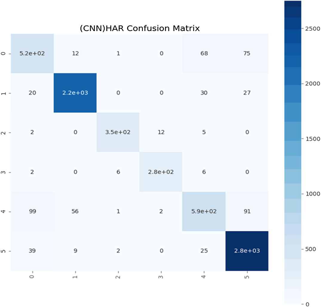
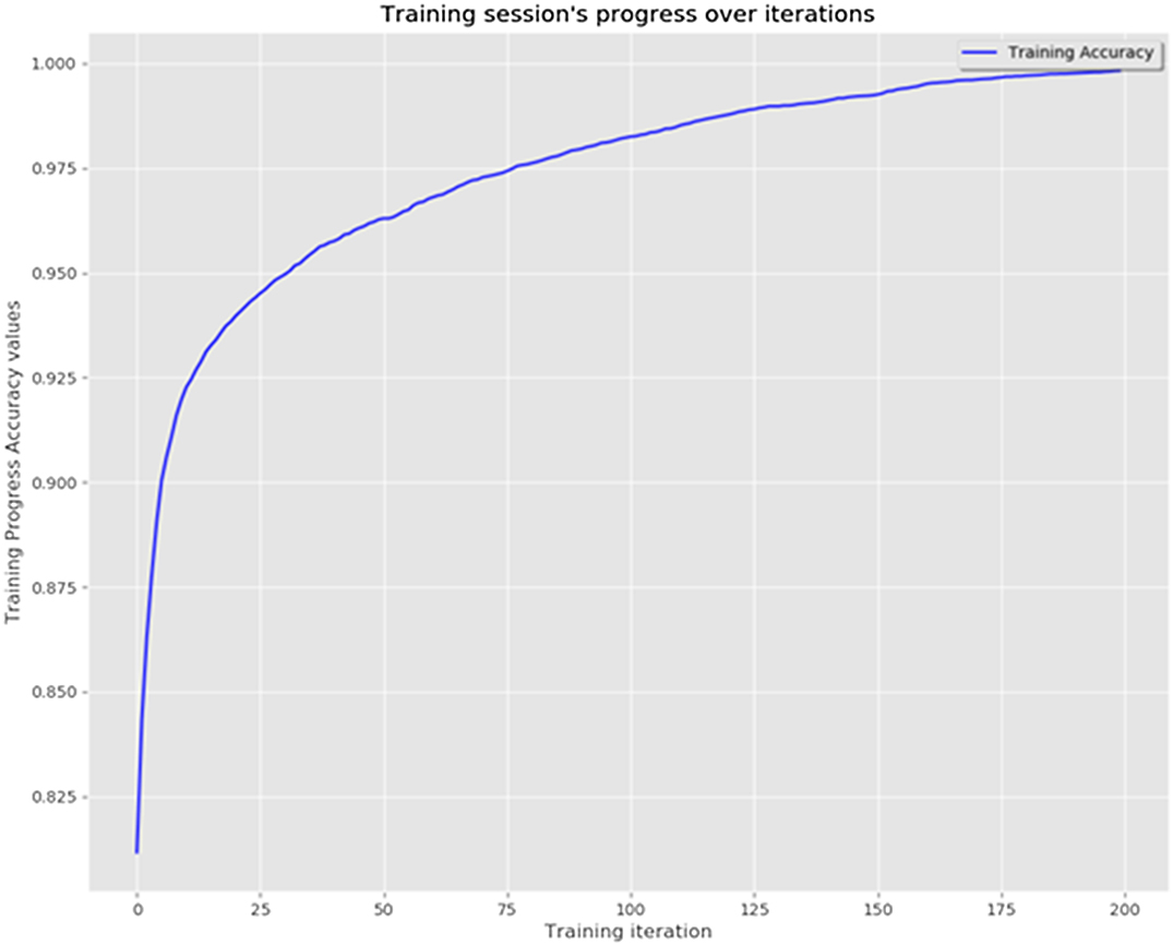
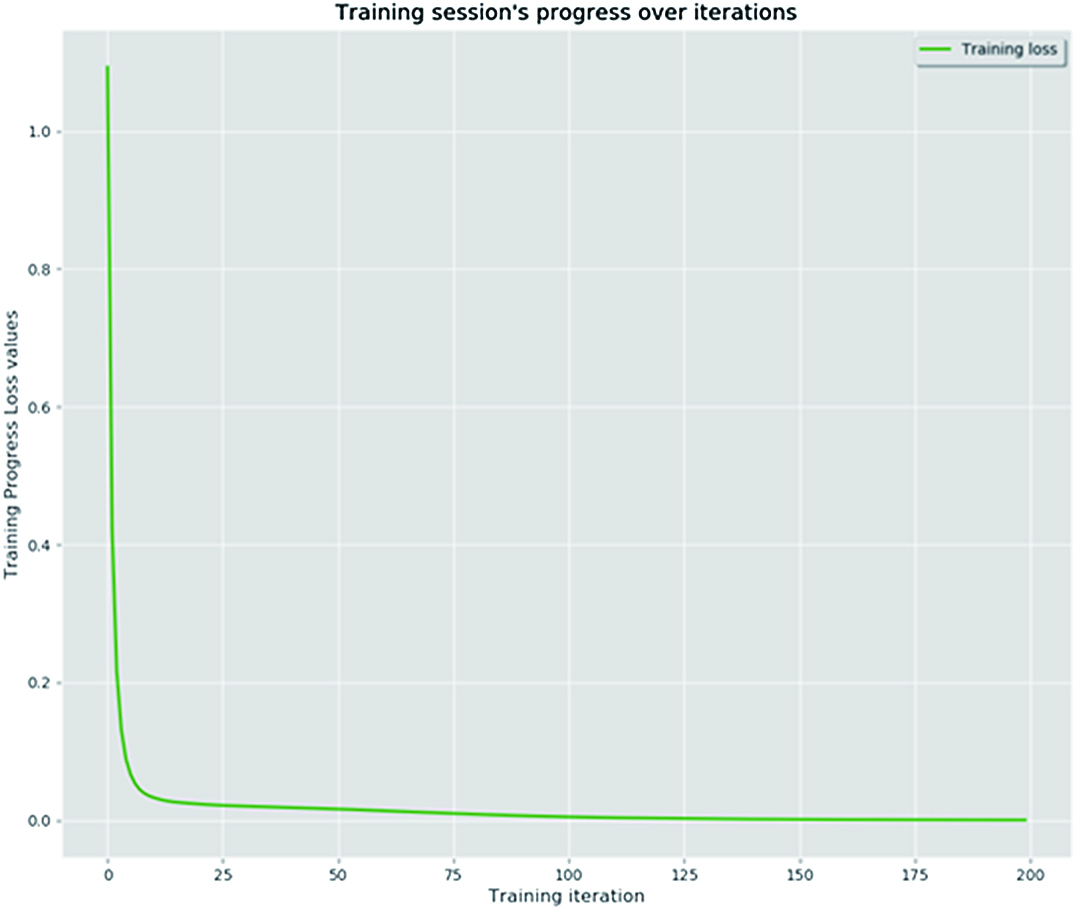
Figs. 6–11 are data visualization diagrams corresponding to six kinds of actions, respectively, shows the activity curve of the acceleration data of the x, y, z axes of 6 activities. Fig. 12 shows a schematic diagram of the process of loading the convolutional neural network onto the STM32 microcontroller. After the C code is generated by the STM32CubeMX tool, the final model is run on the microcontroller and displayed in real time on the OLED screen. Fig. 13 shows that the model generated by the convolutional neural network draws the confusion matrix diagram of the recognition rate of the six activities. The values 0–5 represent the six specific human activities of standing, sitting, walking, jogging, going up stairs, and going down stairs. Fig. 14 shows the accuracy function graph when training the convolutional neural network model. It can be seen that the recognition rate of the final model training is 94.2%.

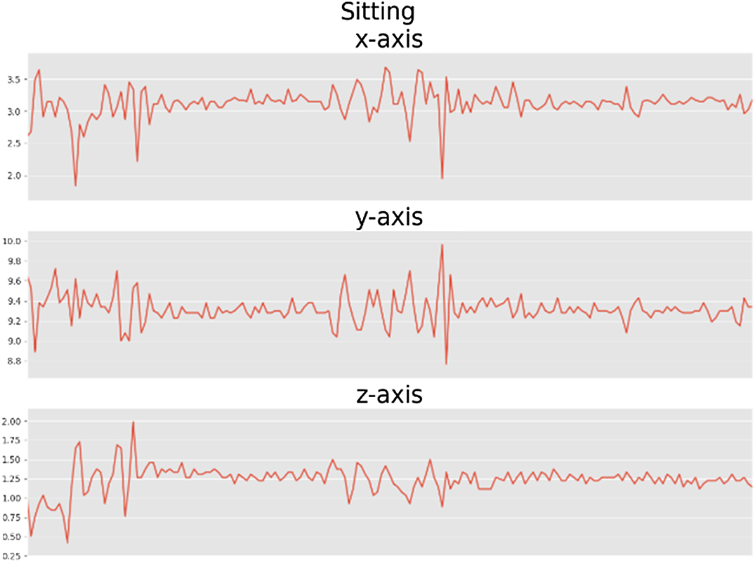Fig. 6. Sitting x-axis, y-axis, and z-axis analysis chart.

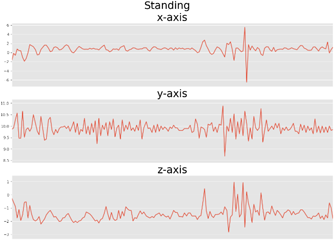Fig. 7. Standing x-axis, y-axis, and z-axis analysis chart.

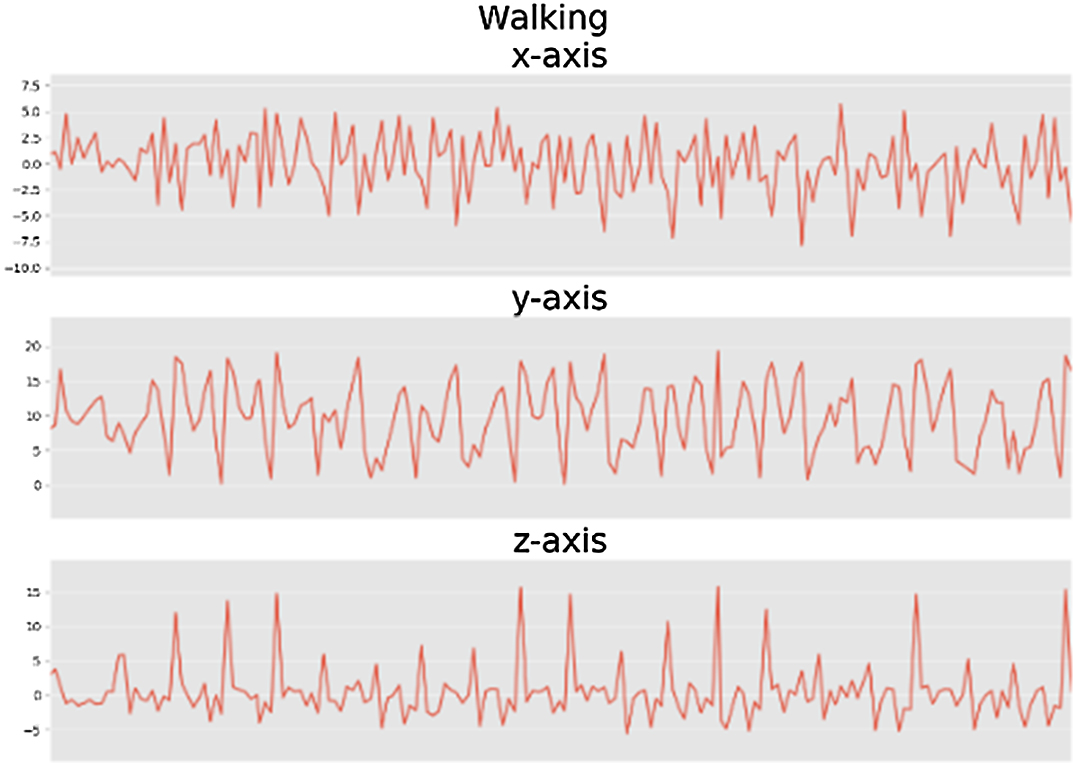Fig. 8. Walking x-axis, y-axis, and z-axis analysis chart.

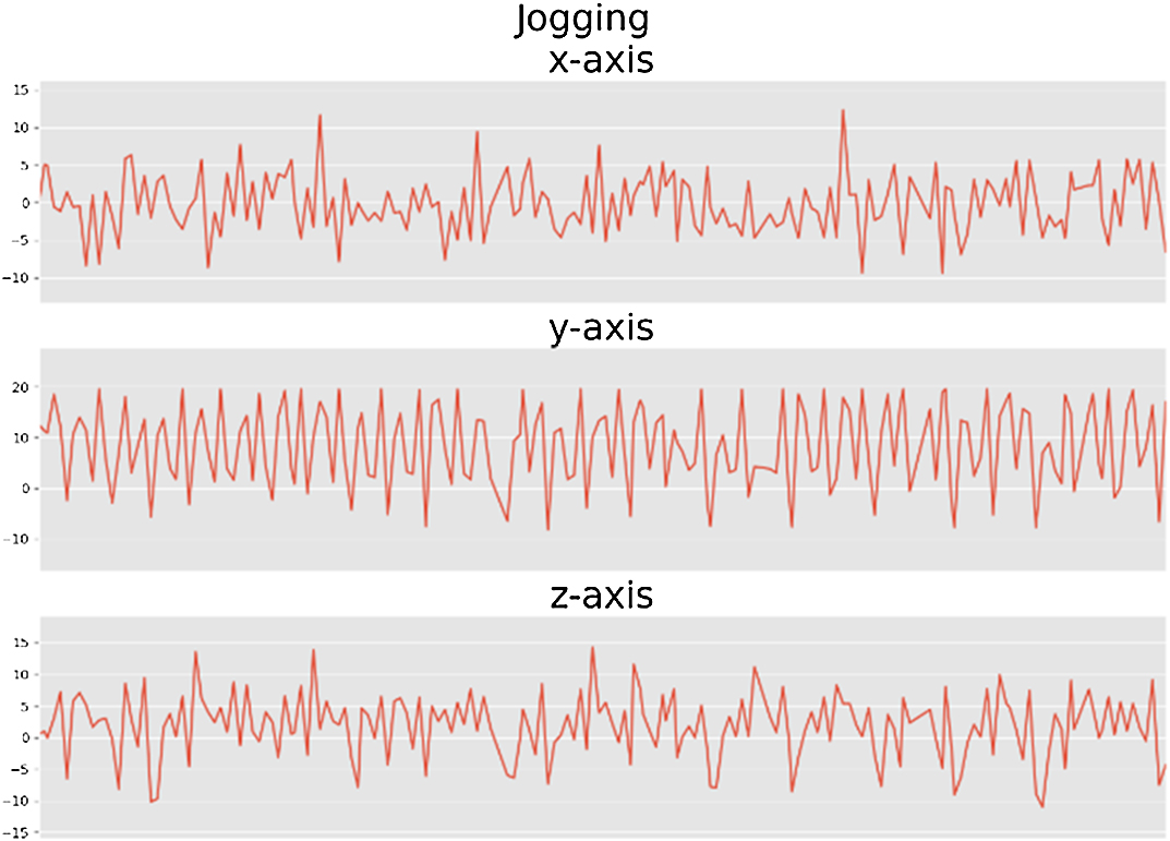Fig. 9. Jogging x-axis, y-axis, and z-axis analysis chart

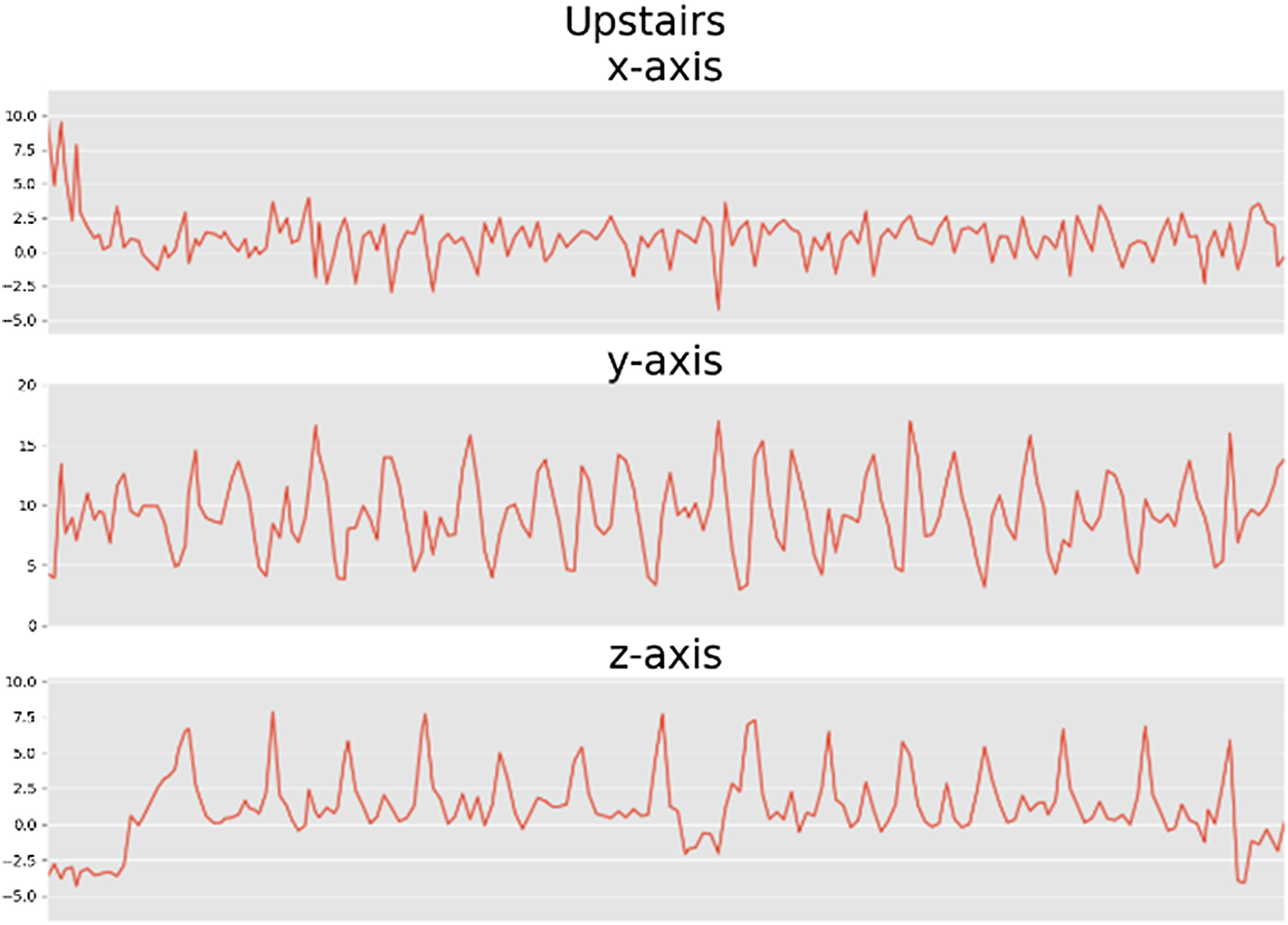Fig. 10. Upstairs x-axis, y-axis, and z-axis analysis chart.

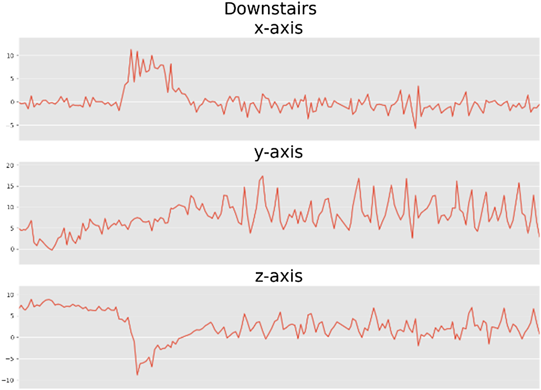Fig. 11. Downstairs x-axis, y-axis, and z-axis analysis chart.

An acceleration sensor is a sensor that can measure acceleration. It is usually composed of mass, damper, elastic element, sensitive element, and adaptive circuit. During the acceleration process, the sensor uses Newton’s second law to obtain the acceleration value by measuring the inertial force of the mass. The acceleration sensor used in this subject is MPU-6050. The accelerometer’s measurable range is ±2, ±4, ±8, and ±16g. An on-chip 1024-byte first input first output (FIFO) helps reduce system power consumption. Communication with all device registers uses 400 kHz I2C interface. For applications that require high-speed transmission, 20 MHz serial peripheral interface (SPI) is available for reading and interrupting registers. In addition, a temperature sensor and an oscillator with only ±1% variation in the working environment are embedded on the chip. The chip size is 4 × 4 × 0.9 mm, using QFN package (leadless square package), which can withstand a maximum impact of 10,000 g, and has a programmable low-pass filter. Regarding power supply, MPU-6050 can support VDD range 2.5 V ±5%, 3.0 V ±5%, or 3.3 V ±5%.

D.OVERALL SOFTWARE DESIGN PROCESS

We use STM32F767 to collect sensor data, input the data collected by the sensor into the CNN, train the CNN on the PC side (operating in Python3.6.3 and Tensorflow1.6.0 environment), and pass the trained convolutional nerve through the cube. AI in the CUBEMX software is compressed four times and then loaded onto the embedded system. At the embedded end, the data from the acceleration sensor are input to the CNN. The CNN automatically detects the human body movements and displays the current status through the organic light-emitting diode (OLED) screen.

V.EXPERIMENTAL RESULTS AND ANALYSIS

The experimental environment used in this article is PC-side operating system Windows, graphics card NVIDIA GeForce GTX 1080, programming language Python 3.5; the development software used is Pycharm, the Keras deep-learning framework, and the back end is TensorFlow. The embedded software is STM32CubeMX-AI with the programming language C.

In the experiment, the stochastic gradient descent algorithm is used to train the activity recognition model. A tenfold cross-validation method was used to evaluate the proposed method. If the number of experimental iterations is less than 375, set the learning rate to 0.005. If the number of experimental iterations exceeds 375, the learning rate is set to 0.001. Table II shows the parameter values of the experimental settings.

TABLE II. Stochastic Gradient Descent Algorithm

Parameter	Value
Input vector size	90
Filter value	60
Pooled size	3 × 3
Dropout	0.75
momentum	0.9
Weight decay	0.0001
Mini batches	10
The maximum number of iterations	200
Activation function	ReLU

In this experiment, the network architecture and hyperparameter settings are: two CNN layers, each of which includes a convolutional layer, a batch normalization layer, a modified rectified linear unit (ReLU) activation function layer, and a maximum pooling layer. After two such CNN layers, a fully connected layer and a Soft_Max function layer are used to give the final classification results. In addition, the mini-batch size is set to 100, and the initial learning rate of the CNN network is set is 0.001. We added a validation set to the experimental plan. For the convenience of the experiment, the experimental sample data were expanded. The specific method is to expand the 89,670 training data samples to 10,000 in the form of random replication, and we will also randomly expand the 2947 test data samples to 3000. At the same time, we use the SGDM to optimize the parameters of the experiment, and the maximum number of iterations of the experiment is set to 200.

A.EMBEDDED DEVICE OVERALL ARCHITECTURE

In this work, the training dataset uses STM32F767CPU to collect six types of activity data, each with 10,000 groups, a total of 68,572 groups of data. In order to make the results more convincing, we used the public dataset in the wireless sensor data mining (WISDM) database to test the model we trained; WISDM dataset is used to test the method proposed in this article. The dataset has a total of 1,098,213 samples, which come from 29 users. The experimental dataset includes six activities: walking, sitting, standing, jogging, going upstairs, and going downstairs. The sampling rate is 20 Hz.

The collected sensor signal is preprocessed by a noise filter, and then sampled in a sliding window with a fixed width of 2.56 s. The overlap rate is 50%, that is, the amount of data in each window is 128. We assume that gravity has only low-frequency components. Therefore, a Butterworth low-pass filter with a cutoff frequency of 0.3 Hz is used to divide the acceleration signal of the sensor into a gravitational acceleration signal component and a linear acceleration signal component. There are 7352 training data and 2947 test data in the dataset. For the convenience of calculation, we randomly expand the training samples to 8000, and then randomly select 1000 samples from these 8000 training samples as the verification set required for the experiment; similarly, we randomly expand the 2947 test samples to 3000. It can be seen from previous studies that frequency domain data are more effective than time domain data for HAR. Therefore, only frequency domain data are used in our experimental scheme 1. More specifically, the result of the FFT of the input data is used as the input of the network.

The confusion matrix is a table describing the performance of the classifier/classification model. It contains information about the actual and predicted classification performed by the classifier, and this information is used to evaluate the performance of the classifier.

From the CNN_Matrix confusion matrix map, 0 means downstairs, 1 means jogging, 3 means standing, 4 means upstairs, and 5 means walking. The diagonal left is the correct data; it can be seen that the training effect has reached the expected value.

This article searches for the optimal CNN network model as follows:

(1)Select N (initial N = 2) convolutional layers, perform training, save the model, and calculate the average accuracy of the test set; increase the number of pooling layers, continue training, save the model, and calculate the average accuracy of the test set. When the average accuracy of the test set of the model drops twice in a row, stop training; take the model with the highest average accuracy of the test set as the best model in this group of experiments, and obtain the K-th (initial K = 1) optimal model.
(2)Increase the number of convolutional layers, that is, N = N + 1, repeat step (1), K = K + 1.
(3)When the average accuracy of the test set of the best model obtained drops twice in a row, stop the experiment.
(4)Compare the average accuracy of the test set of the best model obtained in each group of experiments, and select the best model.

The loss of the training set in the training of the CNN model changes with the number of training as shown in Fig. 15. As the number of iterations increases, the loss function gradually becomes smaller.

Fig. 12. System flow chart.

Fig. 13. CNN_Matrix confusion matrix map.

Fig. 14. CNN test results.

Fig. 15. Loss function graph.

B.COMPARISON OF EXPERIMENTAL RESULTS

Five testers were selected and performed three experiments. The test method is to fix the embedded device on the waist and make corresponding movements. For the convenience of recording and subsequent analysis, the testers will perform the same movement continuously for 60 s to complete one after the action, do the next action (including sitting, standing, jogging, walking, upstairs, and downstairs). After all the six actions are completed, they are recorded as a set of tests. The test results are printed on the OLED screen in real time, and the action results are sent to the mobile phone through the Bluetooth serial port for subsequent analysis. The result is output every 2 s according to the activity period. Therefore, each person will have 180 action tag data stored in the SD card for each test. The final recognition accuracy is calculated according to the correct number of samples divided by the total number of samples.

Table III shows the final recognition rates of the three machine learning models. It can be seen that the CNN model has the best recognition effect, reaching 94.2%.

TABLE III. Comparison of Results Between Traditional Recognition Methods and CNN Recognition Algorithms

Recognition algorithm	J48	SVM	CNN
Recognition rate (%)	50.8	62.3	94.2

VI.CONCLUSION AND OUTLOOK

This article uses the CNN algorithm to train the neural network model and adds the stochastic gradient descent algorithm to optimize the model parameters and recognize the six behaviors of walking, sitting, standing, jogging, upstairs, and downstairs. Classification and experiments prove that compared with the traditional manual feature extraction method, the CNN model designed in this article has a recognition rate of 94.2% for human activities.

At present, although the research on HAR based on wearable sensors has achieved good experimental results and the classification accuracy is satisfactory, there are still the following problems worthy of further research.

First, wearable devices are used casually in daily life. However, the current algorithms are closely related to the location and method of device placement. And can effectively distinguish various behaviors and activities, it is still one of the current research hotspots and difficulties. Second, the human body’s daily behaviors and activities are complex and diverse. At present, HAR is mostly focused on the recognition of simple activities, such as walking, running, up and down stairs, etc. How to combine contextual information (e.g., Global Positioning System information) for higher semantics behavioral recognition is also a direction to be studied.

Human Activity Recognition and Embedded Application Based on Convolutional Neural Network

I.INTRODUCTION

II.CNN ALGORITHM

A.CONVOLUTIONAL LAYER

B.POOLING

C.FULLY CONNECTED LAYER

D.DROPOUT LAYER

E.OUTPUT LAYER

III.ALGORITHM IMPLEMENTATION BASED ON CNN

A.STOCHASTIC GRADIENT DESCENT ALGORITHM

B.LEARNING RATE CONTROL METHOD

C.LEARNING RATE CONTROL METHOD

IV.SYSTEM DESIGN

A.EMBEDDED DEVICE OVERALL ARCHITECTURE

B.SYSTEM CPU

C.DATA ACQUISITION SENSOR

D.OVERALL SOFTWARE DESIGN PROCESS

V.EXPERIMENTAL RESULTS AND ANALYSIS

A.EMBEDDED DEVICE OVERALL ARCHITECTURE

B.COMPARISON OF EXPERIMENTAL RESULTS

VI.CONCLUSION AND OUTLOOK

REFERENCES