I.INTRODUCTION
Quantum computing is a multidisciplinary field that builds on quantum mechanics, linear algebra, computer science, and several other related fields. On the other hand, it provides contributions back to these fields and others. In order to provide a baseline for the discussions in this work, this section will provide an introductory overview of gate-model quantum computing, one of the most popular methods for quantum programming [1]. The fundamental unit of quantum computing, the qubit, can be represented as a vector in a complex number Hilbert space. Each entry of the vector is the amplitude for that result, corresponding to the probability of measuring that result. For example, a two-qubit system with vector entries [, 0, 0, ] corresponds to a qubit that, when measured, has a 50% chance of measuring 00 and a 50% chance of measuring 11. This system is in a superposition (i.e., the system is in multiple states until measured, and the result is randomly determined according to the probability amplitudes) and the two qubits in this system are entangled (i.e., the result of measuring one of the qubits is directly correlated with the result of measuring the other). These concepts of superposition and entanglement form the foundation for many of the advantages provided by quantum computing [1].
These systems can be programmed by applying gate operations to the qubits. Gates can be viewed as matrices and the application of these gates as the multiplication of the gate and the vector. In order for a matrix to be eligible as a gate, it must be unitary, meaning that the product of a matrix and its complex conjugate transposed must be the identity matrix. The result of this condition is that all quantum gate operations are reversible, unlike classical gate operations (e.g., AND gate) [1]. To perform quantum programming, a variety of languages and libraries are available. One popular library is Qiskit, which offers direct support for IBM’s cloud-based quantum computers as well as several simulators [2]. Multiple frontend interfaces exist for Qiskit, including the Qiskit Python library and IBM’s Quantum Composer. The Visual IoT/Robotics Programming Language Environment (VIPLE) [3] also offers a simple visual interface to Qiskit.
VIPLE is an open standard and free programming language widely used in teaching computer science, programming, parallel processes, service-oriented computing, and artificial intelligence [4,5]. Fig. 1 shows the Basic Activities that perform basic computation tasks, Quantum Basic Activities, and Quantum Services of VIPLE that perform quantum-related operations. These activities and services can be dragged and dropped into the code area to form workflows of code. VIPLE will be used to facilitate the illustration of a simple quantum program in this paper, as it eliminates most of the overhead, especially in simple circuits. In practical applications, the use of VIPLE provides multiple other benefits, such as strong support for concurrent, IoT, robotics applications, as well as an AI-based autograder and tester [6,7].
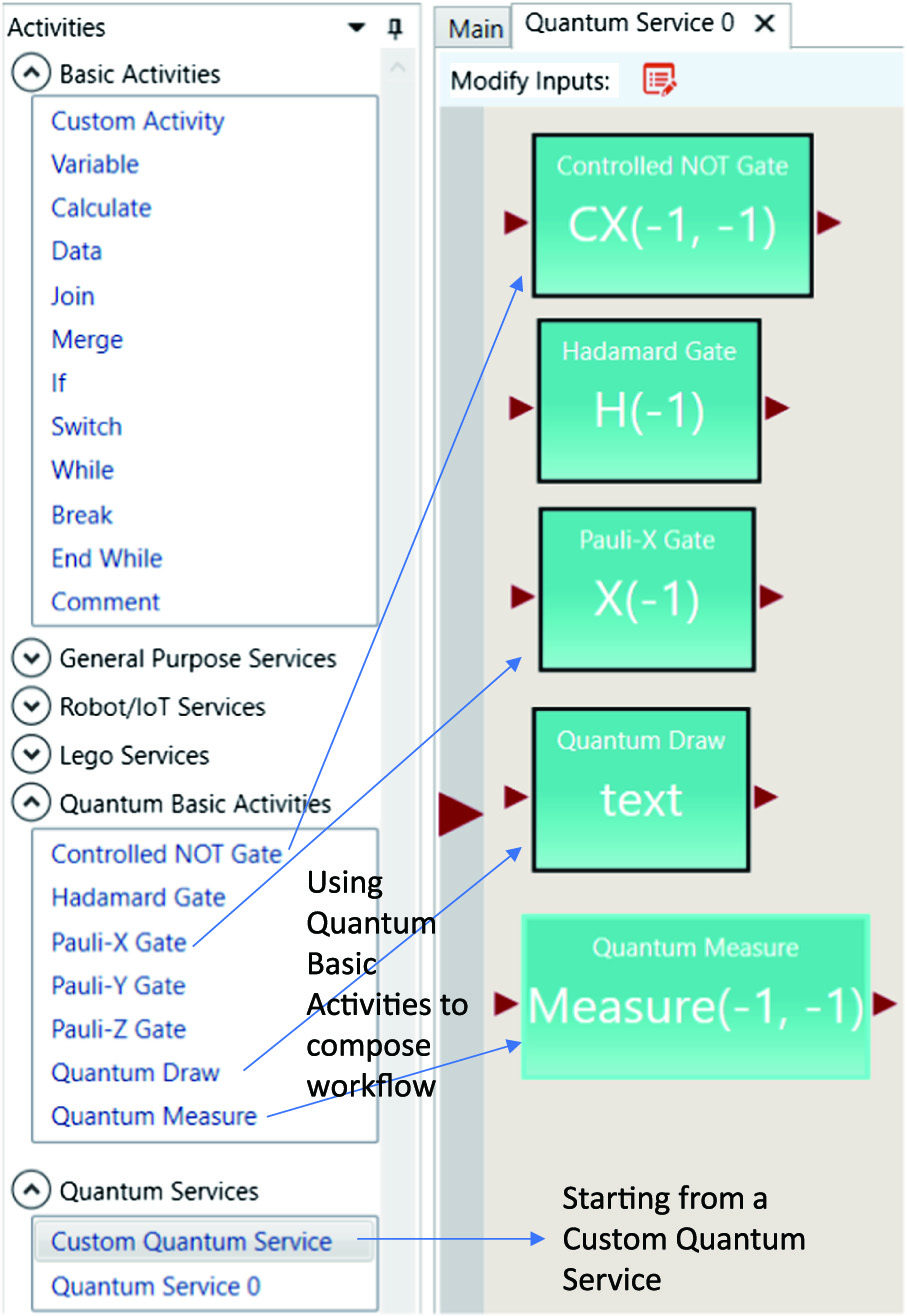 Fig. 1. Using VIPLE activities and services.
In this example, a two-qubit system is created. By default, the state of each qubit defaults to , leaving the system initially in the state , or in vector form, [0,0,0,1]. The Hadamard gate (H) is first applied to qubit 0, and then a controlled not gate (CX) is applied to qubits 0 and 1. To apply the single-qubit Hadamard gate to this two-qubit system, a new matrix needs to be calculated using the tensor product operation. In this case, the first matrix would be I⊗H (or H⊗I depending on qubit ordering) [1,2] and the second matrix is CX as the controlled not gate is already a two-qubit gate. Fig. 2 shows the VIPLE code for this circuit.
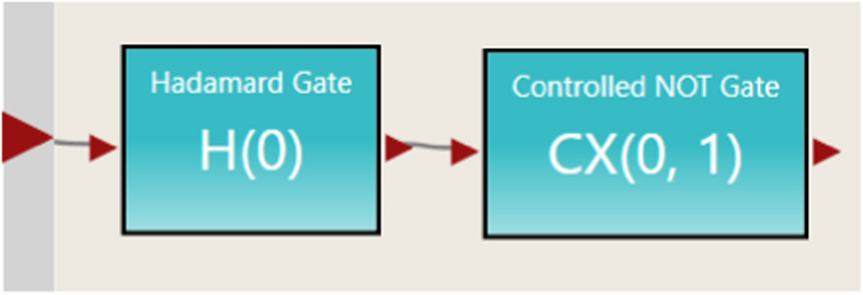 Fig. 2. VIPLE quantum circuit.
Using Qiskit’s draw function, the circuit created in VIPLE can be visualized, as shown in Fig. 3. Notably, the connection between qubits 0 and 1 by the controlled not gate can be clearly seen. This coordination between the values of qubits is a vital component of quantum programming and enables the creation of entangled states.
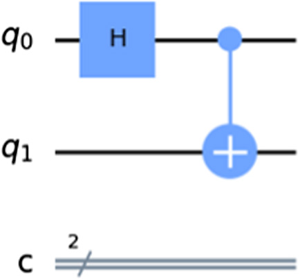 Fig. 3. Qiskit drawing of VIPLE circuit.
VIPLE enables a quantum circuit to output either the amplitudes of the circuit or the value of the classical bits. Instead of measuring the result and outputting the (random) classical bit result, this example outputs the probability amplitudes, as shown in Fig. 4. This state is equivalent to the example from the introduction, [, 0, 0, ]. Notably, this is a Bell state (also known as an EPR pair) [1] and is in an even superposition between and , where the two qubits are entangled together.
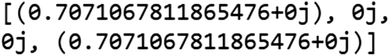 Fig. 4. Amplitudes of VIPLE circuit.
In the following sections, we will survey the current research on applications of quantum computing to machine learning and discuss future directions in the field. Specifically, we will look at applications of hybrid quantum-classical (HQC) systems to quantum machine learning (QML) on noisy intermediate-scale quantum (NISQ) era systems.
QML provides opportunities for several key advantages over classical models. These potential advantages include a speedup in training time, an increase in accuracy over classical approaches, and the ability to directly model quantum mechanical systems, among other advantages. With the limitations of the NISQ era, these advantages are more difficult to achieve and require additional research to better leverage these quantum systems. A primary goal of this survey paper is to detail some of the modern approaches to help further research in these areas.
The remainder of the paper is organized as follows. Section II provides an introduction to NISQ era quantum computing. Section III discusses fundamentals of QML. Section IV showcases applications of QML to classification tasks. Section V discusses the barren plateau problem. Section VI explores solutions to improve QML accuracy and performance. Section VII provides examples of quantum convolutional neural networks (QCNNs). Section VIII concludes the paper.
II.NISQ ERA
Advances in quantum computing have led to the NISQ era. Physical quantum computers with upwards of hundreds of qubits are available. Certain quantum computers are also available as cloud services, such as IBM’s quantum computers [2]. These NISQ era quantum computers are noisy, meaning that the quantum states lack stability. As time progresses, the states decohere, resulting in a loss of accuracy. Furthermore, the gates used to manipulate the qubits often create slight deviations, resulting in incorrect solutions [8]. Despite these issues, the realization of such machines enables the implementation of a certain subclass of quantum and HQC algorithms. In order to successfully implement these algorithms, several considerations must be made during the implementation and testing processes. Several such considerations include how data are encoded in qubits (e.g., binary encoding or amplitude encoding) and how oracles are implemented (e.g., how many ancilla qubits are needed and how many gates are required to implement the required functionality) [8].
A physical shortcoming of these devices is the connectivity of the qubits. In some cases, qubits are not fully connected, which can result in problems if disconnected qubits are needed for one operation. For example, the CNOT gate is often used to entangle two qubits together. If the two qubits are not physically connected, SWAP gates must be used to perform the operation. However, the use of extra gates increases the time taken and decreases the accuracy of the results [8]. Various other issues such as readout errors and differences in architecture between different quantum computers also contribute to the inaccuracy of NISQ era quantum computers [8].
Future research on NISQ era programming ranges from potential algorithms to error correction. There are many such classes of algorithms that have been explored, such as machine learning, combinatorial optimization, and numerical solvers. These classes include subclasses such as supervised and unsupervised learning, reinforcement learning, the max-cut problem, singular value decomposition, and quantum error correction (QEC) [9].
Quantum computing offers a platform for addressing many modern computing problems with a potential for better space and time complexity as a result of quantum concepts such as superposition and entanglement. Within the area of machine learning alone, many different approaches have been proposed to provide speedup to various algorithms. Some such algorithms are Bayesian inference, Boltzmann machines, principal component analysis, support vector machines, and reinforcement learning [10]. Speedups have been observed ranging from O(log n) to O(√(n)). However, quantum computers with sufficiently many qubits and error correction do not yet exist. As such, the applicability of these approaches on NISQ era quantum computers should be explored. Specifically, factors such as number of gates, information encoding, and error handling are greatly impacted by the use of NISQ era quantum computers [8].
In the next sections, we will explore applications of NISQ era quantum computing to QML.
III.QML FUNDAMENTALS
One approach to developing machine learning algorithms on NISQ era quantum computers is through the use of HQC algorithms. Such algorithms typically make use of parameterized quantum circuits (PQCs), which are quantum gates whose effects are dependent on the chosen parameter. Such gates may be rotational gates (e.g., x, y, or z) with the rotation angle serving as the parameter. These gates are unitary operations and are applied to some reference state. In conjunction with these PQCs, entanglement is often applied using, for example, CNOT gates. In this way, the power of entanglement can be leveraged, offering potential for greater accuracy and nonlinearity [11].
By introducing parameterization to quantum circuits in this way, external classical algorithms can control the way in which unitary operations are applied, thereby enabling training of the quantum algorithm through classical means. Thus, PQCs act as a point of contact between quantum and classical systems in HQC applications. PQCs are analogous to classical neurons, in that the parameters act as the weights and biases do for the classical neuron. As such, PQCs can serve as the foundation for various HQC applications such as HQC machine learning [11]. This paper will explore such applications.
In order to reason about the efficacy and state of these quantum circuits, mathematical definitions for various features of circuits have been provided. Three such major features are expressibility, entangling capacity, and circuit cost. By calculating these values, different applications of PQCs and entangling gates can be compared to provide information about the strength of various approaches in different applications.
Expressibility is the ability of a circuit to generate pure states that are well representative of the Hilbert space. In order to calculate the expressibility of such states, Haar random states are employed. Specifically, the state fidelities generated by the sample ensemble of parameterized states are compared to the ensemble of Haar random states. In this way, the distributions of representations of the Hilbert space can be directly computed and compared [11].
Entangling capacity is calculated by employing the Meyer–Wallach entanglement measure. This measure specifies how entangled a system is. If the circuit is composed of only product states (i.e., no entanglement), the entangling capacity is 0. The more entangled the circuit is, the closer this value will be to 1 [11]. The Meyer–Wallach measure has various other applications as well, such as tracking the convergence of pseudorandom circuits by computing the deviation of the Meyer–Wallach measure from the Haar value [11].
Circuit cost, or the cost of implementing the circuit, is measured according to the circuit depth, circuit connectivity, number of parameters, and number of two-qubit gates [11]. As discussed in the previous section, increasing the number of gates in NISQ era quantum computers can further decrease the accuracy and reliability of the results. As such, circuit cost should be minimized when possible. However, there is typically a tradeoff between circuit cost and expressibility, up to a certain point. Such comparisons have been experimentally explored for various types of circuits, demonstrating this tradeoff [11].
The introduction of PQCs offers hope for the capability of quantum programs to provide a new platform for various machine learning algorithms. Such capability has been both experimentally and theoretically demonstrated using a single qubit. Specifically, the combination of a single qubit with data re-uploading and a classical subroutine ‘[provide] sufficient computational capabilities to construct a universal quantum classifier [12].’ This demonstration provides a foundation for performing machine learning with HQC algorithms by employing PQCs.
To demonstrate some of the features of qubits for machine learning, a circle classification task was performed. Specifically, various points were randomly generated on a plane and labeled according to whether they were inside or outside a circle of radius r. This problem highlights the strength of qubits for problems involving circles. Specifically, qubits are likely well-suited to this task because gates are rotational in their behavior. A single-qubit network achieved 94% accuracy with only 2 layers (12 learnable parameters). A two-qubit network achieved 96% accuracy with 2 layers (22 learnable parameters). With the addition of a second qubit, entanglement can be employed. However, the results in this example were unaffected by entanglement. With the addition of more layers, entanglement offered very little effect, varying according to number of layers, but no more than 2% difference (e.g., 97% instead of 95%). With a four-qubit network, 96% is once again achieved using 2 layers (42 parameters) [12]. The detailed results from this experiment are shown in Table I. The first row lists the number of qubits. Non-entangled qubits are labeled ‘No Ent.’ and entangled qubits are labeled ‘Ent.’ The results correspond to the success rate.
TABLE I. Circle classification [12]
| Qubits Layers | 1 | 2 No Ent. | 2 Ent. | 4 No Ent. | 4 Ent. |
|---|---|---|---|---|---|
| 1 | 0.50 | 0.76 | – | 0.76 | – |
| 2 | 0.94 | 0.96 | 0.96 | 0.96 | 0.96 |
| 3 | 0.94 | 0.97 | 0.95 | 0.97 | 0.96 |
| 4 | 0.94 | 0.97 | 0.96 | 0.97 | 0.96 |
| 5 | 0.96 | 0.96 | 0.96 | 0.96 | 0.96 |
| 6 | 0.95 | 0.96 | 0.96 | 0.96 | 0.96 |
| 8 | 0.97 | 0.95 | 0.97 | 0.95 | 0.96 |
| 10 | 0.96 | 0.96 | 0.96 | 0.96 | 0.97 |
A second experiment was performed using three circles instead of one. For applications involving multiclass classification, the potential for local minima creates potential inaccuracy. Furthermore, the presence of local minima implies that increasing the number of qubits or number of layers does not necessarily increase accuracy. In this case, a single-qubit network required 10 layers (54 learnable parameters) to achieve the maximum single qubit accuracy, 92%. However, this problem offers greater potential improvements through the use of entanglement. A noticeable example is in the two-qubit network case. With four layers and no entanglement, 84% accuracy is achieved. Introducing entanglement increases the accuracy to 91% [12]. The results for this experiment are shown in Table II. The headings are identical to those from Table I.
TABLE II. Three circles classification [12]
| Qubits Layers | 1 | 2 No Ent. | 2 Ent. | 4 No Ent. | 4 Ent. |
|---|---|---|---|---|---|
| 1 | 0.75 | 0.81 | – | 0.88 | – |
| 2 | 0.76 | 0.90 | 0.83 | 0.90 | 0.89 |
| 3 | 0.78 | 0.88 | 0.89 | 0.90 | 0.89 |
| 4 | 0.86 | 0.84 | 0.91 | 0.90 | 0.90 |
| 5 | 0.88 | 0.87 | 0.89 | 0.88 | 0.92 |
| 6 | 0.85 | 0.88 | 0.89 | 0.89 | 0.90 |
| 8 | 0.89 | 0.91 | 0.90 | 0.88 | 0.91 |
| 10 | 0.92 | 0.90 | 0.91 | 0.87 | 0.91 |
As these circle problems suggest, certain problems are better suited to quantum classifiers, whereas other problems still achieve higher accuracy through classical classifiers, such as neural networks (NNs) or support vector classification (SVC). In the following examples, the results for the quantum classifier are defined by the fidelity cost function with single-qubit classifiers with no more than 10 layers. As such, the results for these examples are better suited for comparison but may vary slightly from the aforementioned results. For example, the three circles problem achieves 88% accuracy with a NN, 66% with a SVC, and 91% with the quantum classifier. A non-convex shape achieves 99% accuracy with a NN, 77% with a SVC, and 96% with a quantum classifier [12]. The full results are shown in Table III. The fidelity cost function results are labeled χ2f and the weighted fidelity cost function results are labeled χ2wf.
TABLE III. Quantum/classical comparison [12]
| Classical | Quantum | |||
|---|---|---|---|---|
| Problem | NN | SVC | χ2f | χ2wf |
| Circle | 0.96 | 0.97 | 0.96 | 0.97 |
| 3 Circles | 0.88 | 0.66 | 0.91 | 0.91 |
| Hypersphere | 0.98 | 0.95 | 0.91 | 0.98 |
| Annulus | 0.96 | 0.77 | 0.93 | 0.97 |
| Non-Convex | 0.99 | 0.77 | 0.96 | 0.98 |
| Binary annulus | 0.94 | 0.79 | 0.95 | 0.97 |
| Sphere | 0.97 | 0.95 | 0.93 | 0.96 |
| Squares | 0.98 | 0.96 | 0.99 | 0.95 |
| Wavy Lines | 0.95 | 0.82 | 0.93 | 0.94 |
The next section will go into more detail on the implementation and testing of quantum classifiers.
IV.QUANTUM CLASSIFICATION
One example of a quantum classifier is provided by [13]. In this example, a HQC support vector machine (SVM) is implemented to classify whether workers in the tech world will eventually have a mental illness. This experiment was performed using a Kaggle dataset. The structure of the HQC SVM is shown in Fig. 5. In this example, two different circuits were compared according to the entangling capacity and expressibility, as defined in the previous section. The circuits compared were the ZFeatureMap and ZZFeatureMap, both of which make use of the Pauli-Z evolution circuit. In both cases, the ZZFeatureMap outperforms the ZFeatureMap. With the PQC chosen, the algorithm is implemented as follows. The classical data are embedded using the ZZ quantum feature map. The circuit is measured for a classical result, which is fed to a classical loss function. With these results, the parameters are updated, and the process is repeated [13]. This process highlights the fundamentals of HQC machine learning with PQCs. Namely, the quantum part of the algorithm is trained and improved classically, thereby overcoming several disadvantages of NISQ era quantum computing, such as lack of qubits and errors over time. By performing repeated measurements, the errors can also be better mitigated [8].
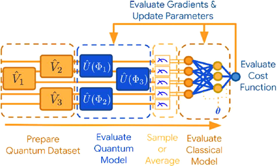 Fig. 5. HQC support vector machine [13].
This algorithm was run on two different IBM quantum computers as well as the qasm simulator as a sort of perfect quantum computer baseline. The accuracy of a classical SVM is 80%, while the accuracy on the simulator is 70%. On the physical devices, the accuracies in both cases are 69%, though it is important to note that accuracies can vary in some cases on different quantum computers [13]. Although the HQC algorithm did not outperform the classical SVM, the relative closeness demonstrates the potential for HQC machine learning to be successful. This work has several future research directions. Instead of binary classification, multiclass classification can be tested with this architecture. The previous discussion on the circle classification highlights that different types of classification are currently better suited to HQC algorithms. The algorithm can also be improved by selecting a better quantum feature map and quantum variational circuit selection. The loss landscape of the QML model can be analyzed to better understand the correlation between data, model training, and accuracy.
Another example is provided by [14]. In this example, a string is represented by bits (either −1 or +1) with a corresponding label (either −1 or +1). A single qubit is used as the readout of the label and the first n qubits are the string representation. Qubits are transformed using some unitary operators (Ui) parameterized on θi. The readout is performed using a Pauli operator, such as σy. The structure of the quantum neural network (QNN) is shown in Fig. 6. In order to reduce the error from the physical devices, the average of observed outcomes is computed. Training is performed in a similar way as the previous example. In this case, each value of θi is randomly generated (though they could also be generated in a structured manner according to the data and the problem). Stochastic gradient descent (GD) is used to learn the parameters [14].
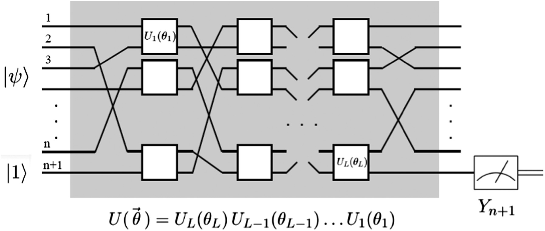 Fig. 6. Quantum neural network [14].
To test this architecture, the authors used the MNIST handwritten digits dataset. The images were reduced to 4 × 4 pixelated images from 16 × 16 to make the algorithm classically simulable on a 17-qubit system. One readout bit is used, so only two numbers can be supported such as 3 and 6. Any ambiguous images that could be either 3 or 6 according to the label are removed. After these changes, 6031 samples remain, down from 5500 for each. A classical attempt is also performed with 16 weights, 1 bias, and 10 internal neurons (170 parameters on internal layer, 4 on output layer). The goal is to match the structure more evenly. Due to reduction to 4 × 4, some samples are identical, meaning that train/test are not completely independent. Less than 1% classification and generalization errors were measured in the classical approach through Matlab [14].
For the quantum architecture, the authors were unsure how to devise the quantum circuit. They did not have good success when using the full set of two-qubit gates. Thus, they reduced the set to only ZX and XX gates. For these two-qubit operations, the first qubit is one of the first 16 and the second is the readout bit. Each full layer of ZX or XX has 16 parameters. Thus, 3 layers of ZX alternating with 3 layers of XX result in 96 parameters. In this test, 2% categorical error was measured. Though this is slightly worse than classical, it shows the potential to learn. This specific example does not make use of exponential (amplitude) storage but can be modified to do so. Without good machine learning practices, the authors achieved a few percent error, so it is feasible to put in superposition [14]. This work has several future research directions. Strategies to reduce the computational cost of putting classical data in superposition can be researched, especially since this encoding needs to be redone every iteration. Better strategies to minimize the loss function than GD could enable faster or more accurate learning. As mentioned earlier, the authors arbitrarily selected some gates since the random approach had poorer accuracy. As such, a more thoughtful selection of gates would likely further increase the accuracy. The initialization of each θi, as mentioned earlier, is another source of potential research.
The two approaches discussed in this section have several key differences. In [13], a support vector machine approach is employed. Each qubit is measured, and support vectors are estimated using a quantum support vector machine simulation. While such an approach has potential for increased accuracy, simulations of quantum systems increase training time and reduce scalability. In contrast, [14] proposes a QNN approach with a single qubit serving as the output layer. This approach can provide only a single classical bit of output, though changes to the architecture could potentially support more. Quantum simulation is not required in this case, providing greater opportunity for scalability. This approach is closer to a NN, whereas the former approach is closer to a hybrid neural support vector machine approach. The advantages and disadvantages in their classical counterparts similarly reflect in these quantum systems. In the next section, the implications of the initial parameterization and methodologies for exploring the loss landscape will be discussed, particularly as they apply to the dangers of reaching a barren plateau.
V.BARREN PLATEAUS
One of the major issues in the use of PQCs for HQC machine learning is barren plateaus. Barren plateaus can occur as a result of parameter initialization or training function. A popular approach is to randomly generate the parameters. However, even if the Haar measure is employed (i.e., the randomness is evenly distributed across the Hilbert space), barren plateaus still occur with high probability in random PQCs. Barren plateaus are positions in the loss function where there is a vanishing gradient, which is an issue that also affects classical deep neural networks (DNNs) [15]. Although the vanishing gradient problem has several solutions in classical DNNs, some of those solutions are not applicable to PQCs. For example, the computing power of classical computers has grown exponentially since the vanishing gradient problem was discovered, allowing a sort of brute force solution. However, NISQ era quantum computers support very few qubits in comparison.
Barren plateaus affect systems with more than a few qubits and systems with more than a few layers. The variance exponentially decays in the number of qubits and quickly converges in the number of layers. This convergence leads to a distinct plateau, with height corresponding to the number of qubits. The variance plateauing causes the gradient to approach 0 (i.e., the vanishing gradient problem) [15]. The future research related to barren plateaus is largely concerned with strategies for overcoming this issue. One such strategy is to perform structured initial guesses. However, the developer may not know enough about the structure of problem. Furthermore, the quantum hardware may not support the structured initial guess. Another strategy is to perform pre-training one segment at a time, akin to one of the solutions to vanishing/exploding gradients in classical DNNs. Another solution to resolving barren plateaus is through a different training methodology. One potential solution is detailed as follows.
The goal of this solution is to explore the loss landscape of the loss function of PQCs. In classical NNs, wider minima basins of the loss function generalize better. These wider basins are achieved in different ways, such as through smaller batches, which is achieved through various hyperparameters. To explore the loss function of PQCs, the Hessian is employed. The Hessian allows detection of local minima, maxima, and saddle points, akin to the second derivative test [16]. One of the issues with implementing the Hessian, therefore, is the calculation of the second derivative of the loss function. Using the limit definition of the derivative to calculate the gradient amplifies the inherent measurement noise. Instead, the authors use parameter shift rules and the chain rule to calculate the Hessian of a quantum circuit [16].
The authors compare GD, quantum natural gradient (QNG), and Hessian optimization methods. The authors propose their own approach, the inverse of the largest eigenvalue of the Hessian. They also compare it to another Hessian-based method, the LBFGS solver, as used in the Pérez-Salinas paper [12,16]. In their testing, the gradients are too small at the beginning, so GD gets stuck. QNG does not seek the steepest direction of the Euclidean space of the parameters but of the distribution space of all possible loss functions. However, QNG can still get stuck in a flat region of the loss function. Thus, QNG has poor performance when the circuit is initialized in a region with small gradients. Although the Hessian methods can help avoid barren plateaus, they struggle with local minima and the Hessian is costlier to calculate than the quantum metric tensor used for QNG [16]. One potential solution to this issue is to use a Hessian approach to escape flat regions of the loss landscape and QNG when the gradient is larger. However, the Hessian may be difficult to properly evaluate on a barren plateau due to measurement noise since the eigenvalues and gradients are small on a barren plateau.
This work has several potential future research directions, such as finding a good approximation scheme for the Hessian of quantum circuits due to the high computational cost. To this end, it may be useful to explore classical approaches to approximating the Hessian vector product in O(n) iterations with n parameters. The learning rate in early SGD determines the quality of the minima found after training, and big initial values, like with the inverse of the Hessian’s largest eigenvalue, may go in this direction. Thus, a combination may be employed. Hessian-based interpretability methods like the influence function may be applied to QNNs. Minimizing PQCs and quantum Monte Carlo can both gain advantages by taking into account the local curvature. Thus, an exploration of their similarities may provide benefits to the training of QNNs. In the next section, we will explore various approaches to improving the accuracy and speed of QML algorithms.
VI.QML IMPROVEMENTS
One of the major problems with HQC machine learning is the finding of optimal parameters for the PQCs. One potential solution is the use of meta-learning, wherein classical NNs are used to rapidly find approximate optima in the parameter landscape for several classes of quantum variational algorithms [17]. In this example, classical recurrent neural networks are used to find optimal parameters for several different algorithms, including Quantum Approximate Optimization Algorithm (QAOA) for MaxCut, QAOA for the Sherrington-Kirkpatrick Ising model, and a Variational Quantum Eigensolver (VQE) for the Hubbard model. The authors claim that this approach learns initial heuristics for both QAOA and VQE that generalize across various problem sizes [17]. A future research direction would be the application of meta-learning in this way to HQC machine learning algorithms that employ PQCs, such as the QNNs discussed in the previous sections.
Another approach to improving QML is the use of ‘hardware-friendly’ circuits that avoid hand-designed modules as much as possible [18]. This example explores HQC NNs with PQCs. There are issues with standard NISQ PQC approaches such as a lack of complete connectivity potentially requiring SWAP gates [8,18]. Furthermore, such implementations rarely beat classical approaches. To overcome these issues, a new approach to QML was proposed. First, a control model is used instead of a gate-based model. In quantum computing, the gate model is one way of representing the evolution of a system using discrete time steps. However, a system can also be modeled using continuous time steps as described by the Schrödinger equation [1]. The time evolution of the Schrödinger equation can be considered as layers of a NN. The number of Arbitrary Waveform Generator periods corresponds to the depth of the NN and the number of qubits corresponds to the width [18]. This approach is technically a generalization of the gate-based approach but more easily adapts to on-chip interconnect topology in more cases than the gate-model approach.
The second major change is in the data encoding methodology. The standard approach encodes the data vector in the quantum state, either as amplitudes or as a binary encoding. The authors propose a data-to-control interface, such as a classical NN, that takes as input the data vector and outputs a set of agent control variables that encode the data in the quantum states [18]. This interface can be a hidden NN layer that feeds into the QNN and can be trained with the rest of the QNN. This approach brings further nonlinearity, an important part of model expressivity [18].
These changes to the structure of the circuit facilitate training, as the problem has been transformed into the optimal control problem. The training steps are GD, sequential perturbation of each hyperparameter, and evaluation of empirical loss via ensemble measurements of the loss function and estimation of its gradient [18]. This approach was tested on the MNIST handwritten digits dataset. The test employed three qubits and classified between eight digits, as three bits can distinguish at most eight digits. The authors achieved lower than 10% error. They claim this is only possible with PQC approaches with a downsized dataset (e.g., binary classification or downsized images) or with more qubits (i.e., nine or more) [18]. The related future research areas include exploring this approach’s potential on more complicated learning tasks and exploring the application of the novel data encoding approach in PQC gate-based methods. The next section will discuss the application of these QML techniques to QCNNs.
VII.QUANTUM CONVOLUTIONAL NEURAL NETWORK
QCNNs provide support for solving quantum many-body problems, such as quantum phase recognition and QEC optimization [19]. As such, QCNNs are of particular interest in the NISQ era, where error correction is vital in certain applications. A classical convolutional neural network (CNN) is composed of three types of layers, the convolution layer, the pooling layer, and the fully connected layer. In one example, the authors use a single quasilocal unitary that is applied in a translationally invariant manner as the convolution layer. The pooling layer is implemented by measuring some of the qubits and using those results to determine which unitary rotations should be applied to nearby qubits, thereby reducing the degrees of freedom and introducing nonlinearity. The fully connected layer is a unitary gate. In their experiments, the authors found this approach better at QEC than Shor code and no error correction [19].
The following is another potential approach to implementing a QCNN, including convolution layers, pooling layers, and fully connected layers. For the convolution layer, filters are typically non-reversible and the expense of calculating the gates multiple times to support ancilla qubits grows exponentially. Thus, the authors present a novel approach using a linear combination of unitary operations that takes advantage of an extra first and last column of data. These extra columns can be used without affecting the image detection results [20]. The pooling layer is implemented as average pooling. The authors claim that by ignoring certain qubits, the pooled output can be directly realized [20]. The fully connected layer is implemented using a parameterized Hamiltonian composed of identity operators and Pauli-Z operators. The parameters can be learned using GD and classical backpropagation [20].
To test this architecture, the authors use the MNIST handwritten number dataset. The authors manually simulate noise to simulate the behavior of a physical NISQ era quantum computer. They look at two problems, two-digit classification (1 and 8) and any-digit classification (0–9). In their approach, there are significantly fewer learnable parameters, with 46 for two-digit and 379 for any-digit, compared to a classical CNN with 265 and 2569 parameters, respectively. The noise-free QCNN accuracy versus the CNN accuracy of the test dataset is 74.3% versus 80.4% for any-digit classification and 96.3% versus 97.2% for two-digit classification. The future related research could include demonstrating the accuracy of this approach on physical NISQ era quantum computers, exploring other alternatives for the three types of layers, applying different learning methods, and exploring the accuracy on different types of image datasets.
VIII.CONCLUSIONS
In this paper, we provided a brief introduction to NISQ era, gate-model quantum computing. These platforms can be employed for various machine learning tasks. We discussed several major applications of PQCs in HQC algorithms for machine learning. There are many potential research directions related to this topic, as discussed throughout this paper. These directions include avoiding barren plateaus, selection of better PQCs, exploring different learning algorithms, and applying QML to various datasets using physical quantum computers. A major future milestone would include the creation of QML algorithms that outperform their classical counterparts.