I.INTRODUCTION
Steel surfaces have broad uses in various industries such as automobiles, marine, electronics, etc. Ensuring the quality of industrial production, especially for steel surfaces, is highly dependent on conducting defect inspections as an essential step. Various environmental conditions encountered during steel surface production can lead to the generation of defects. These defects are apparent in diverse forms, such as Roll marks, attributed to irregular roller shapes or excessive curling, scales primarily resulting from greasy residue on work rollers during temper rolling and incomplete removal of impurities, and Scratches, which arise from friction between the rolled product and equipment components like worn or damaged guides [1]. These defects significantly compromise the quality of steel strips and can result in customer rejection, causing financial losses for the production plant [2]. Effective defect detection and classification are imperative for quality control in steel surface inspection. Defect detection seeks to identify the presence and location of defects in surface images, facilitating early inspection to minimize losses. Meanwhile, defect classification aims to categorize defects into specific categories, aiding in the identification and understanding of different defect types [3]. Surface defect inspection methods based on deep learning have been proven to be more stable than traditional machine learning and statistical methods. As a result, many researchers have shifted towards using deep learning methods for surface defect inspection. Due to the high resource requirements for training deep learning models on large datasets, transfer learning approaches are commonly used. Due to the constant progress in developing CNNs for identifying steel surface defects, relying on individual models like MobileNet [4] and visual geometry group (VGG) [5] is no longer sufficient to meet current demands. This is because each model has its own work bias. Hence, the ensemble approach can combine the strengths of different models, resulting in a more optimal classification of steel surface defects. Furthermore, this study combines outputs of three different transfer learning models through ensemble learning that help achieve a better accuracy rate. The primary contributions of this paper are as follows:
- 1.Provide a more accurate and stable deep learning-based steel surface defect classification prediction mode.
- 2.Comparing the ensemble-method-based model with base models using recognized assessment measures to prove its superiority.
- 3.Leveraging the strengths of base models to mitigate their weaknesses through combined predictions.
- 4.Comparative analysis is conducted to demonstrate the effectiveness of the proposed ensemble method in comparison to other studies.
The remainder of this paper is structured as follows: Section II discusses related work. Section III presents details of the base models and the proposed ensemble approach. Section IV encompasses the experimental results and visual analysis. Section V compares the proposed model with existing methods. Finally, Section VI concludes the paper.
II.BACKGROUND AND RELATED WORKS
A.TRANSFER LEARNING
Transfer learning involves using knowledge acquired from previous tasks to improve performance on a new, related task. In the context of deep learning, it allows models pre-trained on large-scale datasets to be adapted for specific applications, reducing computational costs and improving generalization. By leveraging this concept, defect image datasets can be effectively classified by adapting pre-trained models from ImageNet Zou et al. [27]. Unlike traditional feature-based methods such as SIFT, BRISK, and HOG, transfer learning methods include low- to high-level features, thereby providing richer semantic information and improved representation of defective images. Employing transfer learning methods has shown that they can substantially decrease the time needed to train deep learning models [6]. It enhances performance and is faster than building a model from the beginning [30]. For transfer learning to be effective, there must be a correlation between the features learned from the source domain (ImageNet) and the target domain (steel surface defect classification). Although ImageNet primarily consists of natural images, its pre-trained CNN models capture fundamental image properties, such as edges, textures, and object structures, which are highly relevant to defect detection. Steel surface defects often exhibit distinctive texture variations, patterns, and structural inconsistencies, which can be effectively detected using the hierarchical feature representations learned by CNNs. The lower layers of pre-trained models detect basic edges and textures, while the deeper layers capture more complex patterns—both of which are crucial for distinguishing between different defect types. Moreover, transfer learning significantly mitigates the challenge of limited training data. Training a deep CNN from scratch requires a large, labeled dataset to generalize well, but steel defect datasets such as NEU and X-steel surface defect (X-SDD) have relatively small sample sizes. By fine-tuning pre-trained models, the knowledge acquired from large-scale datasets can be transferred to the defect classification task, improving accuracy while reducing the risk of overfitting. Prior research supports the effectiveness of this approach [9–11,21]; for instance, Fu et al. [7] demonstrated that adapting pre-trained SqueezeNet models significantly enhances classification performance, while Abu et al. [6] found that MobileNet, ResNet, and VGG-based models perform well in defect identification. These findings indicate that transfer learning provides a robust and efficient steel surface defect classification method. Research indicates that employing Transfer Learning with pre-trained models is a valuable strategy to enhance performance when dataset sizes are limited. This study introduces an ensemble method that leverages various pre-trained Convolutional Neural Network models, aiming to capitalize on the strengths of each model. The rationale is that a defect misclassified by one base model might be correctly identified by another. Consequently, integrating multiple pre-trained CNN models can notably improve recognition rates compared to relying solely on individual models.
B.ENSEMBLE LEARNING
Ensemble learning is a strategy that integrates multiple models or diverse predictions to enhance performance across various tasks, including classification, prediction, and function approximation [12,13,26]. Recent scholarly efforts have explored ensemble learning for classifying the defects that appear on steel surfaces. Chen et al. [14] introduced an ensemble approach for steel surface defect recognition, where three distinct DCNN models underwent individual training. Subsequently, an averaging strategy was employed to combine their outputs, resulting in a recognition rate of 99.889% using the NEU dataset. Akhyar et al. [15] proposed an ensemble method that integrates super-resolution techniques, boundary localization, and sequential feature pyramid networks to enhance steel surface inspection. Konovalenko et al. [16] evaluated the application of RNN in recognizing industrial steel defects. In contrast, Bouguettaya et al. [28] introduced a technique combining two pre-trained models, MobileNet-V2 and Xception, to categorize six types of surface defects appearing on hot-rolled steel strips. Liu et al. [29] addressed the problem of poor accuracy and low processing in conventional approaches for detecting defects on steel surfaces by utilizing Extreme Learning Machines. In summary, significant efforts have been dedicated to developing inspection systems for automatically detecting and classifying defects on steel surfaces. Research indicates that employing Transfer Learning with pre-trained models is a valuable strategy to enhance performance when dataset sizes are limited. This study introduces an ensemble method that leverages various pre-trained convolutional neural network models, aiming to capitalize on the strengths of each model. The rationale is that a defect misclassified by one base model might be correctly identified by another. Consequently, integrating multiple pre-trained CNN models can notably improve recognition rates compared to relying solely on individual models.
III.MATERIALS AND METHODS
This section provides details of the base models and the proposed ensemble model.
A.TRANSFER LEARNING USING INCEPTION-V3, VGG16, AND MOBILENET-V2 NETWORKS
Inception-v3 is a pre-trained CNN that is 48 layers deep developed by Szegedy et al. [27] to address issues related to computational efficiency and low parameters in practical applications. This network version has undergone training on over a million images from the ImageNet dataset. As a result, there are extensive feature representations for various types of images. In terms of specifications, it accepts input images of size 299 × 299 and functions in two stages: initially, it extracts general features from the input images, and subsequently, it utilizes these features to classify the images.
VGG16 is a CNN model trained for image classification tasks developed by Simonyan [18]. It is an improved version of AlexNet. VGG 16 has 16 convolutional and fully connected layers with an input image size of 224×224×3. It has a simple and uniform architecture, with all convolutional layers having a kernel size of 3×3 and a stride of 1 and all pooling layers having a kernel size of 2×2 and a stride of 2.
MobileNet is a computer vision model proposed by Howard [4] that offers a solution to the challenge of a sharp increase in the number of parameters that often accompany deeper neural network architectures in computer vision. It achieves this by leveraging depth-wise convolutions, which transform standard convolutions into depth-wise separable convolutions, thereby substantially diminishing parameter counts compared to alternative networks—resulting in a lightweight deep neural network.
B.PROPOSED ENSEMBLE LEARNING MODEL
In our study, we have chosen three transfer learning models, including Inception V3, VGG16, and MobileNet, to build an ensemble model. Their distinct characteristics and capacity guided the choice of these models to meet the need for diversity in ensemble learning, where ensuring high diversity and predictive performance is crucial when selecting the participating base models. This paper combines the above pre-trained model architectures to capture their strengths, leveraging their prior training on extensive datasets such as ImageNet. This approach enables the learning of features specific to the target task, such as classifying defects on steel surfaces, even when confronted with a limited dataset. In other words, the discriminative features learned by these pre-trained architectures on ImageNet can seamlessly transfer to our dataset, enhancing performance and adaptability. Figure 1 clearly shows the proposed ensemble method’s flow chart for the classification of steel surface defects.
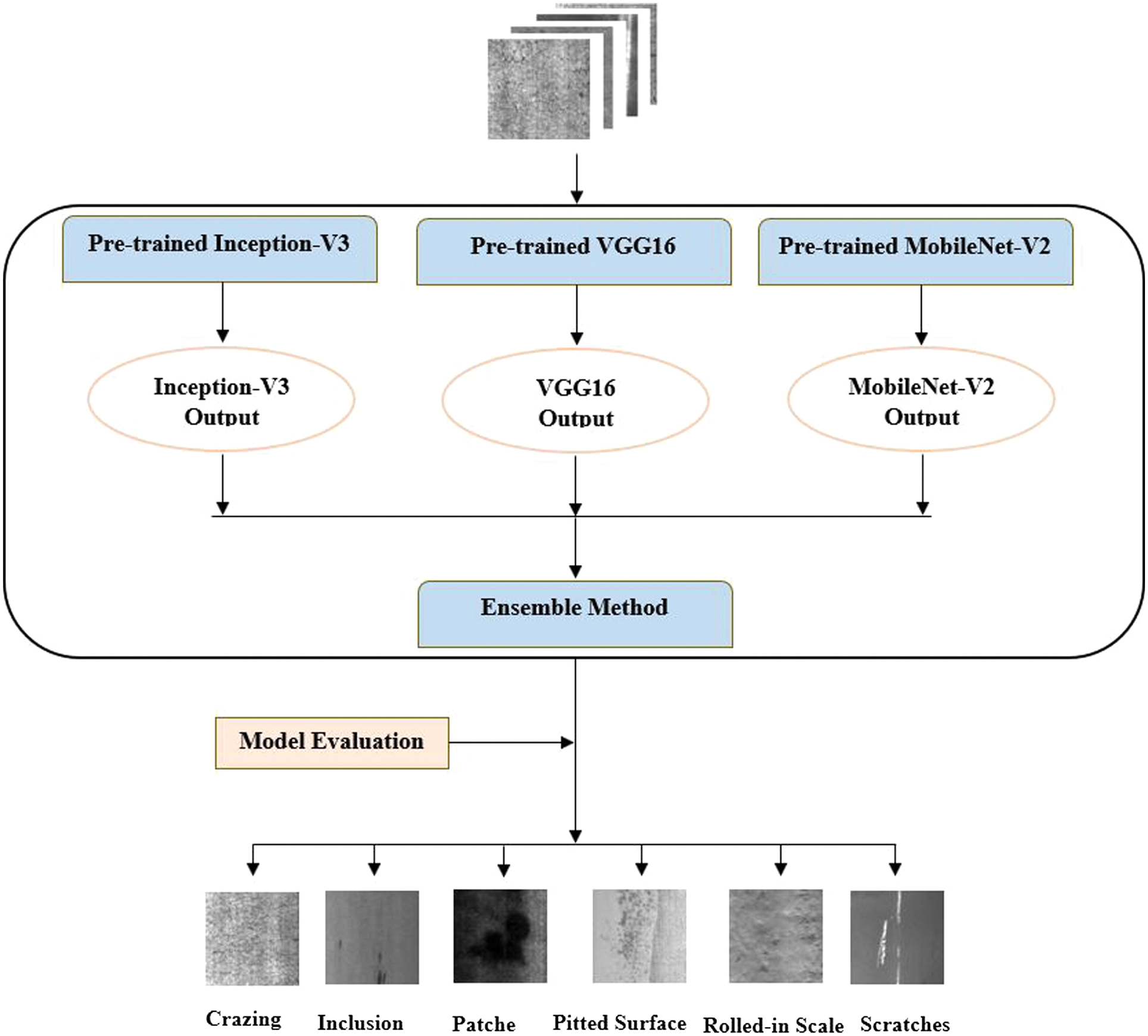 Fig. 1. Flow chart of the proposed ensemble model for steel surface defect classification.
As the depth of a deep CNN model increases, the parameter count rises, aiming to improve efficiency. Consequently, large datasets are required for training, significantly increasing computational demands. Directly applying the pre-trained models to small datasets leads to inducing bias in feature extraction, overfitting, and restricted generalization capabilities. Consequently, we modified the three pre-trained models and adjusted their architectures to suit the characteristics of the two datasets that we are using. Hyperparameters were configured for the three pre-trained models considered base models and the proposed ensemble method applying on NEU and X-SDD datasets, as outlined in Table I.
Table I. The parameter settings of the base models and the proposed ensemble model applied on NEU and X-SDD datasets
| Dataset | Approach | Initial input size | Learning rate | Optimizer | Batch size | Epochs |
|---|---|---|---|---|---|---|
| NEU | Inception-V3 | 224 × 224 | 1e-4 | Adam | 42 | 50 |
| VGG16 | 224 × 224 | 1e-4 | Adam | 42 | 50 | |
| MobileNet | 224 × 224 | 1e-4 | Adam | 42 | 50 | |
| Ensemble model | 224 × 224 | 1e-4 | Adam | 32 | 50 | |
| X-SDD | Inception-V3 | 224 × 224 | 1e-4 | Adam | 20 | 50 |
| VGG16 | 224 × 224 | 1e-4 | Adam | 16 | 50 | |
| MobileNet | 224 × 224 | 1e-4 | Adam | 20 | 50 | |
| Ensemble model | 224 × 224 | 1e-4 | Adam | 20 | 50 |
The three base models are trained individually, and the best-trained model is selected based on the accuracy rate achieved on the testing set. The proposed ensemble prediction method is modeled as follows:
Training:
Prediction:
Ensemble:
Equation (1) represents the process of training using a training dataset Dtrain and validating it using a validation dataset Dval where the Mk refers to the base models. The training involves optimizing the model’s parameters using the Adam optimizer over a specified number of epochs. Equation (2) denotes the prediction process for a given trained model . Here, Dtest represents the testing set, and the function predict(·) is applied to perform the test on a dataset using the trained model . The outputs yi and pi correspond to the predicted value and its probability for the test dataset. Equation (3) represents the proposed ensemble method that gives the ultimate prediction. For each model of base models, the training set is used to calculate the probability. The ensemble model’s final output is generated by summing the products of predictions from the base models, each multiplied by its respective probability, using the training data. The pseudo-code of this process is provided by Algorithm 1.
Algorithm 1: Proposed Ensemble Learning Algorithm with Inception V3, VGG16, and MobileNet
| |
| |
| 1 |
| 2 Initialize all layers for Mk; |
| 3 Generate using Equation |
| 4 |
| 5 |
| 6 Generate (yipi) using Equation |
| 7 |
| 8 Generate P using Equation |
This approach leverages the diversity of base models to enhance the overall predictive performance. It enables the correction of errors from individual models by leveraging the strengths of others, resulting in an ensemble output that surpasses any single participating model.
IV.EXPERIMENTAL RESULTS & DISCUSSION
A.EXPERIMENTAL ENVIRONMENT AND DATASETS
To assess the effectiveness of our proposed method in classifying hot-rolled steel defects, we utilize two widely recognized benchmark datasets: the X-SDD dataset and the Northeastern University Surface Defect (NEU) dataset. Our testing environment comprises an Nvidia GeForce 940MX graphics card, an Intel Core i5-7200 CPU operating at 2.60 GHz, 16GB of RAM, and runs on the Windows 10 operating system. We implement the Keras deep learning framework to conduct our experiments. In this study, we employ the popular evaluation metrics, including accuracy, precision, recall, and F1-score, as performance metrics to assess the base methods and the proposed ensemble model. These metrics are calculated using the following equations:
The confusion matrix, as depicted in Table II, illustrates the various outcomes of our method. A true positive (TP) denotes the number of positive samples correctly classified, while a true negative (TN) indicates a negative sample correctly identified as negative. Conversely, a false positive (FP) occurs when a negative sample is erroneously identified as positive, and a false negative (FN) transpires when a positive sample is incorrectly labeled as negative.
Table II. The various outcomes of the proposed method
| Predicted Class | |||
|---|---|---|---|
| Positives | Negatives | ||
| True Class | Positives | TP | FN |
| Negatives | FP | TN | |
B.RESULTS ON NORTHEASTERN UNIVERSITY SURFACE DEFECT DATASET
The northeastern dataset was compiled by Song Kechen’s team at Northeast University of China [8], which is a widely recognized benchmark for assessing the performance of steel surface defect classification models. It consists of 1800 grayscale images, each with a 200×200 pixels resolution. This dataset encompasses six distinct types of typical defects found on the surface of hot-rolled steel strips, with 300 samples allocated to each defect type. These defect types include inclusion (In), patches (Pa), crazing (Cr), pitted surface (PS), rolled-in scale (RS), and scratches (Sc). Sample images showcasing some of these typical defects are illustrated in Fig. 2.
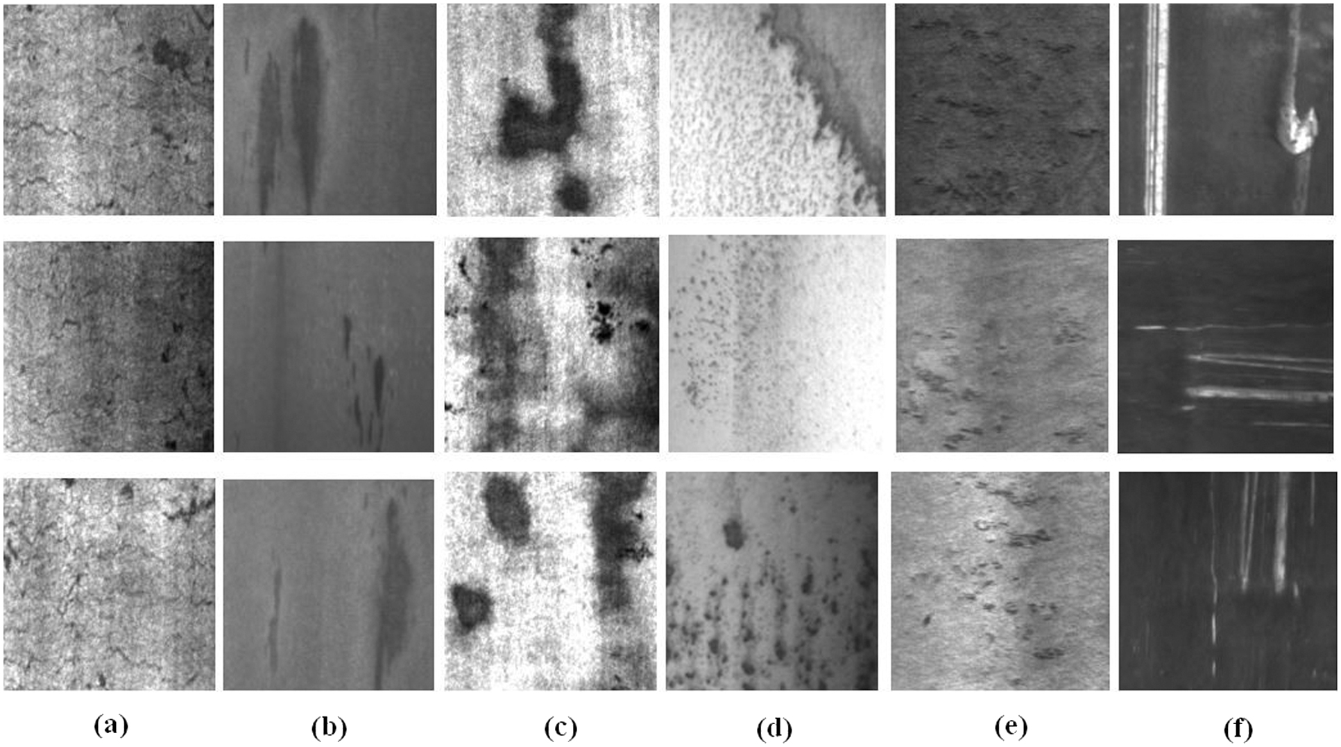 Fig. 2. Samples for the six kinds of defect classes of the NEU dataset including (a) crazing (Cr), (b) inclusion (In), (c) patches (Pa), (d) pitted surface (Ps), (e) rolled-in scale (Rs), (f) scratches (Sc).
In terms of training of base models and the proposed ensemble model, the dataset was split into three subsets in the experimental setup: a training set with 864 images, a test set with 360 images, and the rest of the images assigned to the validation set. Subsequently, both the base models and the suggested ensemble model were assessed on the test set to determine their classification accuracy. Table III presents the classification accuracy obtained by the base models and the proposed ensemble model using the NEU dataset. As shown in Table III, the proposed ensemble approach effectively classifies hot strip defects.
Table III. Classification results of base models and ensemble model using NEU dataset
| Model | Accuracy |
|---|---|
| VGG16 | 98.88% |
| Inception-V3 | 99.16% |
| MobileNet | 99.16% |
| Proposed ensemble model |
C.RESULTS ON X-DD SURFACE DEFECT DATASET
The X-SDD surface defect dataset, publicly available for hot-rolled steel surface defects, comprises 1360 images with 128×128 pixels resolutions. This dataset is organized into seven distinct categories of surface defects, including 63 oxide scale of plate system, 397 red iron sheets, 238 inclusions, 134 surface scratches, 122 iron sheet ash, 203 finishing roll printing, and 203 oxide scale of temperature system Feng et al. [17]. Figure 3 shows sample images representing these seven typical surface defects.
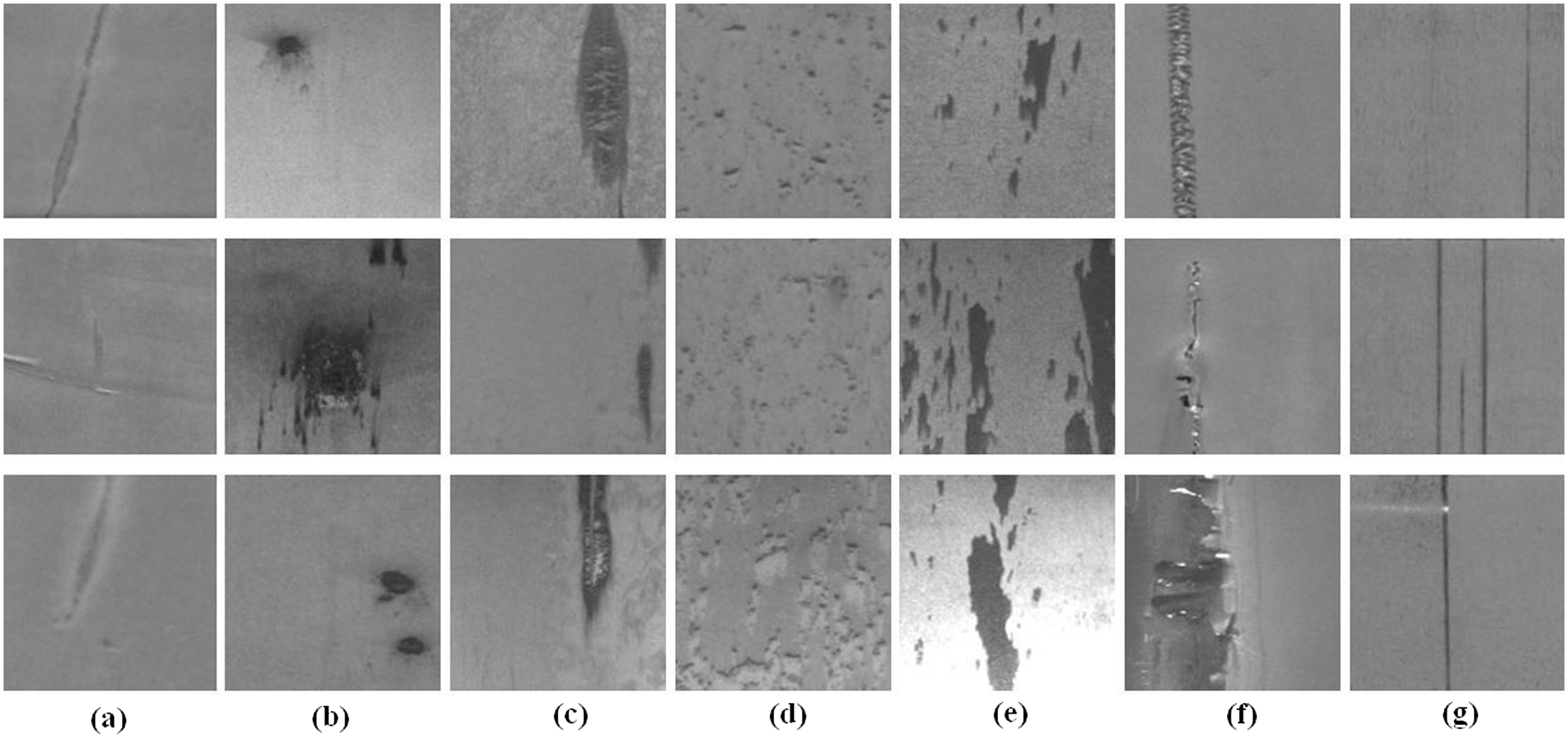 Fig. 3. Samples for the seven kinds of defect classes of the X-SSD dataset including (a) finishing roll printing (Fr), (b) iron sheet ash (Is), (c) oxide scale-of-plate system (Op), (d) oxide scale-of-temperature system (Ot), (e) red iron sheet (Ri), (f) inclusion (Si), (g) scratches (Ss).
Our next experiment split the X-SDD dataset into three subsets: a training set with 739 images, a test set with 137 images, and the rest of the images assigned to the validation set. Dropout regularization was implemented in the fully connected layers with a dropout rate of 0.5. Table IV presents the classification results achieved by the base models and the proposed ensemble model using the X-SDD dataset. These results provide insights into the efficacy of our approach in accurately classifying surface defects within the hot-rolled steel dataset. The classification reports, as summarized in Table V, show variations in the performance of different base models across the NEU and X-SDD datasets. Upon comparison of the results in Table V, it becomes clear that the proposed ensemble model applying to the NEU dataset surpasses all individual participating models across all three metrics, in which it achieves a classification accuracy of 100% across all indicators, signifying the balanced performance of our method across all metrics.
Table IV. Classification results of base models and ensemble model using the X-SDD dataset
| Model | Accuracy |
|---|---|
| VGG16 | 95.62% |
| Inception-V3 | 97.81% |
| MobileNet | 91.24% |
| Proposed ensemble model |
Table V. Results of three base models and the proposed ensemble model. The first row’s fourth to sixth columns denote three evaluation matrices. The second to the last rows in the first column denote transfer learning and the proposed ensemble model, respectively. The second to the last rows in the second column denote two datasets used. The second to the last rows in the third column denote the type of defects of each dataset
| Approach | Dataset | Type of defect | Precision | Recall | F1 score | Support |
|---|---|---|---|---|---|---|
| Cr | 100% | 100% | 100% | 60 | ||
| Inception-V3 | In | 100% | 0.95% | 0.97% | 60 | |
| NEU | Pa | 100% | 100% | 100% | 60 | |
| Ps | 0.95% | 100% | 0.98% | 60 | ||
| Rs | 100% | 100% | 100% | 60 | ||
| Sc | 100% | 100% | 100% | 60 | ||
| FRP | 100% | 100% | 100% | 21 | ||
| ISA | 100% | 0.92% | 0.96% | 12 | ||
| OSPS | 100% | 100% | 100% | 6 | ||
| X-SDD | OSTS | 0.95% | 100% | 0.98% | 20 | |
| RI | 100% | 100% | 100% | 40 | ||
| SI | 100% | 100% | 100% | 24 | ||
| SC | 100% | 100% | 100% | 14 | ||
| VGG16 | Cr | 100% | 100% | 100% | 60 | |
| In | 0.98% | 0.98% | 0.98% | 60 | ||
| NEU | Pa | 0.98% | 0.98% | 0.98% | 60 | |
| Ps | 0.98% | 0.97% | 0.97% | 60 | ||
| Rs | 100% | 100% | 100% | 60 | ||
| Sc | 0.98% | 100% | 0.99% | 60 | ||
| FRP | 100% | 0.95% | 0.98% | 21 | ||
| ISA | 0.92% | 100% | 0.96% | 12 | ||
| OSPS | 100% | 0.67% | 0.80% | 6 | ||
| X-SDD | OSTS | 0.95% | 100% | 0.98% | 20 | |
| RI | 0.95% | 100% | 0.98% | 40 | ||
| SI | 0.96% | 0.92% | 0.94% | 24 | ||
| SC | 0.93% | 0.93% | 0.93% | 14 | ||
| Cr | 100% | 100% | 100% | 60 | ||
| MobileNet | In | 0.97% | 0.98% | 0.98% | 60 | |
| NEU | Pa | 100% | 100% | 100% | 60 | |
| Ps | 100% | 0.97% | 0.98% | 60 | ||
| Rs | 100% | 100% | 100% | 60 | ||
| Sc | 0.98% | 100% | 0.99% | 60 | ||
| FRP | 100% | 0.86% | 0.92% | 21 | ||
| ISA | 0.65% | 0.92% | 0.76% | 12 | ||
| OSPS | 0.83% | 0.83% | 0.83% | 6 | ||
| X-SDD | OSTS | 100% | 0.90% | 0.95% | 20 | |
| RI | 0.95% | 0.95% | 0.95% | 40 | ||
| SI | 0.92% | 0.96% | 0.94% | 24 | ||
| SC | 0.92% | 0.86% | 0.89% | 14 | ||
| Ensemble model | Cr | 100% | 100% | 100% | 60 | |
| In | 100% | 100% | 100% | 60 | ||
| NEU | Pa | 100% | 100% | 100% | 60 | |
| Ps | 100% | 100% | 100% | 60 | ||
| Rs | 100% | 100% | 100% | 60 | ||
| Sc | 100% | 100% | 100% | 60 | ||
| FRP | 100% | 0.95% | 0.98% | 21 | ||
| ISA | 0.92% | 100% | 0.96% | 12 | ||
| OSPS | 100% | 100% | 100% | 6 | ||
| X-SDD | OSTS | 100% | 100% | 100% | 20 | |
| RI | 100% | 100% | 100% | 40 | ||
| SI | 100% | 100% | 100% | 24 | ||
| SC | 100% | 100% | 100% | 14 |
D.VISUALIZED ANALYSIS
In order to visually evaluate the classification performance of both the base models and our proposed ensemble model, we present confusion matrices and fractions of wrong predictions for each individual model. These visualizations provide a more intuitive understanding of the classification accuracy of our proposed method across different defect categories. Figures 4 and 5 display the confusion matrices and fractions of incorrect predictions, respectively, for the base models applied to the NEU and X-SDD datasets. The numbers in Fig. 4 indicate the count of images correctly or incorrectly predicted per class. In contrast, Fig. 5 quantifies the prediction errors as a fraction of total samples in each class, helping visualize model-specific weaknesses. On the other hand, Figs. 6 and 7 present the confusion matrices and fractions of incorrect predictions for the proposed ensemble model on the NEU and X-SDD datasets.
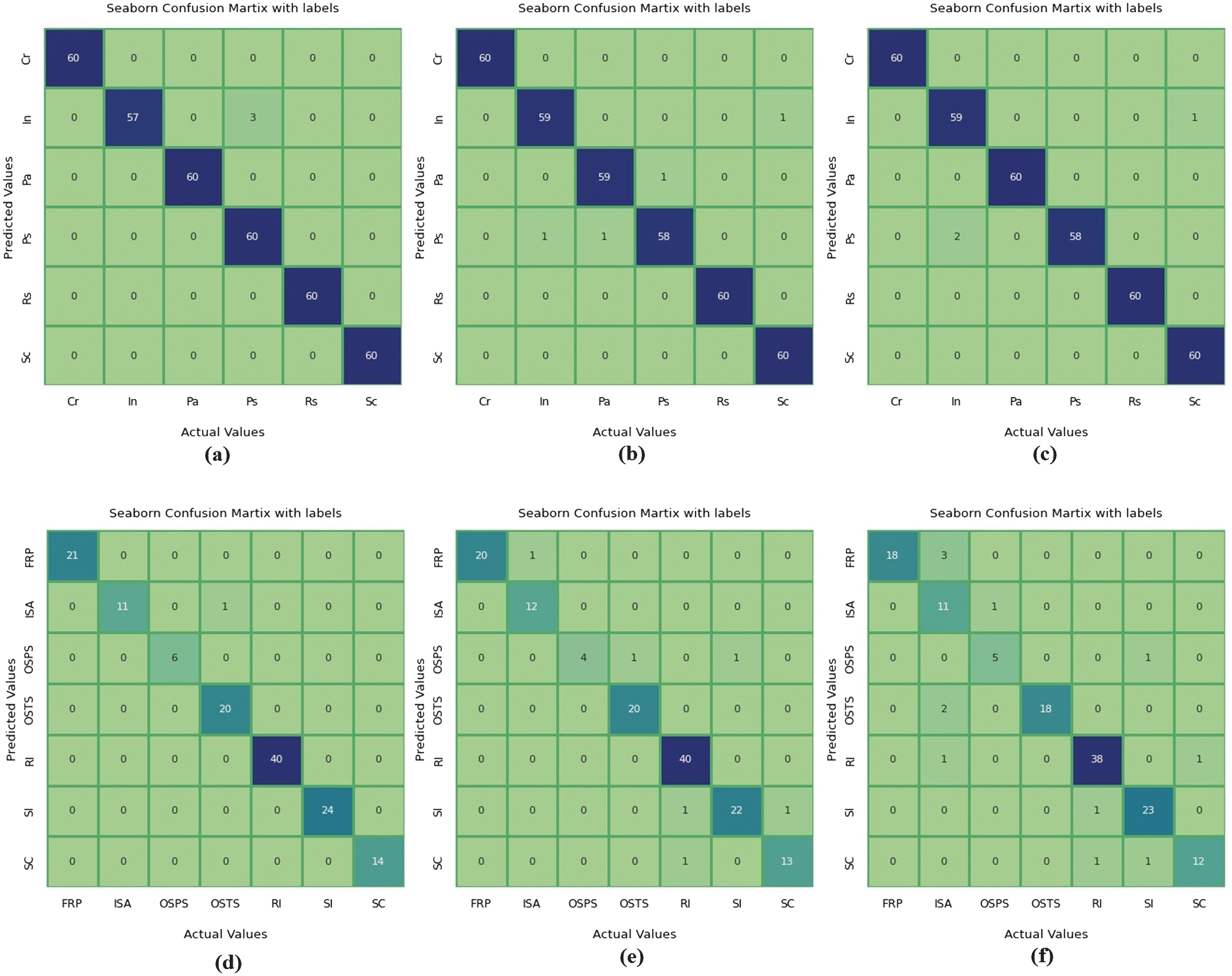 Fig. 4. (Top) Confusion matrix of base models for classification of the six types of hot-rolled steel surface defects on the NEU dataset: (a) Inseption-V3, (b) VGG16, (C) MobilNet. (Down) Confusion matrix of base models for classification of the seven types of hot-rolled steel surface defects on the X-SDD dataset: (d) Inseption-V3, (e) VGG16, (f) MobilNet.
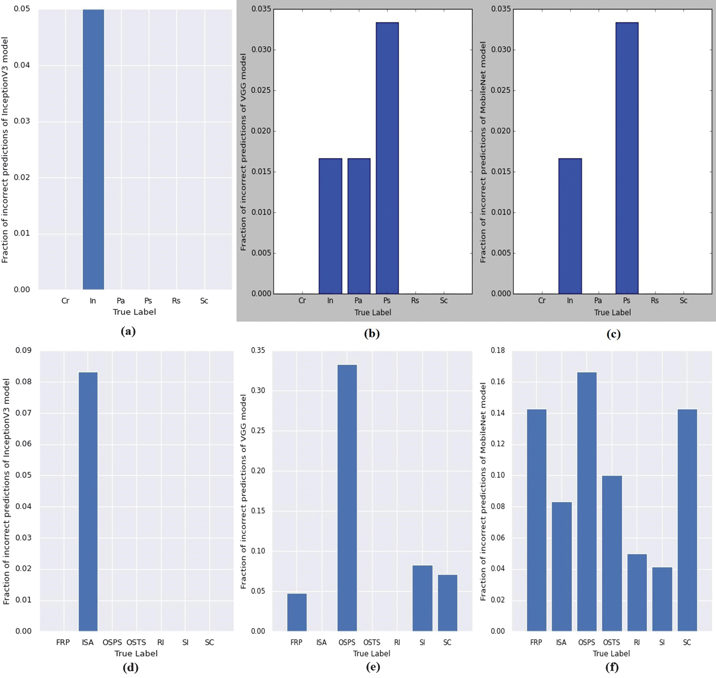 Fig. 5. (Top) Fraction of incorrect predictions of the base models for classification of the six types of hot-rolled steel surface defects on the NEU dataset: (a) Inseption-V3, (b) VGG16, (C) MobilNet. (Down) Fraction of incorrect predictions for seven types of hot-rolled steel surface defects on the X-SDD dataset: (d) Inseption-V3, (e) VGG16, (f) MobilNet.
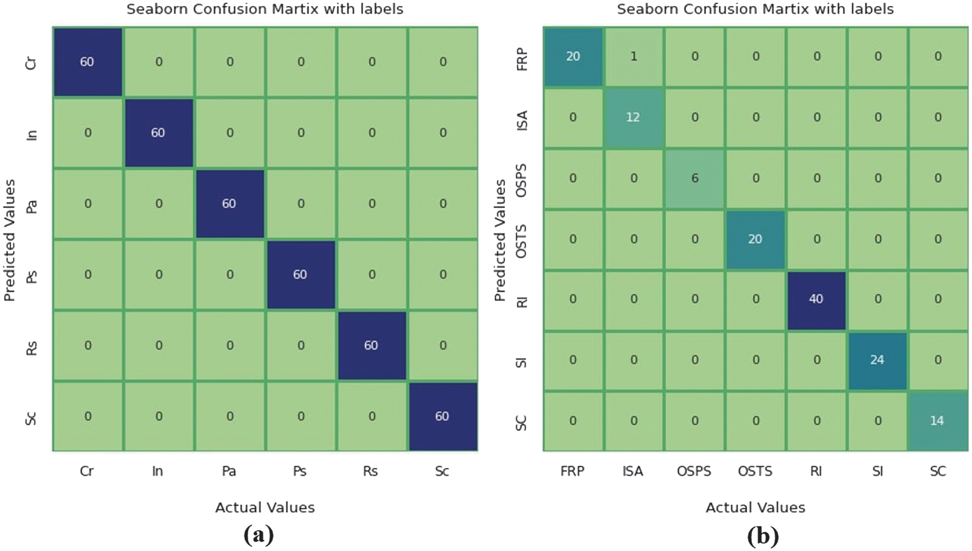 Fig. 6. (a) Confusion matrix of the proposed ensemble model for classification of the six types of hot-rolled steel surface defects on the NEU dataset. (b) Confusion matrix of the proposed ensemble model for classification of the seven types of hot-rolled steel surface defects on the X-SDD dataset.
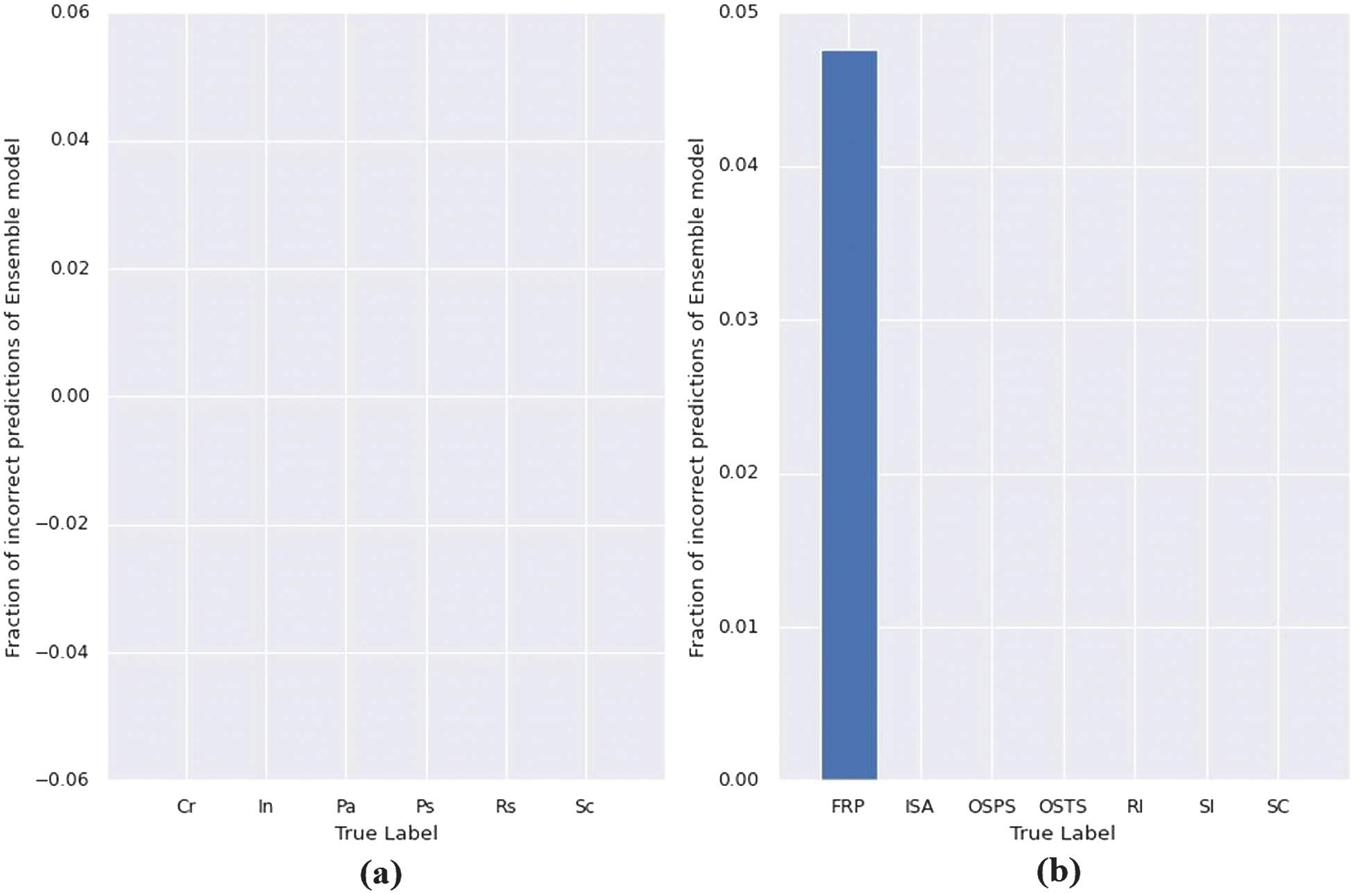 Fig. 7. (a) Fraction of incorrect predictions of the proposed ensemble model for classification of the six types of hot-rolled steel surface defects on the NEU dataset. (b) Fraction of incorrect predictions of the proposed ensemble model for classification of the seven types of hot-rolled steel surface defects on the X-SDD dataset.
We can observe from Fig. 6 that our proposed ensemble method achieves exceptional classification accuracy for every category in the NEU dataset.
It achieves a perfect 100% accuracy for each class, with no incorrect predictions across any of the classes which is illustrated in Fig. 7(a). However, in the X-SDD dataset, as illustrated in the confusion matrix of Fig. 7, our method demonstrates accurate classification for most defect types, with slightly lower accuracy observed for the finishing roll printing category. Specifically, our model achieves 20 correct classifications and one incorrect classification for finishing roll printing. This decrease in accuracy may be attributed to the insufficient data available for this particular defect type, hampering the effective learning process of our model.
V.COMPARISONS WITH STATE-OF-THE-ART
We conducted a comparative analysis to assess the accuracy achieved by our proposed ensemble model against existing methods reported in [20,22,24,25], which were implemented on the NEU dataset. Table VI summarizes the comparison results. DenseNet, a transfer learning method based on CNN, demonstrates the significant impact of network depth, feature extraction network, and feature transformation methods on sample classification accuracy. Additionally, BYEC, employing an evolutionary Bayesian classifier, exhibits comparatively inadequate precision rates. ADRS, utilizing traditional CNN, is affected to some extent by the small database size, influencing classification results. AECLBP, using enhanced LBP features, shows improved classification compared to traditional LBP features but lags significantly behind CNN-based feature extraction. Similarly, we compared the accuracy attained by our proposed ensemble model with existing methods reported in [17,19], implemented on the X-SDD dataset. As depicted in Table VI, our proposed ensemble model achieves a classification accuracy of 99.27%, outperforming the accuracies reported in [23] (94.85%), [17] (95.10%), and [19] (99.00%).
Table VI. Comparison of classification accuracy of different methods applied on NEU and X-SDD datasets
| Dataset | Model | Accuracy |
|---|---|---|
| DenseNet [ | 92.33% | |
| NEU | BYEC [ | 96.30% |
| ADRS [ | 98.10% | |
| AECLBP [ | 98.87% | |
| Ensemble model [ | 99.889% | |
| Proposed ensemble model | ||
| Ensemble model [ | 94.85% | |
| X-SDD | RepVGG B3g4+SA [ | 95.10% |
| Zero-shot [ | 99.00% | |
| Proposed ensemble model |
Table VII presents a comparative analysis of classification accuracy achieved by various ensemble methods on the NEU and X-SDD datasets. Our proposed ensemble model consistently outperformed existing methods. On the NEU dataset, while Vasan et al. [31] and Bouguettaya et al. [32] achieved 99.72% accuracy and Chen et al. [14] reached 99.89% through deep CNN ensemble techniques, our model attained a perfect 100%, demonstrating its robustness in integrating multiple pre-trained CNN architectures to minimize misclassification. Similarly, for the X-SDD dataset, where Feng et al. [23] reported 94.85% accuracy and Hussain et al. [33] improved it to 98.89%, our ensemble model further enhanced classification accuracy to 99.27%, showcasing its effectiveness in handling diverse defect types. The model’s strength lies in integrating Inception-V3, VGG16, and MobileNet, ensuring a well-balanced feature extraction process that reduces bias and variance. The remarkable 100% classification accuracy on the NEU dataset is attributed to multiple factors, including the dataset’s well-defined defect categories with distinct visual features, making classification less ambiguous. Integrating Inception-V3, VGG16, and MobileNet, our ensemble approach enhances feature extraction and mitigates weaknesses in individual models, significantly reducing misclassification errors. The dataset’s structure, with a limited number of defect classes and sufficient sample representation, further minimized class imbalance and feature overlap, ensuring high predictive reliability. While machine learning models generally exhibit some uncertainty, combining optimized hyperparameters, transfer learning, and an ensemble decision mechanism contributed to superior accuracy. However, real-world applications may introduce additional complexities, such as varying lighting conditions and surface textures, which could impact classification performance. Future research should focus on testing the model on more complex datasets to validate its adaptability and robustness further.
Table VII. Comparison of classification accuracy of ensemble methods applied on NEU and X-SDD datasets
| Dataset | Reference | Accuracy |
|---|---|---|
| Vasan et al. [ | 99.72% | |
| NEU | Bouguettaya et al. [ | 99.72% |
| Chen et al. [ | 99.89% | |
| Feng et al. [ | 94.85% | |
| X-SDD | Hussain et al. [ | 98.89% |
Ensemble methods inherently introduce additional computational overhead compared to single-model approaches due to multiple model evaluations and aggregation processes. The time complexity of the proposed ensemble model can be analyzed by considering the base models: Inception-V3, VGG16, and MobileNet. Each model has a computational complexity of O(nm2), where n represents the number of layers, and m denotes the feature map size. Since the ensemble model integrates these architectures, the total complexity is approximately O(k×nm2), where k is the number of models used in the ensemble. This increases inference time compared to single models, which individually have a complexity of O(nm2). Although ensemble learning increases processing time, its advantages in accuracy and robustness justify its use, particularly in industrial applications where defect classification precision is critical.
VI.CONCLUSION
We introduced an ensemble model for the classification of steel surface defects, leveraging three transfer learning models: VGG16, MobileNet, and Inception-V3. The proposed ensemble model exhibited exceptional classification accuracy, surpassing 99% on the X-SDD dataset and achieving a perfect 100% on the NEU dataset, outperforming several existing methods. This underscored its practical efficacy in accuracy in steel strip defect classification. However, despite the lightweight nature of the selected well-trained transfer learning models, the computational time still needs to be improved for practical applications. For instance, a well-trained VGG16 model applied to the NEU dataset exceeds 92MB and requires over 30 minutes for training. Therefore, future research efforts may focus on exploring methods to enhance the computational performance of the proposed ensemble method.