I.INTRODUCTION
The primary objective of every country’s economic development is the production and use of diverse forms of energy, including heat, chemicals, and electricity. In this respect, electricity is the main source type in the region of interest. Traditional and hybrid power plants implement an assortment of fossil fuels and energy sources for the production of electricity. Electricity generation employing power plants employs a variety of renewable energy resources, such as hydroelectric, solar, and wind. The variety of traditional thermal power plant stations has recently declined for several reasons, including increasing capital costs, installation challenges, and resource availability. Consequently, active plants currently produce 65% of the world’s energy despite negatively influencing the environment [1].
Combined cycles are composed of two different thermal cycles capable of achieving the highest inlet temperature of the gas turbine (GT) and the lowest temperature of the outlet gases, contributing to the plant’s loss reduction. Therefore, the combined cycle power plants (CCPP) are superior to the conventional thermal power plants for several reasons, being one of the fastest and most effective ways to generate electricity. In particular, their performance reaches up to 60%, producing 50% more electricity from the same fuel using the simple thermal power plant. CCPP’s popularity is also highlighted due to its quicker start-up capabilities and minimum environmental impact [2,3]. Among other benefits of CCPP, compared to other fossil fuel technologies, are the smaller investments per kW, the faster construction, and the higher operation flexibility [4]. Their main drawback is the increased production cost, but their reputation renders their adaptation in the present study necessary [2,3,5]. The current study’s methodology and materials section provides the functional attributes of CCPP.
The optimum profit from the power production in megawatt-hours in the power market depends on the power plant’s full load electrical power output [6]. Furthermore, a significant step toward the sustainable advances of CCPP, where the optimum energy utilization during peak requirements requires the computation of heating loads under different outdoor weather conditions [7]. Therefore, developing a method to predict power output using various combinations of input features becomes both crucial and challenging. In this respect, several studies have been conducted to accurately and efficiently predict the electrical CCPP power output, adapting different predictive models and tools. These tools include the incorporation of cutting-edge techniques such as artificial neural networks (ANN) and machine learning (ML) methodologies, with performance, reliability, and accuracy measures such as the mean square error (MSE) and the regression coefficient (R) as discussed in the present study. The scientific relevance is summarized in predicting electrical power output in a CCPP based on the electrical power prediction with the novel reduced set of input features, computational benefits, and less complex procedures, and a novel acceptable prediction of the evaluation metrics implemented. Various thermodynamic studies, using energy–exergy analysis, have also been conducted by potential investigators, are beyond the scope, and thus are omitted. The technological evolution brought a rapid expansion of various computerized evolved techniques such as Artificial Intelligence (AI) as part of ML, dominating the energy sector, improving the respective CCPP’s performance with distinguished characteristics. ANN was initiated in the mid-20th century to model the human brain through computer systems, which had limited use due to limited computational power. Recently, the neural network’s ability to handle many parametric data at the lowest computational cost has been highlighted. Therefore, adapting ANN’s topology in many real-world applications brought a rapid expansion in the energy sector, addressing the nonlinear interconnection between the input thermodynamic parameters and the output parameters, such as the electric output power (EP) and the performance of a power plant’s model. These topological characteristics will be briefly mentioned below.
II.TOPOLOGY OF THE ANNs
ANNs are ML models inspired by biological neural networks, depending on a variable number of inputs, composed of interconnected neurons that receive input information, perform progressively complex calculations, and then use the output information for solving problems. Their framework is dependent on the network’s arrangement, along with the nodes, and is classified as single-layer and multi-layer perceptron (MLP) networks [6].
In single-layer networks, there is an interaction of the input layer (nodes) with different weights separated by the hidden layer, before the final sending of the information at the output layer, and a sample illustration of such a network with three inputs, separated with three hidden layers and two outputs is illustrated in Fig. 1.
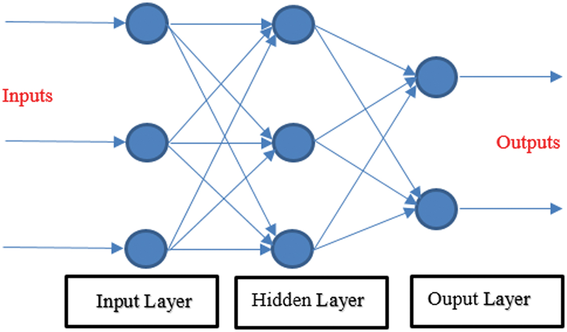 Fig. 1. Topology of a single-layer network with input, hidden, and output nodes.
In the present paper, the MLP feed-forward back propagation neural networks (FFBP) configuration of the ANN, as illustrated in Fig. 2, consists of a number of interconnected adaptive units (neurons), processed in parallel. Backpropagation neural network (BPNN) is a linear regression algorithm related to supervised learning, and it is a gradient descent technique adjusting the weights, minimizing the loss function via various activation functions, and improving the output’s metric (Electric Power, EP) accuracy. Hence, commonly used activation functions include the log-sigmoid (logsig) and the tan-sigmoidal (tansig), whereas for a more accurate forecasting of the EP, the superiority of tansig is designated. The input parameters considered are as follows: ambient pressure (AP), exhaust volume, ambient temperature (AT), and relative humidity (RH), while the EP represents the output variable of the CCPP power plant.
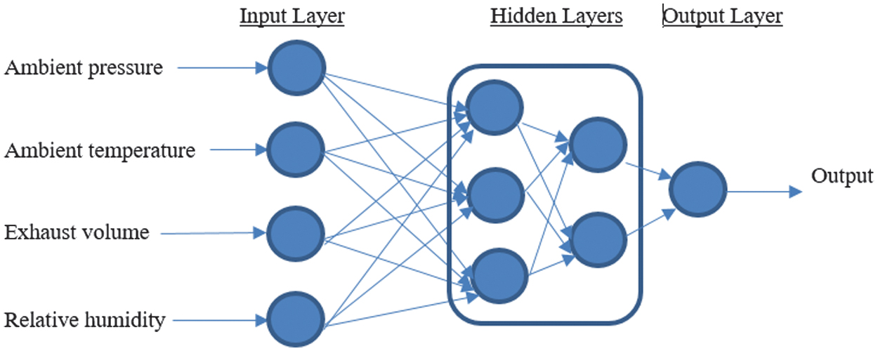 Fig. 2. MLP configuration of a BPNN with input, hidden layers, and an output layer.
The training process of the BPNN consists of a four-step procedure designed to improve the model’s performance iteratively. It begins with allocating initial weights, where the network’s weights and biases are randomly assigned to initiate the learning process. This is followed by adopting the feed-forward operation using gradient descent, where input data flow through the network, and gradient descent helps determine how the weights should be adjusted. The third step involves error propagation by implementing a loss function, which calculates the discrepancy between the predicted and actual outputs to evaluate model performance. Finally, the process concludes with updating weights and biases, using the computed errors to refine the model’s parameters and enhance its predictive accuracy.
Hence, small weight values are assigned in the feed-forward stage, forecasting the output design parameter. The respective error (loss function) runs back at the ANN, whereas the biases and the weights are adjusted, and the entire process continues till the weights are assigned at the loss error’s minimum value. The respective layers, illustrated in Fig. 2, are denoted as i the input layer, j the hidden layers, and k the output layer. The input training vector is expressed as A, whereas and the desired value vector is denoted with B, where The input layers i and the hidden layers j are linked via the weight and considering the output layer k, the respective hidden and the output layers are connected via Hence, the network is initiated using a small random signal , received by the input unit, and then it is transmitted to all the hidden layer units. Therefore, the sum is calculated via:
whereas is the bias design vector. In case the activation function (logsig) of a neuron is 1, their weights are defined as biases, and the logsig is expressed as [8]:Hence, the signal received from the activation function is redirected to the output layer, calculated from the equation below.
As illustrated in the following expressions, this final signal is multiplied by the cap S sub j k.
In case that all the output units in the output layer have received a signal from the hidden layers, the output unit error generated becomes:
whereas is the output unit error.The output unit error travels back via the hidden layers, where an identical error is calculated, and based on the results, the adjustments to these biases and the weights are given as:
where is the difference deduced when the error was fed back into the architecture through hidden layers:where is the learning rate, for .Therefore, the respective error between the predicted and the actual data is expressed using the MSE metric of the network’s performance as:
Incorporating neural networks led researchers to predict the CCPP performance under various maximum and operational base loads, such as deploying the transparent open box to predict output EP [9]. In the GTs field, the performance of a high-dimensional model representation coupled with an ANN is reliable [10]. The evaluation of a micro-GT’s performance under different weather conditions is presented [11]. Furthermore, a combined cooling, heating, and power plant for performance prediction [12] was used to validate the condition monitoring and diagnosis methodology of a combined heating and power plant [13]. The performance of an industrial GT, considering the RH, AP, and AT as input variables, with encouraging results after 10,000 epochs, is examined [14]. The regression method is used to model the baseline consumption of a combined heat and power plant and the EP prediction of a CCPP [15,16].
In power plants with multiple objectives, for the estimation of the output power of a coal-fired power plant as well as the thermal efficiency and the environmental effect [17–21], the modeling and optimization of a combined gas and steam (COGAS) power plant implementing a MLP model contribute to maximum efficiency [22]. The assumed heat rate of a COGAS power plant is an output parameter using three input parameters: the fuel gas heat rate (P1), the CO2 percentage (P2), and the power output (P3); this combination and redundancy achieved reliable outcomes [23].
This research shows how the power and performance of a CCPP increase by reducing the input design variables. The practicals started with 4 variables, slightly reduced them to 3, and then to 2. The study shows that using ANNs is the most efficient method for addressing the energy sector problem. A more detailed literature review evaluation of the AI approach and various ML techniques within the power sector with positive qualities is depicted in the following section.
III.LITERATURE REVIEW
ANNs are an efficient tool for the consideration of complex problems and have been adapted by several investigators worldwide for several real-world engineering problems in the solar [24] and in the solar power sector in islands [25]. In the power plant sector, various techniques for a number of input and output datasets have been proposed over the last few years, with robust outcomes. Therefore, for various thermodynamic input parameters, the power output forecasting of a CCPP is also forecasted [26]. The validity and reliability of the neural networks in a traditional GT power plant are studied by the AT impact on power generation and fuel consumption [27]. An interesting analysis of the single-shaft GT provided encouraging outcomes [28]. The control and performance analysis of a combined heat and power plant is studied [29]. The monitoring of the drum level of a traditional thermal power plant, adopting a BPNN method, was presented [30]. In the GT field, the prediction of the compressor’s performance map with the noise reduction of the measured data via neural networks, towards improving their operational quality, is studied [31]. In a steel thermal plant with implicated input variables, the advocacy of ANN efficiency over the autoregressive moving average exogenous time series model is underlined [32]. The overall attainment evaluation in a Western Balkan power plant under controlled modifications is proposed [33].
An interesting comparison between the MLP and the radial basis functions (RBF) networks for the fault analysis of the GTs is conducted, highlighting the superiority of RBF [34]. Furthermore, the implementation of neural networks to reduce unusual (indirect) losses in a thermal power plant is presented [35]. The short-term load forecasting in various types of power plants is depicted. Therefore, a hybrid model consisting of a fuzzy logic exergy model and a CCPP neural network contributed to robust solutions [36]. A hybrid model integrating a neural network with a genetic algorithm, selecting the optimum architecture via the trial-and-error process, improved the computational cost [37]. Adaptation of various deep learning methods, such as the single and fast neural networks, is also investigated for the EP estimation of a CCPP, with secured robustness [38]. A statistical inference prediction of the performance model with reliable outcomes and improved computational cost in the process is highlighted [39]. Various ML techniques for the monitoring process of a CCPP are also incorporated [40]. A multilinear regression ML methodology for an optimum predictive load estimator is achieved [41]. A decision-making tool of coherent complex data environmental control forecasting, utilizing AI, is validated [42].
A sensitivity analysis of the interpreted neural networks, jointly with various agnostic models, contributes to inspirational and productive results under full operating conditions [43]. In the combined cycle GT field, deep learning methodologies investigated the control optimization of its auxiliary components [44]. A comprehensive review of achieving efficient optimum solutions in various CCGT plants, incorporating an Adaptive Inference Neuro-Fuzzy logic system, is envisaged [45]. A novel ANN was employed for power output forecasting using an electrostatic discharge optimization technique [46]. A brief introduction of the gap’s closure contribution to knowledge, as well as the objectives of the present study, is envisaged in the following section.
IV.GAPS IN KNOWLEDGE, MOTIVATION, AND OBJECTIVES
In the present study, the primary interest is dedicated to CCPP plants, with the main target to model and to forecast their performance in terms of an MLP FFBP neural network for a multidimensional dataset (9568) under full loading conditions in Turkey [47]. These four parameters include the AT, exhaust volume (V), AP, and RH, to predict the EP, contributing to the upgrading of the computational performance of the CCPPs. Recently, there has not been enough contribution about the impact on the performance computation and the robustness by deducing various input parameters in the literature. This gap is filled by introducing a novel methodology of reducing the specific input design variables into 3 (AT, V, and AP) and 2 different combinations (AT and V, AT and AP, V and AP). Consideration of the RH, in the reduced input parameters due to meaningless outcomes, is omitted, and a comparison with identical studies will be pointed out. Another key contribution of this pioneering study is to deliver reliable and accurate deliverables regarding the network’s performance, forecasting the EP. Despite the reduction, this study ensures accuracy in predicting the attitude of CCPP modeling. This streamlining improves computational efficiency and uniquely contributes to the overall research.
Table I highlights the implementation of AI and ML techniques in traditional and hybrid combined power plants. Recently, many tools have been adopted to model and forecast the EP of CCPP plants. There is inadequate research on the selection and appropriate request of the cutting-edge tools, namely AI-based extrapolative models that can simulate nonlinear patterns in the CCPP. Hence, the entire trend is based on the premise that this investigation applied an MLP network structure of the reduced input features (3 and 2) of the neural network (FFBP) that is more robust and reliable on the existing dataset (9568), using novel findings and making a comparison with previous studies [16,23,29]. Furthermore, to the best of the authors' knowledge, MLP network techniques have not been fully utilized in previous power plant modeling studies. This new approach addresses the multidimensional handling of the novel reduced dataset to prevent power failure and stabilize its operation. The methodology used in the present study will be highlighted in the following section.
Table I. Concise overview of ANN techniques for boosting-related CCPP in literature
| Types of plants | Plants’ choice constraints | Types of ANN techniques | Responses | Remarks and issues on undersupplied | Findings | References | |
|---|---|---|---|---|---|---|---|
| 1 | CCPP | Ambient Temperature, Exhaust Vacuum, Ambient Pressure, Relative Humidity | Machine Learning Methods (MLAs) | CCPP hourly electric power prediction | Various MLAs, such as the kth-nearest neighbors (KNN), gradient-boosted regression rate (GBRT), Linear Regression (LR), ANN, and Deep Neural Networks (DNN), estimate the electric power output with significant outcomes, accurately. | Results show that the state-of-the-art surpasses GBRT in terms of predicting optimum electric output power (EP) | Siddiqui et al. [ |
| 2 | CCPP | Ambient temperature, Exhaust Vacuum, Ambient pressure, Relative humidity | Hybrid Machine Learning approaches | Power plant’s output power with the minimum waste | BOA combined with a PPE algorithm, BOAPPE, jointly with the SVM forecasted the output power of CCPP with robust solutions, avoiding technical issues on the power outage | BOAPPE methodology improved the convergence speed, avoiding the trapping into local optimum solutions | Wang et al., [ |
| 3 | Combined Cycle Gas Turbine Power Plant | Inlet temperature (flue), absorber column operating pressure, amount of exhaust recycled, and amine concentration | Taguchi Design of Experiment | Optimization of post-combustion CO2 capture | Monoethanolamine solvent, employed through the Taguchi design experimental method, mitigated the energy requirements of the system, studying the varying inlet flue gas temperature, the absorber column operating pressure, the exhaust gas recycle, and the amine concentration under statistical investigation. | The statistical optimization concept of the post-combustion capturing of CO2 is demonstrated. | Petrovic and Soltani [ |
| 4 | Natural gas-fired combined cycle power plant | Flue gas emissions dataset between 2011 and 2015 | Hybrid Machine Learning method | Power plant’s NOx emissions prediction | ANFISGA strategy evaluated accurately the NOx emissions at the minimum error, with a positive impact on the CCPP performance, resolving the environmental and the society’s needs | The impact of the coupled GA with ANFIS provided optimum solutions | Dirik [ |
| 5 | Gas Turbines Combined Cycle Power Plant | Dynamic optimal set point for the regularization level | Hybrid Machine Learning technique | Power plant’s efficiency forecasting | An integrated Fuzzy Logic model with a Genetic Algorithm (GA) predictive supervisory controller accurately evaluated the power plant’s performance, reducing the plant’s nonlinear effects. | The coupled fuzzy (GA) logic controller optimizes GTCCPP performance solutions. | Saez, Mila, and Vargas [ |
| 6 | CCPP boiler | Input data are selected by means of a sensitivity analysis | Machine Learning approaches (MLAs) | CCPP boiler performance | A cluster of optimum Taguchi-Sugeno Fuzzy Logic models (FL) successfully derived the CCPP’s efficiency and the tackling via a Chen series sensitivity method of the nonlinearities associated with the boiler’s operation. | The economic optimization of the plant in terms of the nonlinear FL model and the superheated steam pressure via the linear FL model | Seaz and Zuniga [ |
| 7 | CCPP | Ambient Temperature, Exhaust Vacuum, Ambient Pressure, Relative Humidity | Hybrid ML Technique | CCPP hourly output power estimation | An integrated MLP topology of a neural network (ANN) model with a Genetic Algorithm (GA), towards the accurate electric power output estimation, increasing the regression R values of the network (reliability and robustness), compared to identical studies. | Results for the optimum MLP architecture show that the root mean square error (RMSE) reaches a value of 4.304, substantially lower than the available MLPs in the literature, but higher than several complex algorithms, such as the KStar and the Tree-based algorithms. | Lorencin, Mrzljak, and Car [ |
| 8 | CCPP | Ambient Temperature, Vacuum Exhaust, Ambient Pressure, Relative Humidity | Machine Learning Approaches (MLAs) | CCPP output power full load forecasting and anomaly detection. | Full load estimation of the power output using several machine learning algorithms, such as Linear Regression (LR), Support Vector Machines (SVM), Random Forests (RF), and neural networks (ANN), contributing to the reduction of the anomalies and the operation’s detection of a CCPP power plant | Results show that the superiority of the Random Forest (RF) technique by means of the highest accuracy using less than half of the 10,000 dataset points, while the unsupervised algorithms identified sparse synthetic anomalies of 1.5 % from the entire dataset | Hundi, Shahsavari [ |
| 9 | CCPP | Ambient Temperature, Vacuum Exhaust, Ambient Pressure, Relative Humidity | A stacking prediction method, based on a multi-model ensemble, and a traditional machine learning method, such as the Random Forest (RF) | An efficient and reliable CCPP power output under full conditions prediction model | Full load evaluation of the power output from a CCPP plant, implementing a stacking ensemble optimization algorithm, compared with the conventional Machine Learning algorithm (RF) and other ensemble methods cited in the literature to address the accurate planning of the electricity generation and utilization | The results demonstrate a high prediction robustness of the power output, under multiple complex environmental variables, designating its superiority, in terms of various machine learning methods such as the Random Forest (RF) and additional ensemble methods | Qu et al. [ |
| 10 | NGCCP | Effective use of underground resources such as natural gas | Life performance models such as FL and ANN | Power output estimation was carried out | Full loading conditions power output prediction comparing FL and ANN models, addressing the life performance forecasting via underground resources such as natural gas. | Results depict that the relative error estimation via FL varies between 0.59 % – 3.54 % and via ANN varies between 0.001% – 0.84 %, illustrating the neural networks’ advocacy | Karacon et al. [ |
V.METHODOLOGY
ANN can handle complex information, moving towards understanding the choice from the CCPPs [3]. Therefore, the primary objective is to leverage ANNs to forecast plant performance in terms of EP. The CCPP comprises a GT, a steam turbine, and a heat recovery steam generator, as illustrated in Fig. 3. In a CCPP, a GT produces hot gases and outputs EP. These gases from the GT pass over a water-cooled heat exchanger, generating steam, which is used to produce output power (EP) with the aid of the steam turbine coupled with generators. An extended description of a CCPP’s operation can be found in [5,6]. In addition, the feature to evaluate the multiple input contrast and hidden layer functions allows a detailed analysis of the interdependencies among the input features, using the AT, exhaust vacuum, AP, and RH on the power output. Therefore, the neural networks handle the regression tasks with ease. Furthermore, it justifies its selection for achieving efficient and timely predictions in this research study. The MATLAB neural network toolbox (nntool) facilitates the exhaustive simulation part to be compared with reliable online datasets [47]. The main metrics to be explained are the test and the performance of the entire dataset, followed by a brief description below.
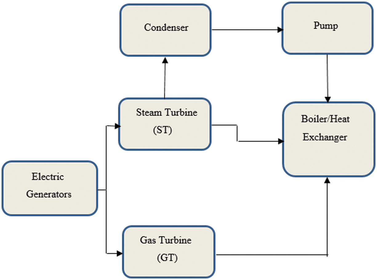 Fig. 3. Functional diagram of a CCPP power plant.
A.DATASET PREPARATION
The CCPP dataset consists of 9568 non-stationary points received from a gas-fired power plant with a 420 MW capacity in Turkey for 6 years from 2006 to 2011 [47]. The respective input features involved in this procedure are the AT, exhaust vacuum (V), AP, and RH, while the output forecasted variable is the EP. This primary dataset comprised 674 datasets in .xls format for a daily representation, although a few noisy and incompatible datasets were included. After some preprocessing steps, these conflicting and noisy points were rejected due to the disturbance interference. The primary aim of this study is to make a deep comparison of the various datasets’ network performances. Thus, the following section presents an overview of the dataset, depicting a sample of the input and the output parameters to be considered, as Table II illustrates. Therefore, the novel capabilities of reducing the input parameters into 3 (AT, V, AP) and the different combinations into 2 (AT and V, AT and AP, V, and AP), as explained in section II, contribute to this direction [47]. The primary goal of the testing is to evaluate the reduced dataset, which includes both input and output features. According to the MATLAB Neural Network Toolbox (nntool) [48], the dataset is by default divided into 75% for training, 15% for testing, and 15% for validation. This partitioning is done while considering the limited CPU resources, as shown in Fig. 4. In this study, despite the massive amount of data, there is no reduction in the training, testing, and validation subsets, and the setting of the entire procedure before the simulation is examined later.
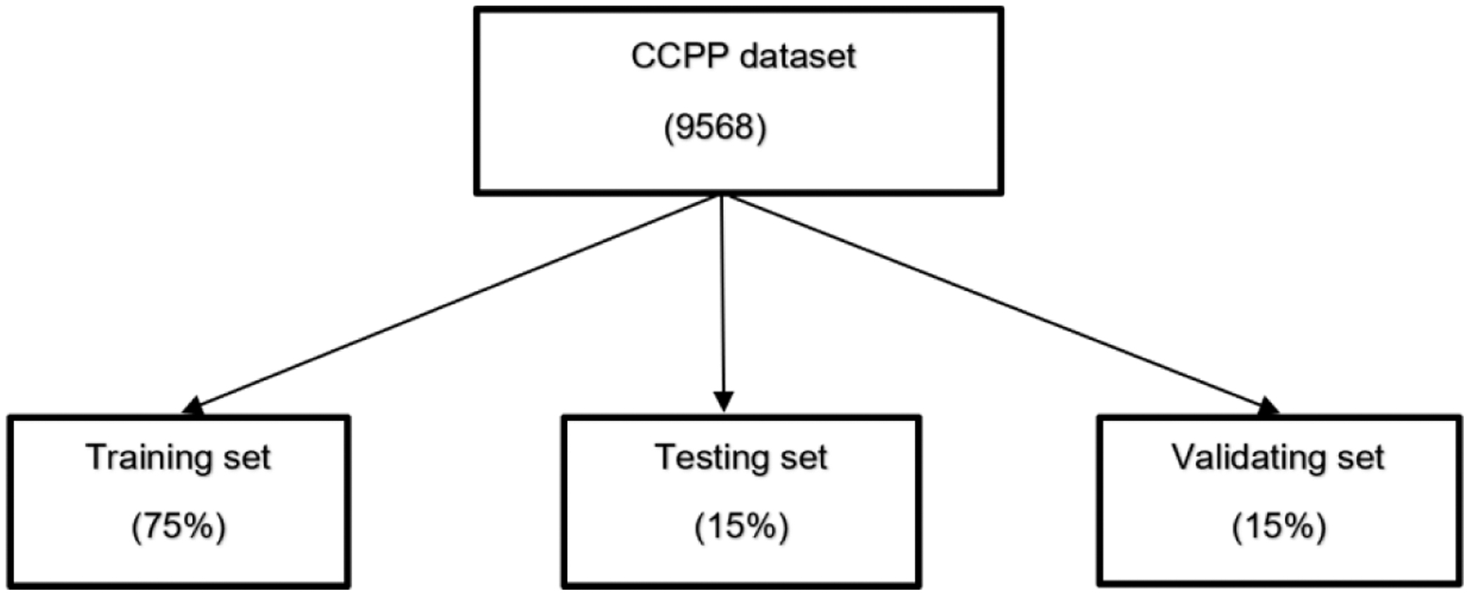 Fig. 4. Percentage sampling of the CCPP entire dataset (9568) in training, testing, and validating.
Table II. Actual data were taken from a CCPP [47]
| Sample | AT (Input) (°C) | V (Input) (cmHg) | AP (Input) (mbar) | RH (input) | EP (output) (MW) |
|---|---|---|---|---|---|
| 1 | 9.34 | 40.77 | 1010.94 | 90.01 | 490.48 |
| 2 | 23.64 | 59.49 | 1011.4 | 74.2 | 445.75 |
| 3 | 29.74 | 56.9 | 1007.15 | 41.91 | 439.76 |
| 4 | 19.07 | 49.69 | 1007.22 | 76.79 | 452.09 |
| 5 | 11.8 | 40.66 | 1017.12 | 97.2 | 464.43 |
| …. | ……. | ……. | ……. | ……. | |
| 9565 | 16.65 | 49.69 | 1014.01 | 91 | 460.03 |
| 9566 | 13.19 | 39.18 | 1023.67 | 66.78 | 469.62 |
| 9567 | 31.32 | 74.33 | 1012.92 | 36.48 | 429.57 |
| 9568 | 24.48 | 69.45 | 1013.86 | 62.39 | 435.74 |
B.THE SETTING OF THE NETWORKS
A FFBP is implemented in the MLP structure of the present neural network, implementing a Levenberg–Marquardt (LM) training algorithm, considering the MSE as the performance metric. The theoretical background of LM is beyond the scope; thus, it is omitted. The learning function has changed the weight between the neurons by implementing the FFBP algorithm [21]. Furthermore, the adopted activation function in this study is the tansig for robustness reasons. The input and output parameters for the reduced number of parameters (2, 3) are illustrated in Table III. An architectural sample network model of two input parameter combinations (I, P1+P2) identical for the (P1+P3, P2+P3) with two hidden layers (H) of two and one neuron, including an output parameter (EP), is illustrated in Fig. 5.
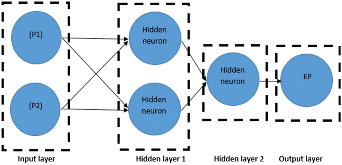 Fig. 5. ANN structure model for two input parameters (P1+P2).
Table III. Input and output variables of the ANN model
| Term notation | Variable description | Output power |
|---|---|---|
| Two | P1+P2 | AT (°C) and V (cmHg) EP |
| P1+P3 | AT (°C) and AP (mbar) EP | |
| P2+P3 | V (cmHg) and AP (mbar) EP | |
| Three | P1+P2+P3 | AT (°C), V (cmHg), and AP (mbar) EP |
Figure 6 designates the combined model with the three input variables (P1+P2+P3) with two hidden layers (H) of three and one neurons (nodes), as well as an output parameter (EP), whereas the output parameter corresponds to the output EP.
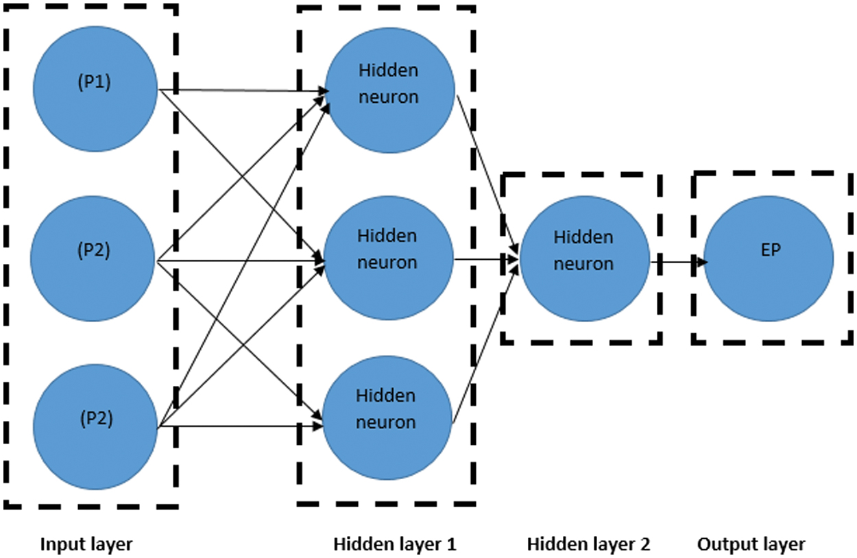 Fig. 6. ANN structure model for three input parameters (P1+P2+P3).
C.FLOWCHART OF THE PROPOSED ARCHITECTURAL MODEL
The proposed training, testing, and validation process for the LM training algorithm of the reduced input features into the combined 2 and 3 of the current test case with 10,000 epochs and 1000 validation steps is presented in Fig. 7. Therefore, the loop with respect to the two and the three input parameters is currently assumed.
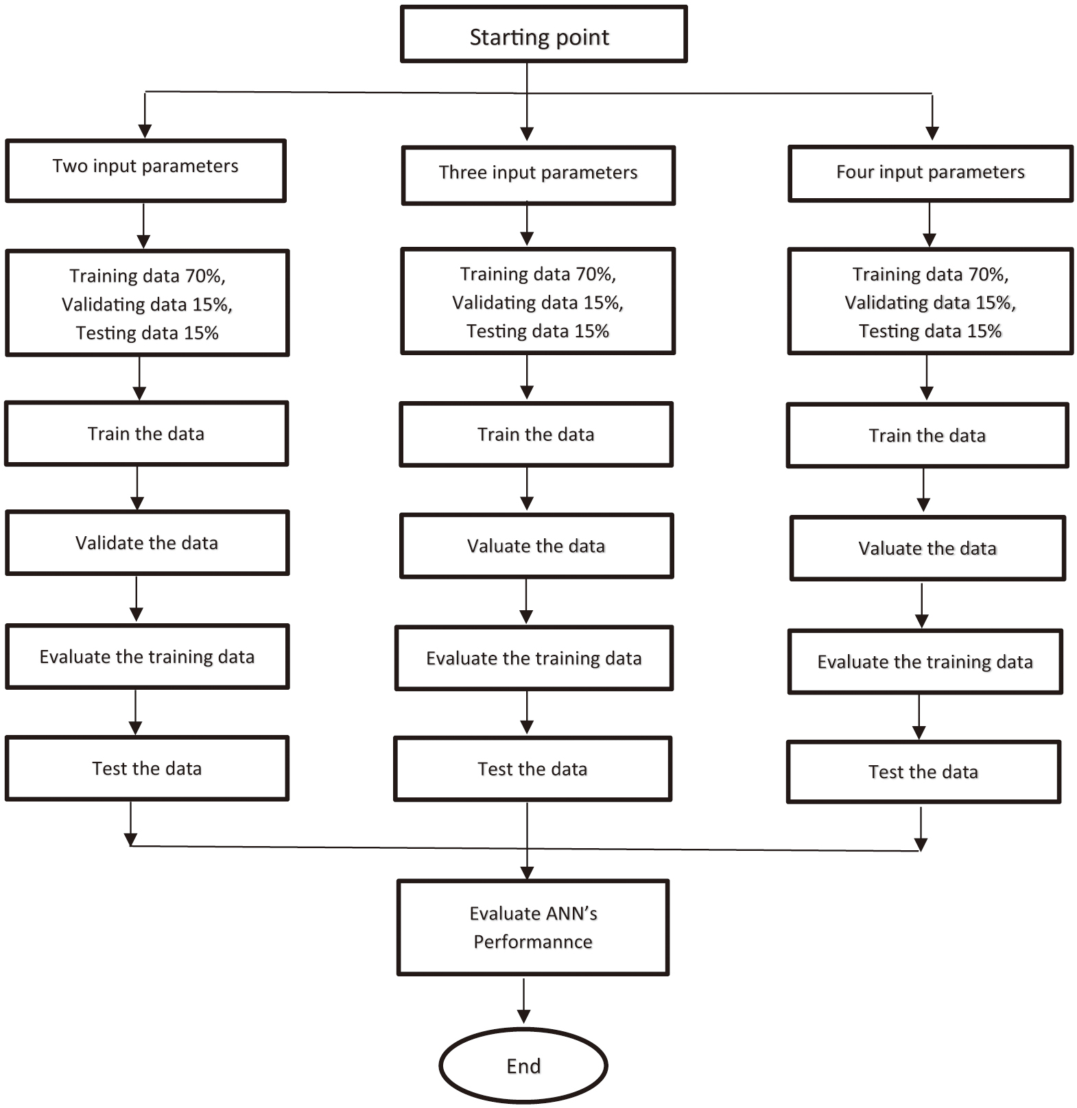 Fig. 7. Flow process of the present study.
The network is constructed using the neural network’s architecture, including the neurons, layers, training function (LM), and the learning algorithm (tansig). The neural network architecture for the present study is configured automatically with MATLAB software’s graphical user interface capabilities [48]. Further investigation to amend the dataset percentage regarding the training/testing/validation principle is not considered for novelty reasons. The sensitivity and reliability of the outcomes after reducing the input parameters from four have been investigated [6]. Additionally, the combination of two input features has also been explored in studies [16,23,29], yielding interesting and reliable results, as explained below.
VI.RESULTS AND DISCUSSION
The analysis of the results with a few concluding remarks is envisaged in this section, forecasting the output power of a fully operational CCPP plant, through the reduced number of combinations of two input parameters (P1+P2, P2+P3, P1+P3) and of three input parameters (P1+P2+P3). Each design variable from the combined input variables (P1+P2, P2+P3, P1+P3) presents a different impact on the output parameter (EP). Hence, each of the three parameters (AT, V, AP) was examined for the respective data size (9568) (70% training, 15% validation, 15% testing) for 20 hidden layers. These settings for the respective number of simulations are depicted in Table IV. The training algorithm LM was adopted for the whole procedure, and its theoretical background is beyond the scope, thus excluded, and more information can be found in the literature. The respective network’s testing and performance database is expressed in terms of the MSE. A sample geometry of the network of the two input combined variables (P1+P2, P2+P3, P1+P3) with 20 hidden layers as well as an output layer, is shown in Fig. 8. After the respective settings, the training process adapting the LM of MATLAB neural networks nntool [48], contributes to the achievement of robust outcomes for a different number of hidden layers, which are discussed below.
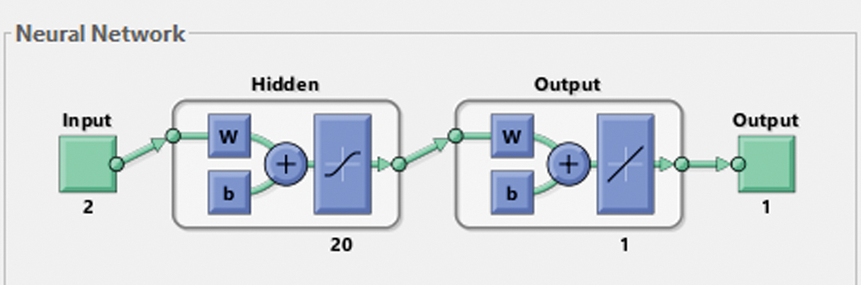 Fig. 8. Sample geometry network structure with two input variables for 20 hidden layers [48].
Table IV. Settings of the design variables of the combined two parameters
| Data size | 9568 |
| Applied variables | AT and V, V, and AP, AT and AT and AP |
| Hidden layers | 20 |
| Training Function | Levenberg–Marquardt (LM) |
| Number of epochs | 1000 |
A.LEVENBERG-MARQUARDT ALGORITHM TRAINING WITH 2 PARAMETERS (P1+P2, P1+P3, P2+P3)
Figures 9–11 depict the failure of reaching the given number of epochs (1000) by means of the maximum validation allowance of the (LM) toolkit, of the combined parameters (P1+P2, P1+P3, P2+P3) reaching 53, 24, and 79 epochs.
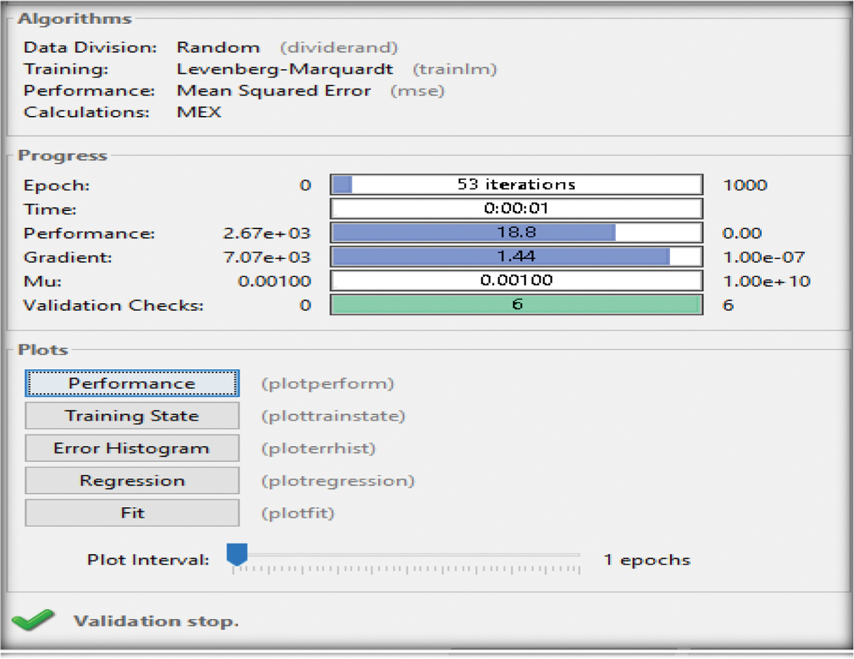 Fig. 9. Training outcome of the two input parameters (P1+P2) [48].
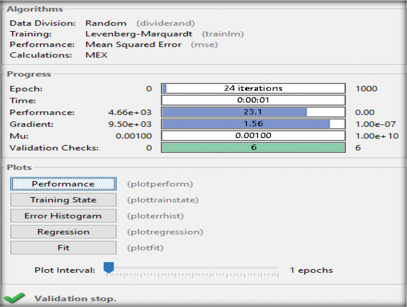 Fig. 10. Training outcomes of the two input parameters (P1+P3) [48].
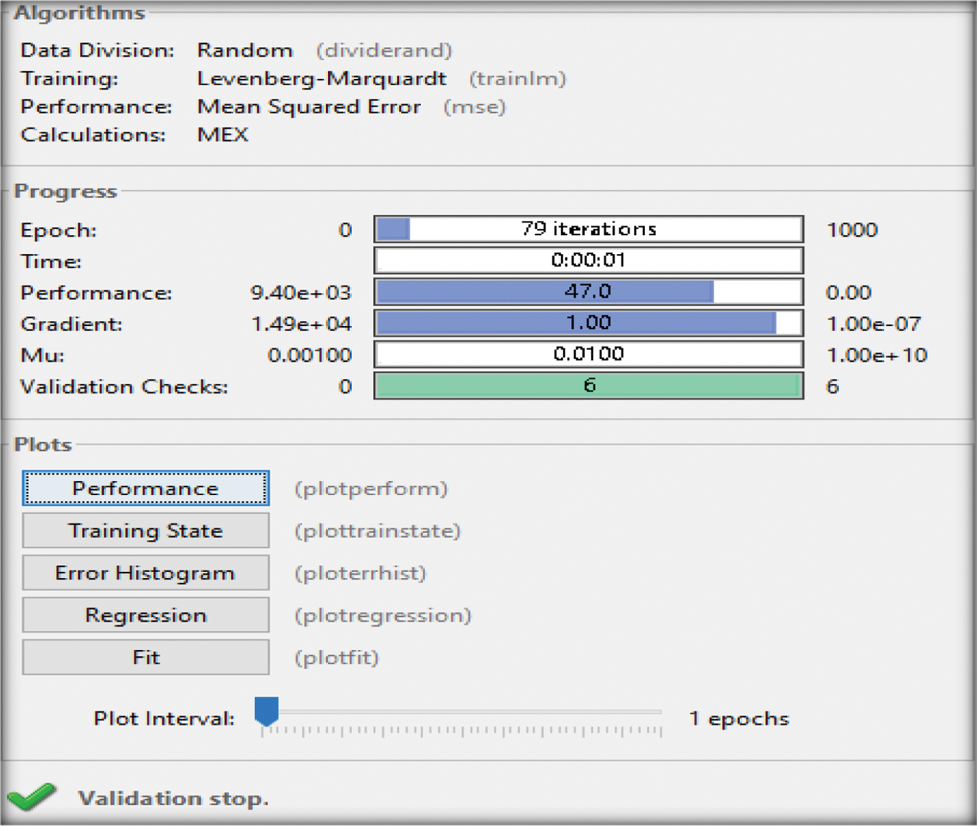 Fig. 11. Training outcomes of the two input parameters (P2+P3) [48].
The regression coefficient R (correlation) for the training, validating, and the testing of the combined parameters [P1+P2, P1+P3, and P2+P3] presents R regression values of 0.967, 0.966, and 0.965 shown in Figures 12–14, with almost excellent fitting (R=1) between the target and the actual dataset towards robustness as well as very good quality of the networks. The advocacy of the (P1+P2) configuration with computational benefits is also presented.
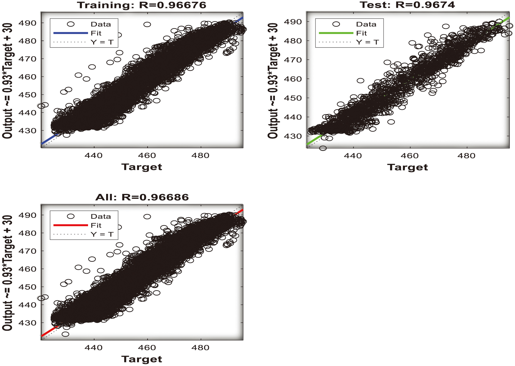 Fig. 12. Regression analysis outcome for (P1+P2) input parameters [48].
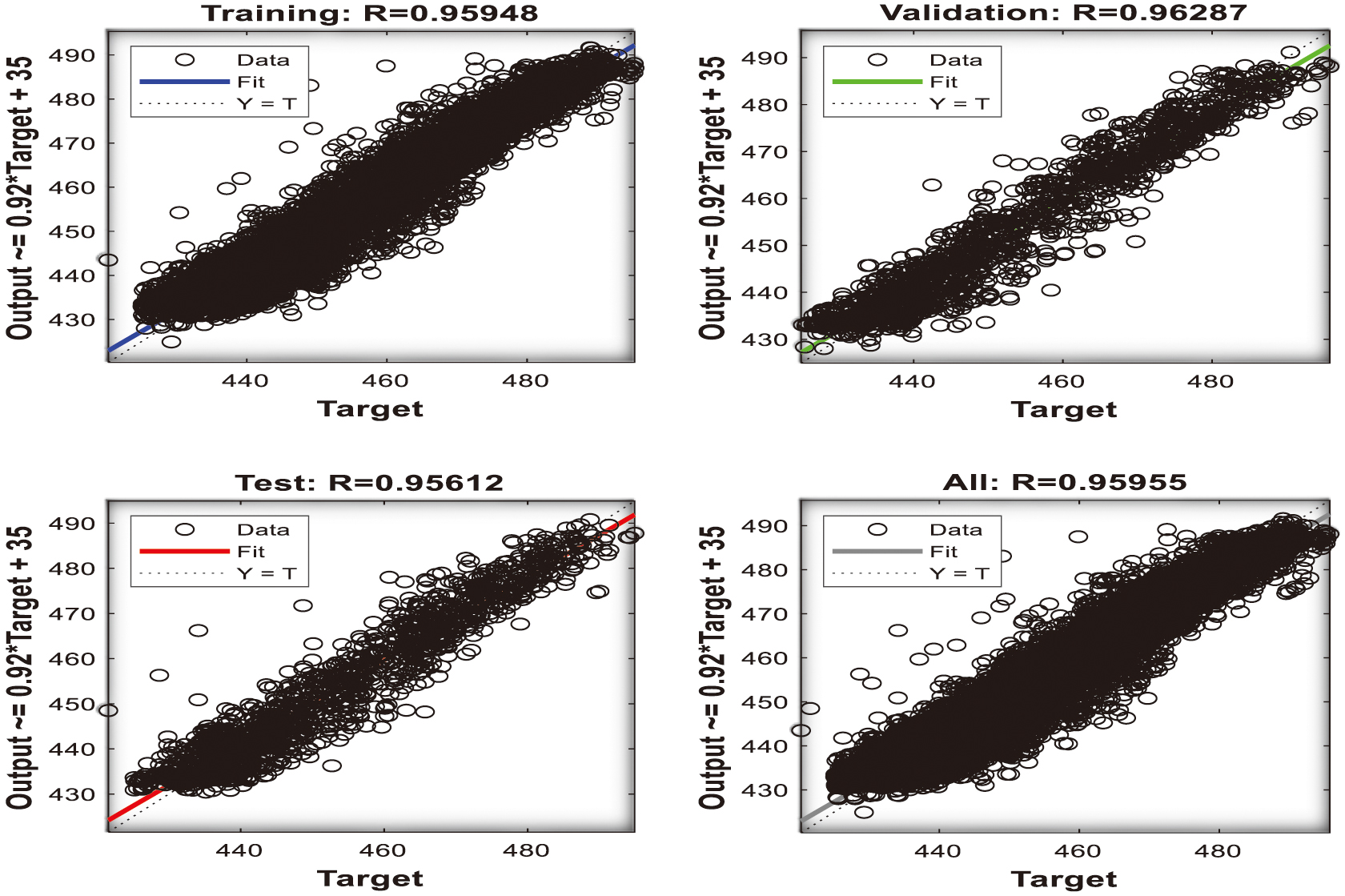 Fig. 13. Regression analysis outcome for (P1+P3) input parameters [48].
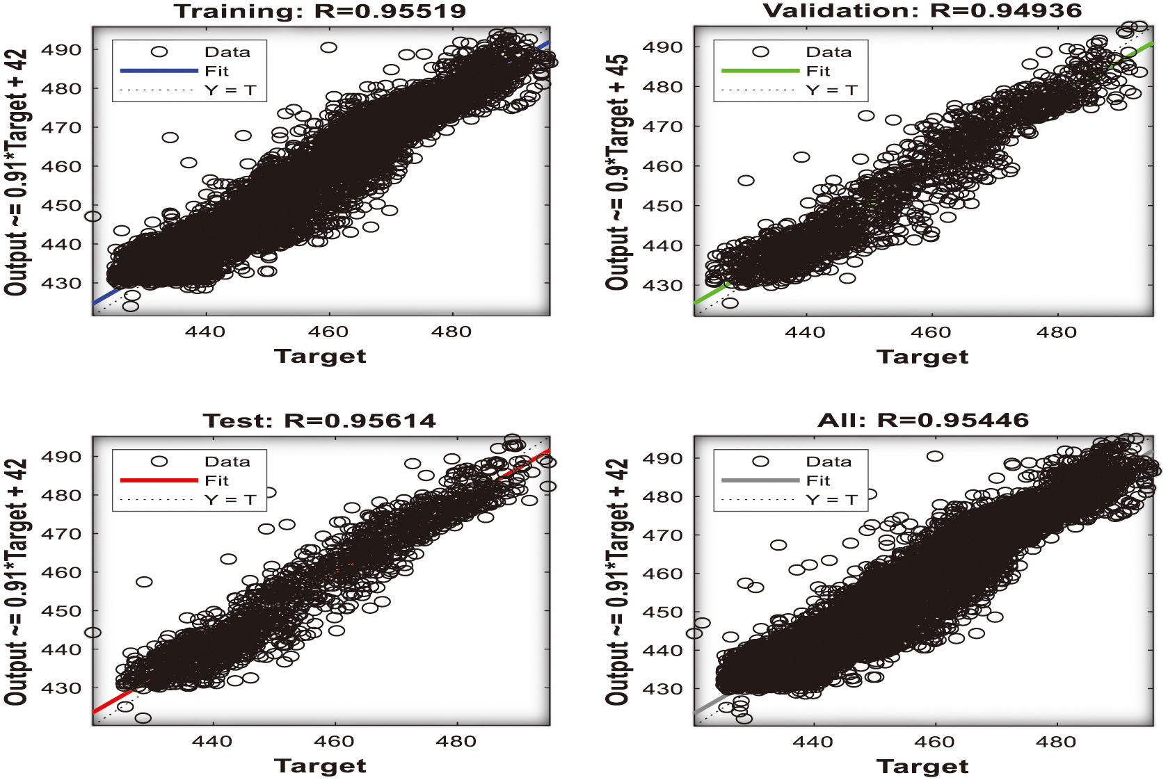 Fig. 14. Regression analysis outcome for (P2+P3) input parameters [48].
Tables V–VII illustrate an impact on the network’s quality and performance for a different number of neurons (hidden layers), using the two combinational (P1+P2, P1+P3, P2+P3) design variables with reliable results. The same argument of the best-performing network for (P1+P2 and P1+P3) employing the MSE is depicted for 500 hidden layers, while the worst network is designated for 100 hidden layers. A different outcome exists for the final (P2+P3) combination since the maximum and the minimum performance metrics occur for neuron sizes 10 and 500. Table VIII illustrates the superiority of the (P1+P2) network with respect to the lowest (improved) MSE metrics. The network’s accuracy and performance results considering incorporating a third parameter (P1+P2+P3) are shown below.
Table V. Neuron’s impact of the (P1+P2) parameters for the LM training algorithm
| Hidden layers | Training performance | Validation performance | Training regression | Validation regression | Test regression | Stopping criterion | Iteration | Best epoch |
|---|---|---|---|---|---|---|---|---|
| 10 | 18.9523 | 20.2356 | 0.967221 | 0.96454 | 0.96791 | “ | 41 | 25 |
| 20 | 16.8597 | 20.1873 | 0.967392 | 0.96415 | 0.96779 | “ | 53 | 47 |
| 50 | 18.2058 | 19.3837 | 0.967751 | 0.96595 | 0.96784 | “ | 64 | 58 |
| 100 | 17.3405 | 24.7622 | 0.970112 | 0.96775 | 0.96595 | “ | 13 | 7 |
| 200 | 17.2695 | 18.7923 | 0.970056 | 0.96740 | 0.96557 | “ | 14 | 8 |
| 500 | 15.3367 | 21.0806 | 0.970157 | 0.96117 | 0.94507 | “ | 14 | 8 |
Table VI. Neuron’s impact of the (P1+P3) parameters for the LM training algorithm
| Hidden layers | Training performance | Validation performance | Training regression | Validation regression | Test regression | Stopping criterion | Iteration | Best epoch |
|---|---|---|---|---|---|---|---|---|
| 10 | 23.2854 | 22.2311 | 0.958382 | 0.957741 | 0.9532210 | “ | 30 | 15 |
| 20 | 23.1867 | 22.1193 | 0.967392 | 0.962874 | 0.9561121 | “ | 24 | 18 |
| 50 | 23.3592 | 23.9369 | 0.960500 | 0.957741 | 0.9597410 | “ | 64 | 58 |
| 100 | 22.1767 | 22.0989 | 0.961537 | 0.960790 | 0.9565150 | “ | 13 | 7 |
| 200 | 21.6054 | 22.4459 | 0.961978 | 0.960706 | 0.9612210 | “ | 14 | 8 |
| 500 | 20.6423 | 27.0140 | 0.965851 | 0.952698 | 0.9558010 | “ | 14 | 8 |
Table VII. Neuron’s impact of the (P2+P3) parameters for the LM training algorithm
| Hidden layers | Training performance | Validation performance | Training regression | Validation regression | Test regression | Stopping criterion | Iteration | Best epoch |
|---|---|---|---|---|---|---|---|---|
| 10 | 48.2331 | 47.6512 | 0.913200 | 0.911620 | 0.9132300 | “ | 92 | 86 |
| 20 | 47.0158 | 48.7354 | 0.915440 | 0.913800 | 0.9208900 | “ | 79 | 73 |
| 50 | 45.0213 | 49.2521 | 0.920610 | 0.911500 | 0.9153100 | “ | 35 | 31 |
| 100 | 43.0685 | 49.4849 | 0.923340 | 0.908230 | 0.9129800 | “ | 17 | 11 |
| 200 | 39.1248 | 45.5741 | 0.930450 | 0.913420 | 0.9263200 | “ | 29 | 33 |
| 500 | 35.5872 | 55.2711 | 0.940160 | 0.902310 | 0.9711180 | “ | 16 | 10 |
Table VIII. Lowest MSE values for the input parameters (P1+P2, P1+P3, and P2+P3)
| Input parameters combinations | Mean square error |
|---|---|
| P1+P2 | 15.3367 |
| P1+P3 | 20.6423 |
| P2+P3 | 35.5872 |
B.RESULTS WITH THREE INPUT VARIABLES (P1+P2+P3)
The addition of another variable (datasets AP, P3) to the settings of the design parameters is summarized in Table IX, and a sample network topology with 20 neurons is also illustrated in Fig. 15.
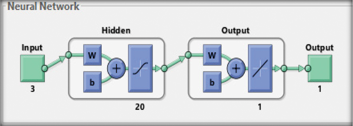 Fig. 15. Network geometry with three input parameters for 20 hidden layers [48].
Table IX. Settings of the design variables of the combined three parameters
| Data size | 9568 |
| Applied variables | AT, V, and AP |
| Hidden layers | 20 |
| Training function | Levenberg–Marquardt (LM) |
| Number of epochs | 1000 |
Figure 16 designates the training process setting of the LM algorithm for the (P1+P2+P3) input characteristics, whereas the neural network toolbox again fails to execute the entire number of epochs (1000), reaching 27 iterations. Figure 17 provides an estimation of the regression analysis R with a very good fitting between the actual and the target data for a value of 0.971, almost approaching an excellent value of 100%.
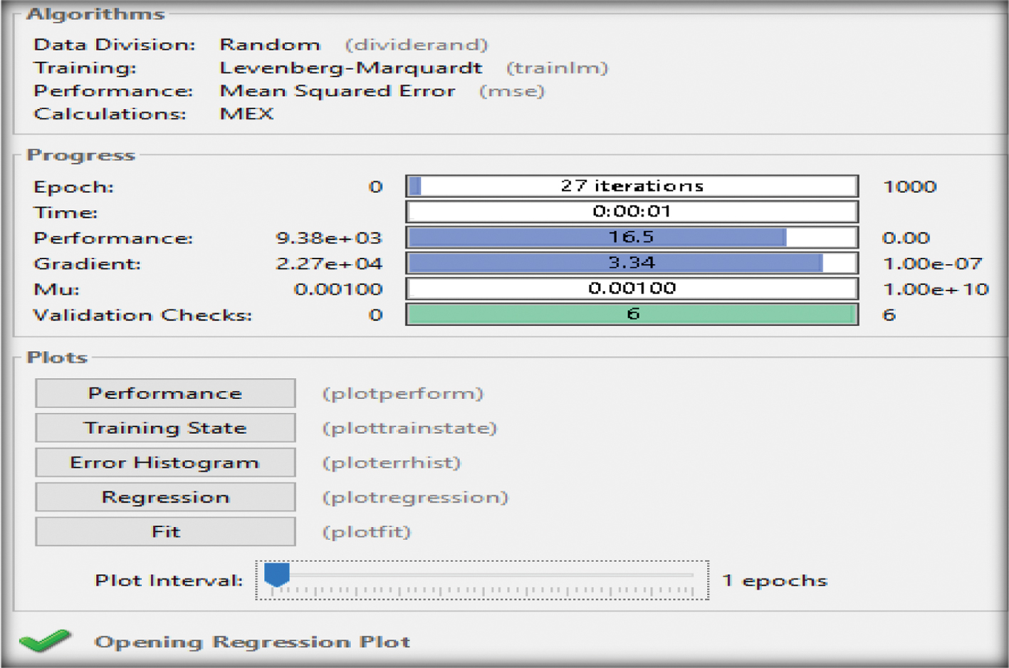 Fig. 16. Training outcome of the three input parameters (P1+P2+P3) [48].
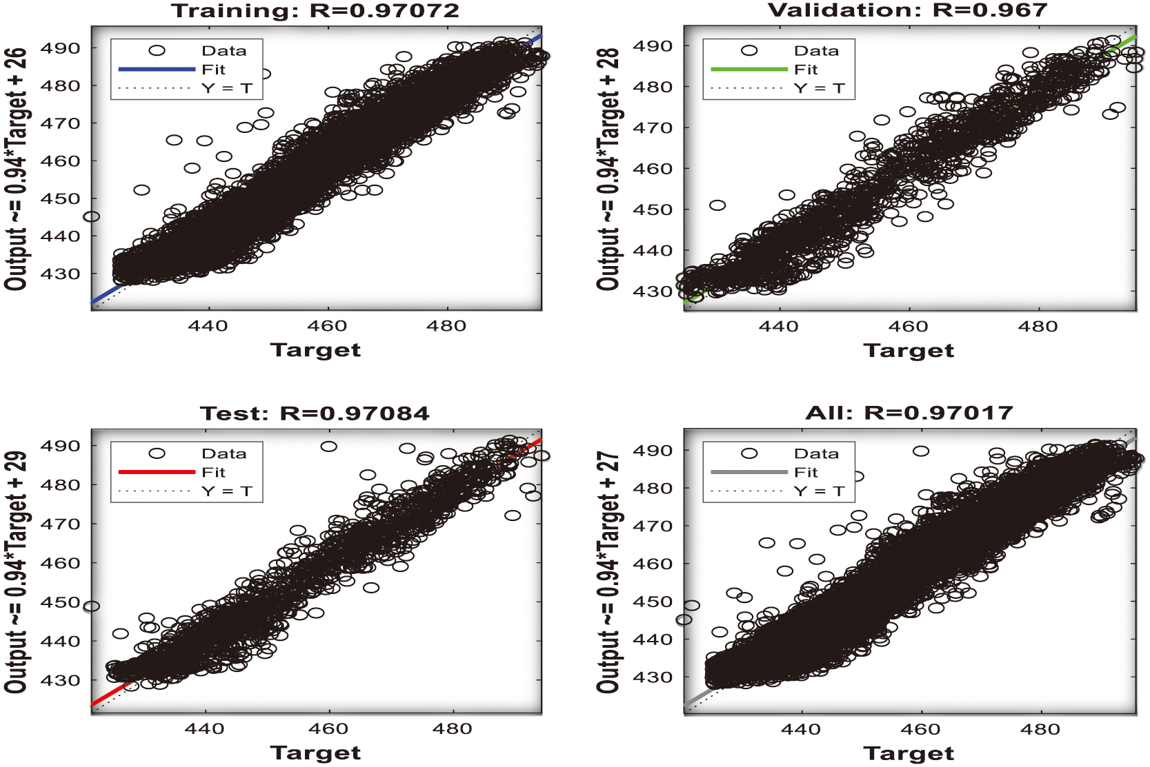 Fig. 17. Regression analysis of (P1+P2+P3) outcomes [48].
Table X illustrates the impact on the network’s structure and precision for the different sizes of the hidden layers, highlighting that the best network performance is achieved for 200 hidden layers and the worst for 20 hidden layers. Table XI presents a comparison between the performance of the MSE values of the two design variables combined dataset (P1+P2, P1+P3, P2+P3) and the three design variables (P1+P2+P3), forecasting the supremacy of the three input parameters. The process of deducting the four design variables into the combined two (P1+P2, P1+P3, and P2+P3) and the three (P1+P2+P3) contributes to reliable outcomes comparable to identical studies of conventional CCPPs (CHP, CCPP) [16,23,29]. This exciting agreement illustrates the superiority of using the (P1+P2+P3) setting in terms of the regression coefficient values (R), since it reaches a higher value of 0.9710, compared to the two combined design variables (P1+P2, P1+P3, P2+P3). Therefore, the proposed technique is more accurate and validated.
Table X. Neuron’s impact of the (P1+P2+P3) parameters for the LM training algorithm
| Hidden layers | Training performance | Validation performance | Training regression | Validation regression | Test regression | Stopping criterion | Iteration | Best epoch |
|---|---|---|---|---|---|---|---|---|
| 10 | 16.5213 | 18.0634 | 0.970212 | 0.967322 | 0.971224 | Validation Stops | 30 | 22 |
| 20 | 16.6797 | 19.0852 | 0.970173 | 0.967000 | 0.970844 | “ | 27 | 21 |
| 50 | 15.3994 | 16.3332 | 0.970391 | 0.971043 | 0.968232 | “ | 76 | 70 |
| 100 | 14.9842 | 15.9373 | 0.970646 | 0.972145 | 0.968832 | “ | 18 | 12 |
| 200 | 14.3761 | 16.7281 | 0.970887 | 0.971041 | 0.972278 | “ | 14 | 8 |
| 500 | 13.8389 | 17.2457 | 0.971012 | 0.971210 | 0.964595 | “ | 13 | 7 |
Table XI. Comparison of the lowest MSE values of the two and the three input parameters
| Input parameter combinations | Mean square error |
|---|---|
| P1+P2 | 15.3367 |
| P1+P3 | 20.6423 |
| P2+P3 | 35.5872 |
| P1+P2+P3 | 13.8389 |
The combination of the two input parameters dataset (P1+P2, P1+P3, P2+P3) provides accurate and reliable solutions and the best prediction of the EP, identifying the superiority of the first dataset (P1+P2) in terms of the regression analysis R outcomes and the electric energy prediction (EP). None of these datasets met the requirements of satisfying the maximum number of validation checks (1000 iterations) and the performance metric regarding the MSE of validations and training process values, which again depicts the advancement of the first dataset (P1+P2). These solutions can be more accurate in encouraging and predicting the desired dataset. Moreover, these MSE and R values are slightly improved compared to other studies [16,23,29], of the best two combinational sets (P1+P2) and the three input variables (P1+P2+P3) dataset, depicting the novelty of the present study as highlighted in Table XII. Furthermore, with the redundancy of the design variables into three and two combined datasets, the multidimensional data accurately evaluates the output parameter (EP) at the minimum computational cost, which is beneficial for future applications [21]. Therefore, the ANN validates, to the greatest extent, its application in the energy field to provide reliable outcomes in terms of improved power performance with additional benefits in this exciting sector [15].
Table XII. Comparison of the MSE and R values with previous studies [16,23,29]
| Input parameters | MSE values | R values | MSE values | R values | MSE values | R values | MSE values | R values |
|---|---|---|---|---|---|---|---|---|
| P1+P2 | 15.3367 | 0.9701 | 16.3671 | 0.9681 | 16.4524 | 0.9652 | 14.5416 | 0.9648 |
| P1+P2+P3 | 13.8389 | 0.9710 | 14.2313 | 0.9694 | 14.2613 | 0.9686 | 14.4492 | 0.9655 |
VII.CONCLUSIONS
The EP output of a 210 MW CCPP in Turkey is modeled using regression analysis through an ANN. The approach is based on a novel methodology that reduces the original four design variables to combined input datasets, specifically, pairs (P1+P2, P1+P3, P2+P3) and the trio (P1+P2+P3), for performance evaluation. Therefore, MATLAB neural network (nntool) is the main adopted tool with a reliable setting and a very good impact on the network’s efficiency. Interesting and reliable outcomes for different sizes of the datasets have already been produced by several investigators, and the novelty in this study is the improved MSE values for the (P1+P2) parameters as well as the (P1+P2+P3) of (15.3367, 13.8389), including their higher correlation values of (0.9701, 0.9710), compared to the respective numeric from past studies as Table XII depicts [16,23,29]. Moreover, the randomness of the reduced data is illustrated in each training procedure employing the initial weights and bias values. The impact on the network’s performance of the increasing number of hidden layers for the reduced input parameters (2 and 3) test cases led to elaborating outcomes through the network’s quality for a large number of neurons (500). The authentic R regression values are accomplished, showing a perfect match between the target and the actual data.
By means of the numeric, the following conclusions were arrived:
- ▪Implementing the three different datasets (P1+P2, P1+P3, P2+P3) of the two combined input parameters predicts the EP with the following improved R regression values of 0.9701, 0.9658, and 0.9401, for the highest performance network of 500 neurons.
- ▪The combination of the dataset using two input parameters (P1+P2) configuration predicts the output metric (EP) at an improved MSE, compared to the other two parameters (P1+P3), (P2+P3) related networks, as Table XI illustrates.
- ▪The combination of the three input parameters (P1+P2+P3), is more reliable and robust than the two input datasets’ superior (P1+P2) configuration by means of accuracy and fidelity, since the regression value R reaches 0.9710. Hence, the positive impact on its quality is enhanced.
- ▪Adaptation of the LM training algorithm secures accurate solutions and fast simulations, a very beneficial constraint. However, the current study does not consider the other related training codes (BR and SCG).
Despite the simplicity of the technique, reliable solutions are entirely provided for the forecasting of EP. In implementing a lower dataset size, there is no guarantee that the performance will not be influenced because ANN can optimize and increase the network’s performance. The adopted dataset of the reduced design variables is reliable without missing any values or outliers because any duplication impacts the performance of the chosen model. According to the performance metric, this approach presents accurate performance outcomes at a lower cost. The validity of the neural networks MATLAB toolbox provides accurate and novel outcomes, replacing other modeling tools to solve identical real-world problems due to the lack of complex mathematical calculations and the privilege of providing robustness and inexpensive computations.