JAIT

I.INTRODUCTION

According to a survey, the only use of AI in psychiatry is for algorithm development, with no consideration for real-world interaction. There are still concerns about sample size, potential bias, absence of assessment, and possible difficulties in determining the ground truth, even though the obtained accuracy values are high and appear to support its use [1]. However, a study in psychology cases challenges Bayesian learning for theoretical reasons, namely fundamental hypotheses and assumptions that are rarely clarified and put to the test through experimentation [2].

The dynamism of the social environment has a big impact on psychological diseases. Environmental changes and progress over time can change social behavior, resulting in changes in patterns. This change in pattern has an impact on changes in symptoms that determine the classification of mental illness. One of the mental disorders that needs special attention in the current era is gaming disorder (GD).

Based on measuring tools obtained from addiction experts, currently, GD has 44 symptoms that can be used for early detection of GD adapted from the symptoms of Internet addiction [3]. It is possible that these symptoms can increase or decrease according to the dynamics of the social environment that occurs. Bearing in mind that GD criteria such as tolerance and deception have been issued based on the agreement of 29 international addiction experts in the Delphi expert consensus. They are physiological reactions that arise when addictive substances act on the brain’s nerves during neuronal adaptation. A comprehensive diagnosis is defined as a functional disorder that shows pathological aspects rather than a biological definition [4].

The model used for GD classification must maintain model performance even when attribute changes occur in the dataset used as training data in an attempt to accommodate changes in patterns or rules into new features. One of the best classification models that is included in the top 10 classification models is Naïve Bayes (NB)[5]. This model continues to show improvements in performance from time to time. NB is suitable for calculating high-dimensional text classification problems [6]. However, NB assumes conditional independence between attributes, which is a drawback [7]. A study by Yu et al. (2020) used correlation-based attribute weighting to create a CWANB (correlation-based weight adjusted NB) model [8]. The CWANB approach has been compared with Standard NB [9], DTAWNB (NB with decision tree-based attribute weighting) [10], DAWNB (NB with deep attribute weighting) [11], a correlation-based feature weighting (CFW) filter for NB [12], and NB with differential evolution-based attribute weighting [13]. According to the test results, CWANB performs better on the dataset than both Standard NB and the five state-of-the-art in terms of classification accuracy.

Furthermore, a learning algorithm called fine-tune Naïve Bayesian (FTNB) is created to tackle the issue of insufficient training data in NB. In an attempt to improve classification accuracy, the FTNB model employs the building phase and the fine-tuning phase of the classical NB Classifier in the Naïve Bayesian learning algorithm [14]. Moreover, lazy fine-tuning Naïve Bayes, a local fine-tuning algorithm, is suggested to address the same issue. This algorithm uses the nearest neighbors of the query instance to refine the condition probability estimates used by NB [15].

One modification of NB that is able to show the best performance compared to the state-of-the-art is the fine-tune attribute-weighted Naïve Bayes (FTAWNB) model [7]. This model still considers two crucial factors: fine-tuning and weighted attributes. Four other models, including CFW (filter for NB) [12], FTNB [14], BNB (Boosted NB) [16], and NB (Standard NB) [9], have been compared with this FTAWNB model. FTAWNB significantly outperforms NB and all other state-of-the-art models, with excellent accuracy values compared to other models on the dataset used. Previous studies have also applied the FTAWNB model to the anxiety disorder dataset with good accuracy results [17].

NB uses Equations (1) and (2) to estimate the probability of class membership and predict the class label.

P {(c | x)}_{N B} = \frac{P (c) \prod_{j = 1}^{m} P (a_{j} | c)}{\sum_{c \in C} P (c) \prod_{j = 1}^{m} P (a_{j} | c)}

(1)

C {(x)}_{N B} = a r g m a x_{c \in C} P (c | x)

(2)

Where P(c) is the prior probability of class c, P(a_j|c) is the conditional probability of A_j = a_j being in class c, which can be estimated using Equations (3) and (4). C is the set of all possible class labels c, m is the number of attributes, and a_j is the value of the j_th attribute A_j of x.

P (c) = \frac{\sum_{i = 1}^{n} δ (c_{i}, c) + \frac{1}{q}}{n + 1}

(3)

P (a_{j} | c) = \frac{\sum_{i = 1}^{n} δ (a_{i j}, a_{j}) δ (c_{i}, c) + \frac{1}{n_{j}}}{\sum_{i = 1}^{n} δ (c_{i}, c) + 1}

(4)

The indicator function δ(x,y) is one if x=y and zero otherwise. Similarly, q is the number of classes, n is the number of training instances, n_j is the total value of the j_th attribute A_j, c_i is the class label of the i_th training instance, and a_ij is the value of the j_th attribute of the. The conditional probability P'(a_j | c), where the NB standard and FTAWNB diverge, can be found using the formula given by Equations (5) and (6), where attribute weights and fine-tuning will be applied to FTAWNB.

P {(c | x)}_{F T A W N B} = \frac{P (c) \prod_{j = 1}^{m} P^{′} (a_{j} | c)}{\sum_{c \in C} P (c) \prod_{j = 1}^{m} P^{′} (a_{j} | c)}

(5)

C {(x)}_{F T A W N B} = a r g m a x_{c \in C} P (c | x)

(6)

Nevertheless, the fine-tuning phase still leaves the FTAWNB model with flaws. The FTAWNB model is said to be more susceptible to outliers. When an instance significantly differs from other instances in its class label, it is referred to as an outlier. It is advised to employ the PIR technique to lessen this sensitivity [18]. Unlike conventional noise-filtering techniques, this PIR technique only eliminates some suspicious instances—not all of them. To be applied to ordinal data, this PIR technique must be adjusted. Outlier values will be replaced with missing values in the original PIR technique. In ordinal data, this will cause errors during the data training process. Therefore, modifications are made to the process of replacing values in outlier data. The current study uses a modified PIR technique in the FTAWNB model and applies it to feature management on the GD dataset.

The classification of mental disorders, such as GD, relies heavily on symptom-based data derived from expert assessments. However, these symptoms are not static; they are influenced by the evolving nature of social behaviors and environmental contexts. With the continuous evolution of the digital landscape and gaming behaviors, the attributes employed in existing classification models may become obsolete or fail to accurately represent current symptom patterns.

Traditional machine learning models, including standard NB, often assume fixed feature spaces and may suffer from reduced accuracy or instability when faced with changes in dataset attributes—such as the addition or removal of symptoms. This poses a serious limitation in mental health diagnostics, where timely and accurate classification is critical. Therefore, there is a scientific need to develop adaptive models capable of maintaining high performance despite fluctuations in input features. This study addresses that need by introducing a hybrid approach that combines modified partial instance reduction (mPIR) and FTAWNB, aiming to ensure robustness and reliability in classifying GD within dynamic social environments. Accordingly, the core empirical problem is how to develop a classification model for GD that remains accurate and stable despite the addition or removal of features in the dataset resulting from evolving social conditions.

The FTAWNB combined with mPIR was chosen because traditional classification methods, including standard NB, often assume a fixed feature space and can be sensitive to changes in dataset attributes. Given that the symptoms (features) of GD may evolve over time due to social and environmental dynamics, this hybrid method offers two key advantages: Attribute weighting helps the model emphasize more relevant features, improving adaptability. PIR reduces data redundancy and noise, enhancing model stability and performance even when attributes change. Thus, this method is well-suited to maintain classification accuracy and robustness amid changing feature sets.

The rest of the paper is organized as follows. The next section discusses the literature review. The following section presents the methodology used in this study, including details of the FTAWNB model and the modified PIR technique. The subsequent section presents the experimental results and analysis. Finally, the last section concludes the paper and offers suggestions for future research.

II.RELATED WORK

The development of computer science helps the field of psychology analyze and identify psychological problems. Machine learning and artificial intelligence offer computer-based measurement methods for psychological cases. One of the causes of GD and Internet addiction is mental health issues like depression and anxiety disorders. Many computer science investigations raise psychological issues that can be addressed using computer science models. NB is a frequently applied model for mental health issues.

NB was used by several researchers to categorize issues related to Internet addiction [19–21]. A study using NB to classify anxiety and mood [22]. In the meantime, NB is also one of the models used for the problem of depression [23]. A study was carried out to identify childhood depression [24] and further studies for the detection of depression in youth [19], students, and professionals [25,26].

Several studies have also applied the same thing to classify anxiety and depression disorders in gamers. However, NB did not get the best accuracy compared to the other eight algorithms [27,28]. On the other hand, a study comparing several machine learning algorithms for predicting mental illness in students recommended the Random Forest and SVM algorithms for the case of predicting mental illness [29].

Previous research shows that the NB model is often used in the mental health domain. However, the NB model has not produced the best performance with high accuracy when compared to other models used for the same case [27,29,30]. The NB model has a weakness in the assumption of conditional independence.

From the literature review that has been conducted, it was found that no one has applied the NB model to the problem of Internet Gaming Disorder (IGD). Several papers use the Backward Chaining model in detecting game addiction. A study created a web-based application using the backward chaining search model for game addiction detection. Salience, euphoria, conflict, tolerance, withdrawal, relapse, and recovery are the six categories of gaming addiction behaviors used in this model. They are then described in twelve symptoms of gaming addiction. The system was tested using ten child data samples. Producing a performance of 90% with a sensitivity of 75% [31]. However, these symptoms can still be expanded and adjusted to the type of game addiction behavior that exists. Further research, applying the same symptoms using the K-Means Clustering model [32]. Several other computer science studies related to cases of GD still use criteria such as tolerance and deception, which have actually been removed from the diagnostic criteria for GD in ICD-11 [33–36].

On the other hand, a study used the regional homogeneity model to predict the severity of IGD [37]. Another study used MK-SVM model for IGD prediction [38], and the Random Forest Classifier for IGD classification using magnetic resonance imaging (MRI) data [39]. These three studies used MRI data to detect the severity of damage to the brain as a result of IGD. This means that IGD can only be detected when damage has occurred to the brain (at a severe/heavy level).

The state-of-the-art method utilized in this study is the FTAWNB model [7]. This approach enhances the traditional NB classifier by fine-tuning attribute weights to better reflect the importance of different features in classification tasks, thereby improving accuracy and robustness. However, while FTAWNB effectively handles attribute weighting, it assumes a fixed feature set and may struggle with changes in the dataset’s attributes over time. To overcome this limitation, the current study integrates a mPIR [18] technique with FTAWNB, aiming to maintain model stability and performance amid dynamic feature changes.

Although FTAWNB offers improved classification by weighting features, it does not fully address the challenge of evolving feature sets, such as when new symptoms are added or existing ones removed from the GD dataset. This poses a significant problem because the social environment and gaming behaviors influencing these symptoms are dynamic. Existing models tend to lose accuracy or stability when faced with such attribute fluctuations, limiting their practical applicability in real-world mental health diagnostics.

The object of this study is GD, a mental health condition recently included in the ICD-11 by World Health Organization. GD classification relies on a set of 44 symptoms, but these symptoms can vary due to ongoing changes in social and gaming contexts. Thus, GD serves as an ideal test for evaluating adaptive classification models capable of handling dynamic feature spaces.

Previous studies have demonstrated that FTAWNB improves classification accuracy by adapting feature weights [7], addressing part of the problem related to varying importance of attributes. However, these models still assume a fixed feature space and do not fully handle the empirical problem of dynamic attribute changes—when features are added, removed, or modified in datasets over time.

Empirical research in related fields shows that instance reduction techniques, such as PIR, can help maintain model stability by reducing noise and redundancy [18]. Yet, these techniques have rarely been integrated with advanced attribute weighting methods like FTAWNB to explicitly tackle fluctuating feature sets in mental health classification.

This study advances prior work by combining FTAWNB with a mPIR approach to directly address the empirical problem of maintaining robust GD classification despite changes in symptom attributes. Through two testing scenarios—adding and removing features—this integrated method not only sustains but also improves classification accuracy compared to baseline models.

Therefore, this research provides new empirical evidence that integrating adaptive feature weighting with instance reduction can effectively solve the problem of model instability caused by dynamic feature changes in real-world mental health datasets. This represents a significant step forward in developing robust, adaptable classification systems for evolving disorders like GD.

III.THE PROPOSED METHOD

The proposed classification model is a combination of the FTAWNB model and the modified PIR technique to reduce the sensitivity of FTAWNB to outliers. This model will help doctors in providing diagnostic enforcement for early detection of GD.

The overview of GD classification shown in Fig. 1 shows that the classification model not only learns based on the existing questionnaire data (original dataset) but also considers changes in attributes that are relevant to current environmental conditions. This feature management can be done by experts, namely psychiatrists.

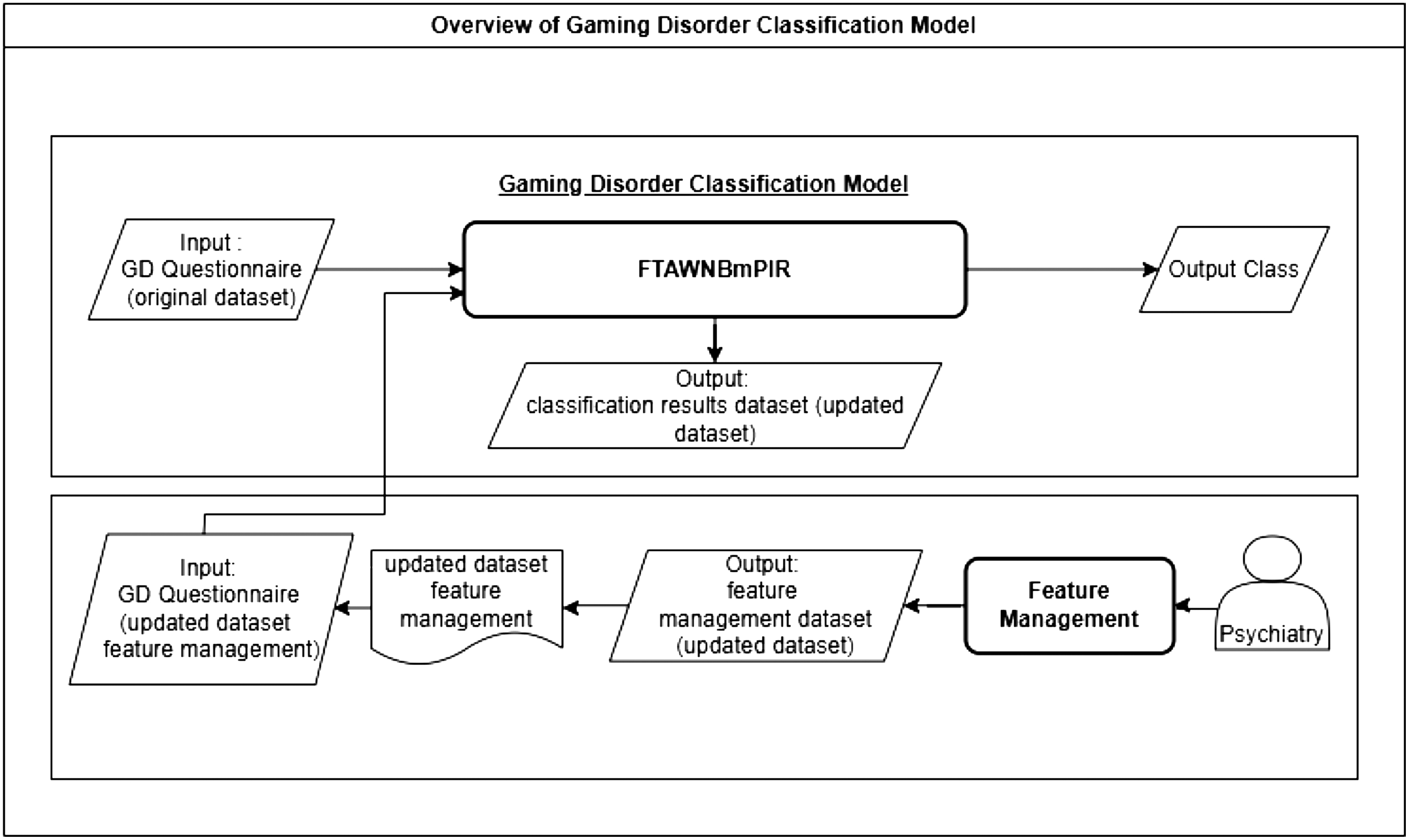Fig. 1. Overview of gaming disorder classification model.

An overview of the model development stages is illustrated in Fig. 2. The process begins with data collection, where the data used in this model come from questionnaires utilizing an early detection tool for GD. The data collection procedure has passed ethical feasibility testing and received research approval from the Medical and Health Research Ethics Committee, Faculty of Medicine, Public Health, and Nursing, Universitas Gadjah Mada, under ethical approval number KE/FK/0090/EC/2024. The data collection technique used in this research involved distributing an online questionnaire to participants. The questionnaire data, which served as training data, were gathered by distributing online forms to children aged 12 to 20 years. This method enabled efficient and convenient data collection, as respondents could complete the questionnaire remotely and at their own pace. Additionally, the online format facilitated broader outreach and ensured that the collected data were digitally organized, making it easier to analyze. The dataset contains 782 instances and 45 attributes. There are 44 attributes that are early signs of GD. These attributes have considered the criteria in DSM-V and ICD-11 that are suitable for early detection of GD, while the 45^th attribute is used as a class label. This study uses two classes, namely the GD class, to label data that is gaming disordered and the No class to label data that is not gaming disordered

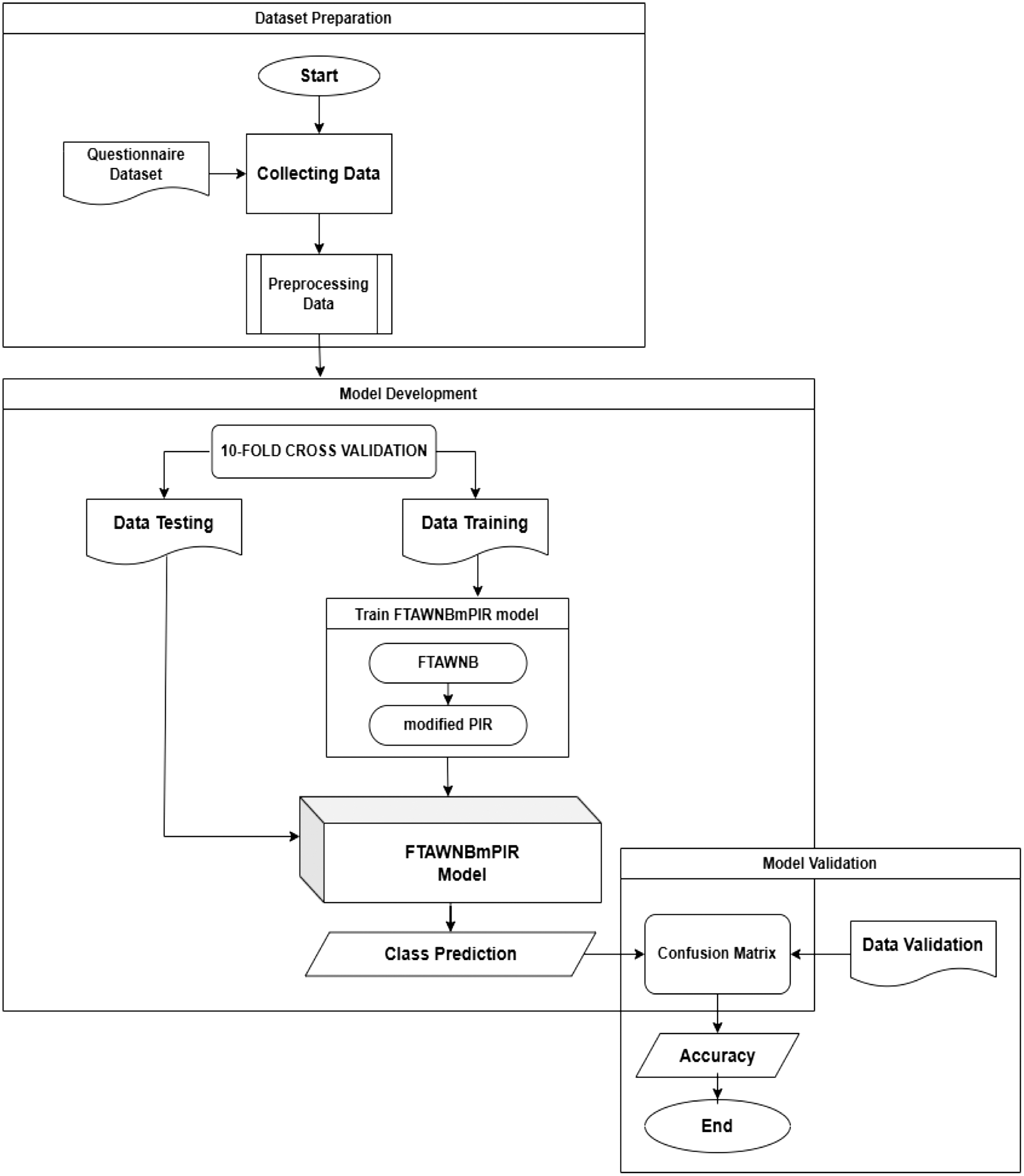Fig. 2. FTAWNBmPIR classification model development stages.

The next stage involves data preprocessing to process the available raw data. In this phase, the questionnaire data is analyzed to select the features to be used. The raw data are transformed into a clean and structured format, ready for the model evaluation process. Model evaluation is conducted using 10-fold cross-validation. The data are split into training and testing sets. These datasets are used to develop the FTAWNB with modified PIR model, which is a combination of the FTAWNB model and a modified PIR technique. Meanwhile, the validation data are used to validate the previously developed FTAWNB with modified PIR model to produce accurate class predictions. Validation is carried out using a confusion matrix to assess the classification accuracy by comparing the predicted classes with the actual classes.

A.INITIALIZING CONDITIONAL PROBABILITIES PHASE

The conditional probability is initialized in the first phase by utilizing correlation-based attribute weighting. Each attribute is given a continuous weight between 0 and 1 using attribute weighting. The exponential component of the conditional probability is then fed the weight of each attribute, w_j. Equation (7) represents the initialized conditional probability of FTAWNB. Equation (4) uses the weight of the j_th attribute, w_j, to determine the conditional probability of A_j = a_j given the class c, which is P(a_j|c).

P^{'} (a_{j} | c) = P {(a_{j} | c)}^{w j},

(7)

The attribute weights are assigned in the first phase by evaluating both the redundancy between attributes and their relevance to the classes. This process is referred to as initializing conditional probabilities. In this phase, conditional probabilities are used to establish and quantify the relationship between each pair of discrete random variables. Equations (8) and (9) outline the calculations for attribute-class relevance and the intercorrelation between attributes, respectively. Here, I(A_j;A_k) represents the intercorrelation between attributes, while I(A_j;C) represents the relevance of an attribute to a class. P(c) in equation (8) is the prior probability obtained based on equation (3).

I (A_{j}; C) = \sum_{a j} \sum_{c} P (a_{j}, c) l o g \frac{P (a_{j}, c)}{P (a_{j}) P (c)},

(8)

I (A_{j}; A_{k}) = \sum_{a j} \sum_{a k} P (a_{j}, a_{k}) l o g \frac{P (a_{j}, a_{k})}{P (a_{j}) P (a_{k})},

(9)

Normalization is applied to NI(A_j;C) and NI(A_j;A_k) using Equations (10) and (11) to ensure that I(A_j;C) and I(A_j;A_k) values are kept within the range of [0,1]. The symbol I(A_j; C) in equation (10) is the relevance of an attribute to a class obtained from equation (8).

N I (A_{j}; C) = \frac{I (A_{j}; C)}{\frac{1}{m} \sum_{j = 1}^{m} I (A_{j;} C)},

(10)

N I (A_{j}; A_{k}) = \frac{I (A_{j}; A_{k})}{\frac{1}{m (m - 1)} \sum_{j = 1}^{m} \sum_{k = 1 \land k \neq j}^{m} I (A_{j;} A_{k;})},

(11)

The weight of the j_th attribute, D_j, is then calculated using the subtraction approach as shown in Equation (12). Equation (12) shows how the attribute weight is calculated by proportionally decreasing the normalized mutual relevance and the normalized average mutual redundancy. Since D_j, as defined in Equation (12), can result in a negative value, it is adjusted to the range [0, 1] using the standard sigmoid logistic function in Equation (13), where w_j represents the discriminatory weight of the j_th attribute.

D_{j} = N I (A_{j}; C) - \frac{1}{m - 1} \sum_{k = 1 \land k \neq j}^{m} N I (A_{j}; A_{k})

(12)

w_{j} = \frac{1}{1 + e^{- D j}}

(13)

B.FINE-TUNING CONDITIONAL PROBABILITIES PHASE

The second stage involves fine-tuning based on the conditional probabilities of the training cases. For each training instance T_i (i = 1, 2, …, n), the class label (C_prediction) is predicted in sequence. If a training instance is misclassified (C_prediction ≠ C_actual), the corresponding conditional probabilities are adjusted. Equations (7) and (8) offer a detailed explanation of the fine-tuning process for each misclassified instance, where c_actu and c_pred represent the actual class and the predicted class, respectively.

P^{'} (a_{j} | c_{a c t u}) = P^{'} (a_{j} | c_{a c t u}) + δ (a_{j,} c_{a c t u})

(14)

P^{'} (a_{j} | c_{p r e d}) = P^{'} (a_{j} | c_{p r e d}) - δ (a_{j,} c_{p r e d})

(15)

Subsequently, the learning rate is regulated by the parameter η ∈ [0, 1]. Similarly, δ(a_j,c_pred) needs to be decreased in proportion to the error, which is the difference between β. P'(a_j|c_pred) and P’min(a_j|c_pred), as well as the learning rate η. Equations (16), (17), and (18) outline the formulas for adjusting the step sizes δ(a_j,c_actu) and δ(a_j,c_pred) according to this approach.

δ (a_{j}, c_{a c t u}) = η . (α . {P^{'}}_{m a x} (a_{j} | c_{a c t u}) - P^{′} (a_{j} | c_{a c t u})) . e r r o r

(16)

δ (a_{j}, c_{p r e d}) = η . (β . P^{′} (a_{j} | c_{p r e d}) - {P^{'}}_{m i n} (a_{j} | c_{p r e d})) . e r r o r

(17)

e r r o r = P (c_{p r e d} | T_{i}) - P (c_{a c t u} | T_{i})

(18)

C.MODIFIED PIR PHASE

The third phase starts by identifying outliers through the calculation of the Euclidean distance between each instance and the centroid of its actual class. An instance is classified as an outlier if its closest distance to a class centroid differs from the predicted class. Equation (19) is used to compute the center point c on the a_j attribute, where n represents the total number of instances in class c, i refers to the instances, and v_(i| $a_{j}$ ₎ is the value of row i for attribute n with label c. Meanwhile, Equation (20) calculates the distance between each data point and the cluster center, where d(i,c) represents the distance between data point i and the center of cluster c, x₍ $a_{j}$ _,i) is the i_th data point for attribute a_j, and x₍ $a_{j}$ _|c)is the center point of class c for attribute a_j.

x_{(a_{j} | c)} = \frac{1}{n} \times \sum_{i = 0}^{n} v_{(i | a_{j})}

(19)

d (i, c) = \sqrt{[{(x_{1, i} - x_{1, c})}^{2} + {(x_{2, i} - x_{2, c})}^{2} + \dots + {(x_{a_{j}, i} - x_{a_{j}, c})}^{2}]}

(20)

At this stage, the information gain (IG) value of each attribute is calculated and then ranked from smallest to largest. This study uses two classes: GD and NO (not GD). Let the set of examples T contain gd counts of class GD and no counts of class NO. The amount of information needed to decide if an arbitrary example in T belongs to GD or No is defined as Equation (21) below.

I (g d, n o) = - \frac{g d}{g d + n o} l o g_{2} \frac{g d}{g d + n o} - \frac{n o}{g d + n o} l o g_{2} \frac{n o}{g d + n o}

(21)

Assume that using attribute a_j, the set T will be partitioned into sets {T₁, T₂, …, T_n}. If T_i contains gd_i examples of GD and no_i examples of NO, the entropy, or the expected information needed to classify objects in all subtrees, is shown in Equation (22).

E (a_{j}) = \sum_{i = 1}^{n} \frac{g d_{i} + n o_{i}}{g d + n o} I (g d_{i}, n o_{i})

(22)

The information that would be obtained by branching on attribute a_j would then be calculated by Equation (23).

G a i n (a_{j}) = I (g d, n o) - E (a_{j})

(23)

These calculations are repeated for each and every attribute. Furthermore, instances identified as outliers are replaced with attribute values, starting from the attribute with the lowest IG value to the highest, based on the number of selected attributes. The modified PIR technique proposed in this study replaces outlier data values using a NB weighting approach, unlike the original PIR technique, which replaced missing values in outlier-class data. Attributes with the lowest information gain and those furthest from the class centroid are treated as outliers. The attribute values from the outlier data are replaced with the characteristics with the greatest probability values in the real class.

Figure 3 shows the stages of the FTAWNB with modified PIR (FTAWNBmPIR) model in feature management. This study tested this model with two testing schemes. Figure 3(a) depicts feature management from the first scheme utilizing the original GD dataset. The second approach, as shown in Fig. 3(b), takes advantage of the updated GD dataset generated during the third phase

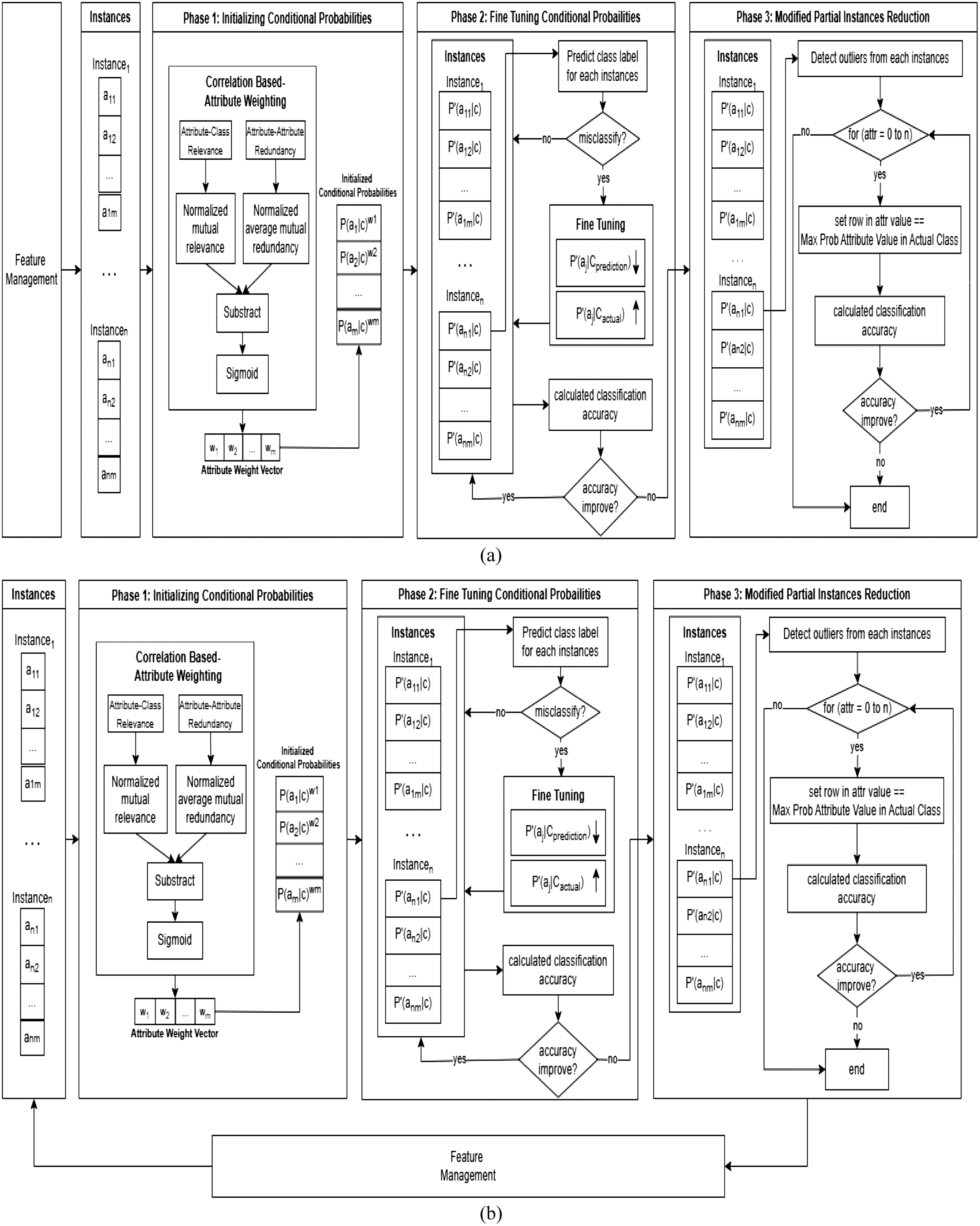Fig. 3. Framework FTAWNB with modified PIR Applied to Feature Management. (a) Proposed model using original GD dataset. (b) Proposed model using updated GD dataset.

IV.RESULT AND DISCUSSION

This study compares the performance of the FTAWNB and FTAWNBmPIR models in terms of feature management. The number of original features in the GD measuring instrument currently used is 44 features. Table I shows a comparison with two feature management scenarios, namely remove features and add features. In the feature elimination scenario, the four attributes with the lowest Information Gain values were removed from the dataset to reduce dimensionality and potentially enhance model performance. As a result, the number of features used in this scenario is reduced to 40 features. Meanwhile, for the add feature scenario, one new feature is added so that the number of features used in this scenario becomes 45 features.

Table I. Result of cross-validation using the original GD dataset

Parameter	FTAWNB (remove feature)	FTAWNBmPIR (remove feature)	FTAWNB (add feature)	FTAWNBmPIR (add feature)
Accuracy	98.47%	99.87%	98.59%	99.87%
Correctly Classified Instances	770	781	771	781
Incorrectly Classified Instances	12	1	11	1
Kappa statistic	0.945	0.9954	0.9494	0.9954
Mean absolute error	0.0192	0.004	0.0178	0.0034
Root mean squared error	0.0998	0.0404	0.0965	0.0395
Relative absolute error	6.9568%	1.4488%	6.457%	1.2252%
Total number of Outliers	79	6	70	16
Total number of instances	782	782	782	782

Table I shows the results of cross-validation using the original GD dataset. The accuracy obtained by the FTAWNB model in the remove feature scenario is 98.47%, while the FTAWNBmPIR model reaches 99.87%. In the add feature scenario, the FTAWNB model obtains an accuracy of 98.58%, and the FTAWNBmPIR model obtains an accuracy of 99.87%. The data misclassified by the FTAWNBmPIR model are less than that of the original FTAWNB model for the two tested feature management scenarios. The same thing happens; the amount of outlier data produced by the FTAWNBmPIR model is also less than the FTAWNB model. The number of outliers detected by the FTAWNBmPIR model in the feature remove scenario was 6 outlier data. There is a reduction in the number of outlier data by 70 data from the number of outliers detected by the FTAWNB model. A similar case was observed in the attribute addition scenario, in which the FTAWNB model identified 70 outliers, whereas the FTAWNBmPIR model identified only 16.

Table II shows the results of cross-validation using the updated GD dataset. The best performance in the feature remove scenario was obtained in the FTAWNBmPIR model with an accuracy of 99.87% compared to the FTAWNB model, which obtained an accuracy of 99.47%. Meanwhile, for the add feature scenario, these two models provide the same accuracy results. The number of outliers detected by the FTAWNBmPIR model for the feature remove scenario is less than the FTAWNB model. The FTAWNB model detected a total of 79 outliers, whereas the FTAWNBmPIR model detected only 6 outliers. In the feature addition scenario, the number of detected outliers remained unchanged, resulting in a consistent level of model accuracy. A total of 45 outliers were detected by both models.

Table II. Result of cross-validation using updated GD dataset

Parameter	FTAWNB (remove feature)	FTAWNBmPIR (remove feature)	FTAWNB (add feature)	FTAWNBmPIR (add feature)
Accuracy	99.47%	99.87%	99.74%	99.74%
Correctly Classified Instances	770	781	780	780
Incorrectly Classified Instances	12	1	2	2
Kappa statistic	0.945	0.9954	0.9908	0.9908
Mean absolute error	0.0192	0.004	0.0077	0.008
Root mean squared error	0.0998	0.0404	0.055	0.0541
Relative absolute error	6.97%	1.45%	2.7713%	2.883%
Total number of Outliers	79	6	45	45
Total number of instances	782	782	782	782

As shown in Table III, the performance of the model for feature management is evaluated by measuring the accuracy, precision, and recall values using two different datasets (the original GD dataset and the updated GD dataset). The FTAWNBmPIR model is able to provide the best performance by showing an increase or maintaining the accuracy, precision, and recall values. The FTAWNBmPIR model consistently outperforms FTAWNB across both the original and updated datasets. The updated dataset results in slightly better performance in both models, as seen from the higher accuracy, precision, and recall percentages. On the original dataset, adding features to the models generally leads to better performance compared to removing features, especially in the FTAWNBmPIR model.

Table III. Model performance comparison

Model	Feature management	Dataset	Accuracy	Precision	Recall
FTAWNB	Remove feature	GD original	98.47%	98.5%	98.5%
FTAWNBmPIR	Remove feature	GD original	99.87%	99.9%	99.9%
FTAWNB	Add Feature	GD original	98.59%	98.6%	98.6%
FTAWNBmPIR	Add Feature	GD original	99.87%	99.9%	99.9%
FTAWNB	Remove feature	GD Updated	98.47%	98.5%	98.5%
FTAWNBmPIR	Remove feature	GD Updated	99.87%	99.9%	99.9%
FTAWNB	Add Feature	GD Updated	99.74%	99.7%	99.7%
FTAWNBmPIR	Add Feature	GD Updated	99.74%	99.7%	99.7%

Figure 4 presents a comparative analysis of model performances across different scenarios involving feature management and dataset variations. This Figure illustrates the performance of two models, FTAWNB and FTAWNBmPIR, in terms of accuracy, precision, and recall. Each scenario compares the impact of feature addition and removal on both the original and updated GD datasets.

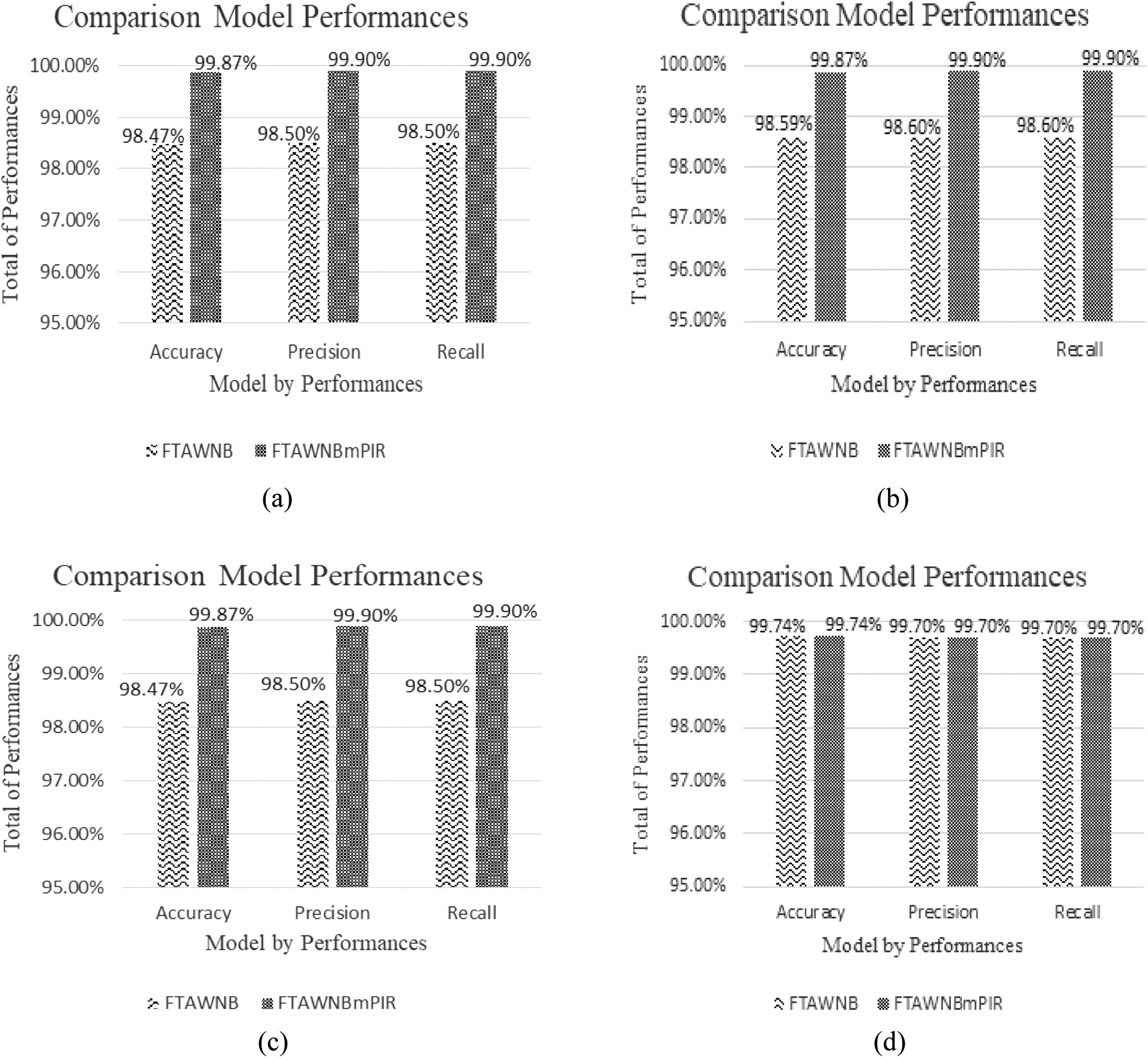Fig. 4. Comparison model performances to management features in GD dataset. (a) Model performance to feature removal scenario on original GD dataset. (b) Model performance to feature addition scenario on original GD dataset. (c) Model performance to feature removal scenario on updated GD dataset. (d) Model performance to feature addition scenario on updated GD dataset.

FTAWNBmPIR outperforms FTAWNB on all metrics in Fig. 4(a), showing a significant gain in accuracy, precision, and recall following the removal of features from the original GD dataset. Figure 4(b) shows that both models perform better when features are added to the original dataset. FTAWNBmPIR performs better, reaching nearly 99.9% in precision and recall.

Figure 4(c) shifts focus to the updated GD dataset under a feature removal scenario. Here, FTAWNBmPIR maintains its higher performance, demonstrating consistent accuracy (99.87%) and enhanced precision and recall over FTAWNB. It is also shown in Fig. 4(d) that both models perform optimally in this scenario, with the same accuracy gain of 99.74%. These results suggest that both feature addition and the use of an updated dataset contribute positively to model performance, with FTAWNBmPIR consistently outperforming FTAWNB.

In Scenario 1, which involved the addition of one attribute, the baseline FTAWNB model demonstrated solid classification performance on the original dataset. However, after integrating the mPIR technique, the model’s accuracy improved by 1.28%. This improvement suggests that the modified PIR technique enhances the instance selection process by effectively filtering out less relevant data points. As a result, the model achieves better generalization, even with minimal changes in the feature space, indicating improved robustness to incremental feature additions.

When tested on the updated dataset, the FTAWNB model with modified PIR maintained an exceptionally high accuracy of 99.74%, showing no significant decline in performance despite the addition of a new attribute. This result highlights the model’s resilience in adapting to newly introduced features. The stable performance reflects the model’s capacity to handle dynamic changes in the input structure, reinforcing its applicability in real-world environments where mental health indicators may evolve over time.

In Scenario 2, which involved the removal of four attributes, the performance of the baseline FTAWNB model experienced a slight decline when applied to the original dataset. However, after applying the modified PIR technique, the model’s accuracy improved by 1.4% compared to its baseline performance under the same conditions. The improvement indicates that the modified PIR technique is capable of compensating for reduced feature availability by selecting the most informative instances. This suggests that even when the input data loses important attributes, the model maintains reliable classification performance by focusing on data quality over quantity.

On the updated dataset, the FTAWNB with modified PIR model also achieved an accuracy improvement of 1.4%, maintaining consistent performance despite the intentional reduction in input attributes. This consistency further supports the effectiveness of the modified PIR in enhancing model adaptability. The ability to preserve high accuracy when faced with incomplete or reduced feature sets confirms that the model is well-suited for dynamic and imperfect data conditions commonly found in real-world mental health applications.

A.RESEARCH CONTRIBUTIONS AND FINDINGS

This study contributes to the advancement of mental health classification by developing a novel model—FTAWNB integrated with a mPIR technique—that is designed to maintain robustness despite dynamic changes in dataset attributes. The model specifically addresses challenges arising from evolving symptom patterns in GD by testing its performance under scenarios involving the addition and removal of attributes, thereby simulating real-world variability in data. Through the integration of the modified PIR technique, the model demonstrates enhanced stability and improved classification accuracy compared to baseline approaches.

The key findings from this research reveal that the proposed FTAWNB with modified PIR model improved classification accuracy by 1.28% and 1.4% in scenarios of attribute addition and removal on the original dataset. Furthermore, on the updated dataset, the model maintained a high accuracy of 99.74% during attribute addition and further improved accuracy by 1.4% during attribute removal. These results highlight the model’s robustness in handling dynamic and changing feature sets, which is critical for reliable classification in evolving social environments.

Overall, the findings support the potential application of this model as a dependable tool for early detection and classification of GD, a condition recognized in ICD-11 by the World Health Organization. The model’s consistent performance across both original and updated datasets indicates its suitability for practical implementation in real-world mental health screening and diagnostic systems, particularly in contexts where symptomatology and diagnostic criteria may change over time.

V.CONCLUSION AND FUTURE WORK

This study successfully addressed the challenges associated with dynamic symptomatology and evolving data attributes in the classification of GD by proposing a FTAWNB model, integrated with a mPIR technique. The model was evaluated under two practical scenarios involving feature addition and removal. Empirical results indicated consistent improvements in classification performance, with accuracy increases of 1.28% and 1.4% on the original dataset for the respective scenarios. Notably, the model maintained a high accuracy of 99.74% on the updated dataset in the addition scenario and demonstrated further improvement under the removal condition. These outcomes affirm the model’s robustness and adaptability in handling fluctuating feature sets, which are essential for reliable mental health diagnostics in dynamic environments. The proposed approach demonstrates significant potential as a reliable tool for early detection and classification of GD in both clinical and community-based contexts. Future work may explore its generalizability to other mental health conditions characterized by similarly variable features.

Robust Feature Management for Gaming Disorder Classification Using Modified Partial Instance Reduction and Fine-Tune Attribute-Weighted Naïve Bayes