I.INTRODUCTION
Software consists of instructions written in a programming language that allow a computer to carry out specific tasks [1]. A software defect refers to an error or flaw in the code that causes the software to behave unexpectedly or incorrectly [2]. Software defect prediction (SDP) is an area in software engineering aimed at identifying fault-prone components in a software system before they lead to failures [3]. Predicting software defects helps in prioritizing testing and maintenance efforts, ultimately improving software reliability and reducing cost and time [4]. Programming involves constructing software through code, which may contain errors due to logical flaws or miscommunication [5]. Traditional defect prediction techniques have relied heavily on statistical and machine learning techniques using handcrafted features extracted from software metrics [6]. As software systems have become more complex and dynamic, traditional approaches are struggling to capture the temporal and relational dependencies in data, leading to reduced effectiveness [7]. Recently, deep learning (DL) models have shown promise in handling such complexities by learning useful features from raw data automatically, mostly in time series and sequential data structures [8]. Techniques like Bidirectional Long Short-Term Memory (BiLSTM) networks and attention-enabled models are increasingly used for capturing sequential dependencies and enhancing defect prediction accuracy [9]. The use of temporal collaborative attention mechanisms helps in forecasting and identifying hidden defect patterns in evolving software effectively [10]. The clustering techniques and unsupervised learning approaches are being explored for effort-aware defect prediction, where labeled data may be scarce [11]. Hybrid models combining oversampling methods and neural architectures have proven effective in addressing imbalanced data issues [12]. These advanced methods often utilize sensor signal data, shared temporal attention layers, and transformer-based encoders to reveal deeper insights about code reliability and degradation over time [13]. Researchers emphasize the need for explainable prediction models in SDP to help developers to understand the reasoning behind defect forecasts [14]. SDP is evolving with modern AI techniques, enabling proactive quality management and reducing maintenance costs [15]. Integrating domain knowledge with machine learning improves prediction relevance and supports better decision-making during development [16].
Existing SDP approaches face several challenges. Many struggles are faced to effectively capture both temporal and relational dependencies in dynamic software systems, leading to reduced prediction accuracy. The interconnected nature of modern codebases makes it difficult to model how changes in one module impact others, while optimizing model parameters remains computationally intensive.
The motivation behind this work stems from the limitations observed in existing SDP techniques, which often fail to effectively handle the temporal evolution of code and the relational dependencies between software modules. As software systems become more complex and interconnected, there is a growing need for models that can accurately capture both time-dependent behaviors and structural relationships. This work is motivated by the goal of developing a more robust, scalable, and accurate prediction model through Temporal Transformer Graph Convolutional Network with Newton–Raphson Optimization (TTRGCN-NRO), thereby improving early defect detection, reducing software maintenance costs, and enhancing overall software quality.
The main contributions of the research on SDP are as follows:
- •The objective of this work is to enhance the accuracy of SDP and support effective risk management. It aims to address common challenges in defect datasets, such as data imbalance, noise, and high dimensionality. This work focuses on improving predictive reliability and overall software quality assessment. The novelty of this approach lies in the use of the TTRGCN-NRO method, which leverages advanced graph convolutional techniques combined with noise reduction and optimization strategies to achieve superior performance in defect prediction.
- •The preprocessing stage focuses on improving data quality before model training. It involves normalizing the data, removing outliers, and balancing class distributions to address common issues like noise and imbalance. These steps ensure cleaner, more representative datasets that enhance prediction performance.
- •In feature selection, the process focuses on reducing irrelevant or redundant features to simplify the dataset. It uses an iterative approach combined with validation to identify and keep the most important features. It results in improved model efficiency, accuracy, and generalization.
- •For prediction, the proposed model captures complex spatial and temporal relationships within the data to improve prediction accuracy. NRO is the optimization technique that enhances learning efficiency and convergence speed, resulting in more reliable predictions. The proposed TTRGCN-NRO method has achieved an accuracy of 1.00 on the CM1 dataset and a precision of 0.93 on KC2. It has recorded 0.82 for recall on JM1 and 0.98 for F1-score on PC1, demonstrating strong and consistent defect prediction performance.
The following sections of the research are formatted as follows: In Section II, the essential research is reviewed. The research methodology is explained in Section III, results and discussions are described in Section IV, and the conclusion is reviewed in Section V.
II.LITERATURE REVIEW
Previous works on SDP are mentioned below.
In 2024, [17] investigated the Graph Attention Transformer (GA-Tran) model, which enhances transformer networks for fault detection by combining spatial-temporal learning and addressing process variable coupling. In 2023, [18] introduced the Graph Attention Transformer-Deep Adaptive Transformer (GAT-DAT) framework, which combines a deep adaptive transformer and graph attention network to improve spatial correlation extraction.
In 2024, [19] analyzed the new anomaly detection system that combines fast sequence modeling, graph learning, and a transformer model trained through two-stage adversarial training. In 2024, [20] introduced dynamic graphs and multi-level features. The Spatial-Temporal Transformer with Double Recurrent Graph Convolutional Network (STTDGRU) model improved traffic flow forecasting.
In 2024, [21] introduced the Spatio-Temporal Multi-Graph Transformer (ST-MGT), which enhances multi-vessel prediction and maritime safety. In 2023, [22] investigated the Transformer Enhanced-Temporal Convolution Network (TE-TCN) to capture temporal and spatial dependencies to increase the accuracy of prediction. In 2024, [23] introduced the Long-Short Term Spatiotemporal Neural Network (LSTSNN) to improve the SDP. Table I represents the comparison of SDP.
Table I. Recent works comparison
| Authors | Focus | Technique | Advantages | Limitations |
|---|---|---|---|---|
| [ | Finding flaws in complex procedures | GA-Tran | Effective defect finding for intricate processes | Large datasets needed for training; computational complexity |
| [ | Remaining a useful life forecast | Graph GAT-DAT | Enhanced RUL forecast precision | Possible overfitting |
| [ | Identifying and categorizing anomalies in multivariate time series | GA-Tran | Improved multivariate anomaly detection | May have trouble with unstructured or extremely noisy data |
| [ | Predicting traffic flow in spatiotemporal contexts | STTDGRU | Predicting the flow of traffic with accuracy and spatial-temporal connections | High processing demands for predictions |
| [ | Predicting the course of a vessel | ST-MGT | Accurate joint prediction of various vessel trajectories | Managing sparse data from different vessels might be challenging |
| [ | Forecasting traffic flow | TE-TCN | Increased accuracy in predicting long-term traffic flow | Could be affected by the hyperparameter selection |
| [ | Forecasting traffic flow | LSTSNN | Efficient representation dependency in traffic data | Need a significant amount of historical data with labels |
A.PROBLEM STATEMENT
Previous research on SDP faces notable limitations. The approach in [17] discusses the issue of high computational complexity, while the model proposed in [18] is prone to overfitting in complex scenarios. It reports difficulties in accurately detecting anomalies when the data is noisy or unstructured [19]. Traffic prediction models are hindered by high processing demands [20], sensitivity to hyperparameter tuning [22], and reliance on large labeled datasets [23]. Vessel trajectory forecasting also faces challenges in handling sparse, diverse data sources [21]. These issues highlight the need for models that balance accuracy with efficiency and robustness across diverse data conditions. In order to overcome these issues, “Software Defect Prediction in Risk Management Using Temporal Transformer Graph Network with Newton-Raphson Optimization” is developed for precise analysis and useful evaluation.
III.PROPOSED METHODOLOGY
The proposed workflow is shown in Fig. 1. The SDP process begins with data preprocessing using Quantile Transformer (QT), Local Outlier Factor (LOF), and GLOW Synthetic Minority Oversampling Technique (GLOW SMOTE)-Density. The Recursive Feature Elimination with Cross-Validation (RFECV) is used to reduce the feature dimensions. Finally, TTRGCN-NRO ensures proper performance when used in risk management for SDP. By increasing overall risk management and prediction accuracy, it offers a better solution.
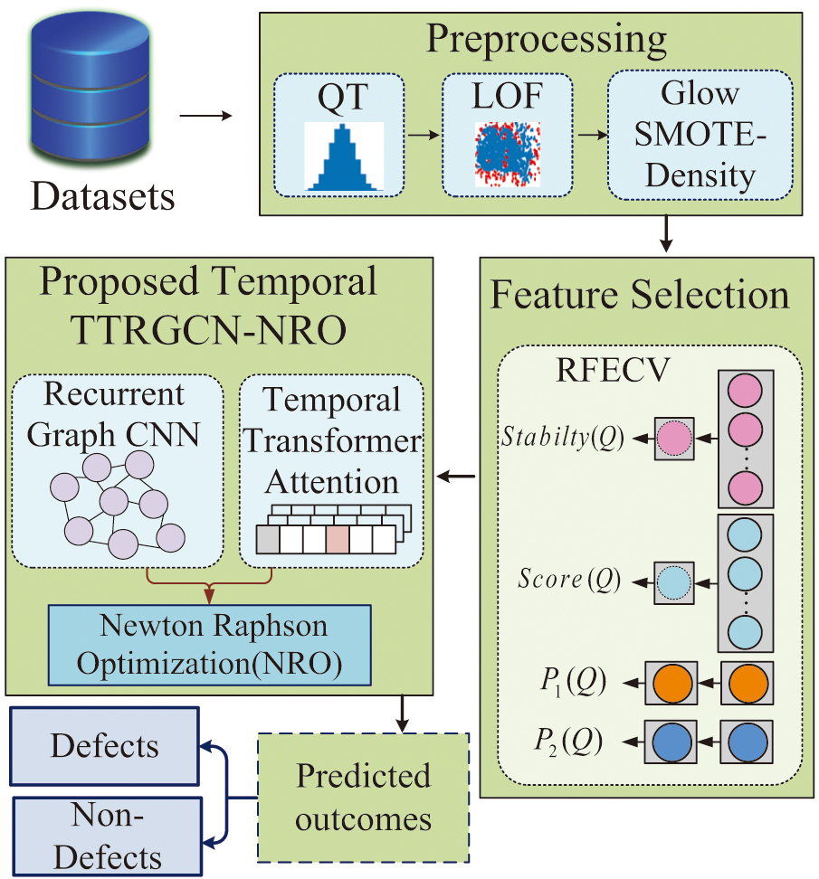 Fig. 1. Schematic view of the overall proposed methodology.
A.DATA COLLECTION
The input data for SDP is gathered from the CM1 [24], JM1 [25], KC1 [26], KC2 [27], and PC1 [28] datasets. The collected data is subjected to preprocessing.
B.PREPROCESSING
In SDP, preprocessing involves balancing the dataset, managing outliers, and normalizing data to enhance model performance.
1).QT FOR NORMALIZATION
For improved expression and sequential interrelation capture, the QT model combines Long Short-Term Memory (LSTM), Multi-Head Attention (MHA), and dense layers. and the Adam optimizer are used for effective data processing and forecasting. Also, with the encoder output serving as a query in the transformer, the QT model manages and forecasts data by combining LSTM layers, MHA, and dense layers. To increase forecasting accuracy, the model applies dropout, normalizes input data, and reshapes the query tensor. By combining several layers and transformations, this design improves generalization and performance after the data is normalized [29].
2).LOF FOR DATA CLEANING
LOF [30] is an unsupervised method that detects outliers by comparing a point’s local density with its neighbors using reachability distance (RD) and local reachability density (LRD). It outperforms traditional methods by adapting to local patterns, handling noise, and spotting subtle anomalies. LOF is ideal for identifying unusual behavior in complex datasets. LOF is involved in data cleaning by removing missing values and duplicates and normalizing data before applying LOF to detect and eliminate outliers for better data quality. RD is calculated by using k-distance and the maximum distance between two points. Equation (1) shows the RD between two points:
where denotes the RD from instance and , denotes the actual distance between point and , and represents the distance from the point to its k-th nearest neighbor (KNN). RD is the k-distance of an object and is used to calculate the LRD, which is based on the RD to its KNNs, as shown in Equation (2):where denotes the point , denotes the set of KNNs of , denotes the RD between two points as and individual neighbor, and denotes the number of neighbors. LOF is calculated by comparing LRD ratios of a point’s k-neighbors, with higher LOF indicating outliers, as mentioned in Equation (3):LOF identifies outliers by analyzing deviations from usual patterns, such as unusual user actions in insider software prediction. Higher LOF values indicate stronger outliers in the dataset.
3).GLOW SMOTE-DENSITY FOR DATASET BALANCING
GLOW SMOTE-Density [31] improves dataset balance by generating synthetic samples based on minority class density patterns. To generate synthetic samples, the method first defines a distance function to measure similarity between two samples based on their feature values and corresponding weights. The global distance function can be represented in Equation (4).
where denotes the total distance between and , which is calculated as the weighted sum of individual feature distance as , is total features, and is weight of features . The performance of can be calculated using the Value Difference Metric in Equation (5):where denotes the number of class labels. The first time initialized with 1 and two discrete values are considered as a similar decision distribution. SMOTE generates synthetic samples, normalizing global weights. is mentioned in Equation (6).GLOW SMOTE-Density generates synthetic samples in high-density minority areas to balance datasets and improve model generalization. After preprocessing, the processed data undergoes RFECV to select the most relevant features, thereby optimizing model efficiency and predictive power.
C.RECURSIVE FEATURE ELIMINATION WITH CROSS-VALIDATION FOR FEATURE SELECTION
RFECV [32] is the feature selection technique that recursively removes the least important features based on model performance. It integrates cross-validation to prevent overfitting and improve robustness, making it more reliable than traditional filter or wrapper methods. RFECV is preferred due to its ability to balance accuracy, generalization, and feature relevance, particularly in high-dimensional datasets. Assuming that the RFECV-initialized feature set is chosen, the feature subset , or . The feature subset score is given in Equation (7).
where represents the cross-validation technique, denotes the score through the use of random sampling, and and represent the regularization term’s score.Score: To assess the generalization ability, the k-fold cross-validation is employed. The dataset is split into k parts, and in each iteration, one fold is utilized for validation set, while the remaining k − 1 folds are used for training. This process is repeated k times. The average score over models and k-folds is computed in Equation (8):
where represents the average analysis metric value for the feature subset obtained from the regression method under -fold cross-validation, denotes the number of models that get considered, and represents the expected evaluation metric validation set.Stability: The stability of the selected features is evaluated using a random sampling approach. The procedure includes choosing a portion of the data randomly to form testing and training sets, training models on this data and computing performance metrics, evaluating the average difference between predicted and actual labels, and repeating the above steps for n iterations. The final stability score is the average of the evaluation metrics over all repetitions and can be computed in Equation (9):
where denotes the score of stability for the extracted features, denotes the number of samples, and represents the evaluation metrics values that were evaluated in cross-validation and training.P1 and P2: Since regularization improves generalization and lowers complexity, improving predictive performance, regularization filters irrelevant features as mentioned in Equations (10) and (11).
where denotes the extracted features that regulate the term rating and represents the weight coefficient obtained upon regularization from the roles .where denotes the regularization term score related to the feature subset and denotes the weight coefficient obtained after regularization of the features . By combining the strengths of cross-validation, stability selection, and regularization, the RFECV algorithm offers a flexible and robust feature selection mechanism. With an optimized set of features, the next phase involves deploying a sophisticated DL model capable of capturing complex spatial and temporal dependencies within software defect data.D.PROPOSED TTRGCN WITH NRO
TTRGCN-NRO is a hybrid DL model that combines TTA, GRU, GCN, and NRO to capture both spatial and temporal dependencies in software defect data. It is chosen over existing models due to its ability to dynamically learn graph structures and long-range temporal relationships. Unlike traditional approaches, it effectively handles non-static code relationships and sequential behavior in evolving software. Compared to conventional models, it addresses limitations like static code analysis and weak temporal modeling. For SDP, it overcomes key challenges such as evolving software dependencies, imbalanced data, and multi-step forecasting. NRO further enhances convergence speed and solution quality, improving reliability in defect prediction. This makes TTRGCN-NRO highly effective for complex, real-world SDP tasks.
1).TTRGCN FOR SDP
The TTRGCN [33] model includes a GCN layer, GRU, TTA layer, and a convolutional layer. It is chosen for its ability to effectively capture both temporal and spatial dynamics in sequential data, making it suited for SDP tasks. Its integration of GCN and GRU allows for modeling complex spatial dependencies and local temporal patterns, while the TTA layer enhances long-range temporal relationships. This combination enables more accurate and adaptive representation learning in dynamic systems. To record fine-grained spatial correlations, the proposed model makes use of a spatial domain graph convolutional neural network, as stated in Equation (12):
where is a matrix of the graph’s neighbors, denotes the nonlinear activation role, represents the matrix of degrees of , and denotes the signal matrix. To save computational resources, is calculated as Equation (13):where denotes nonlinear activation functions, represents the graph convolution operation, and denotes the automatic updating continuously all through training. The graph convolution operation is then expressed in Equation (14):The proposed TTRGCN separates its predefined and dynamic adjacency matrices into distinct graph convolution operations. There is no predefined adjacency matrix used when . Instead, the GCN model uses a gate mechanism that enables it to eliminate irrelevant data from the predetermined adjacency matrix mentioned in Equations (15), (16), and (17):
where is the distance range with threshold among nodes , denotes the distance between , and represents the learnable variables. Features from adjacent nodes are combined into the central node by the GCN operation. Expressing parameters prevents all nodes from learning the same patterns. A node’s specific weight and partiality are denoted by and , as mentioned in Equations (18) and (19):The GRU operation effectively captures both spatial and temporal correlations, enhancing prediction accuracy in dynamic environments. The self-attention module of the TTA layer is shown in Fig. 2.
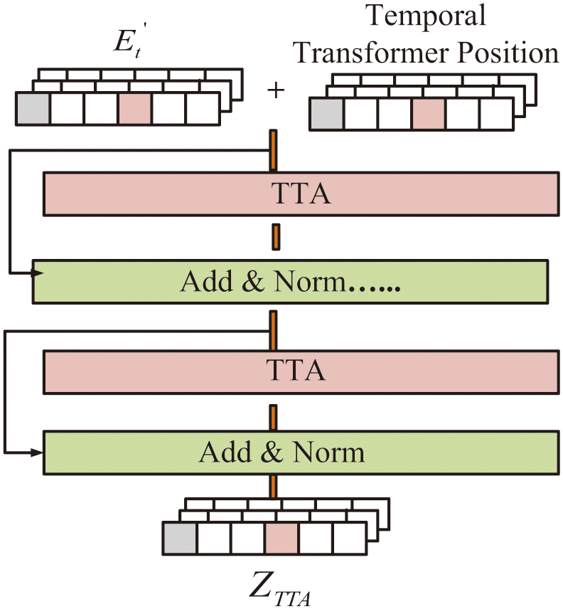 Fig. 2. The structure of the TTA layer.
A self-attention module with 1D convolution captures global nonlinear temporal correlations after the GRU layer. The attention score can be defined as mentioned in Equations (20) and (21):
where denotes a query, key, and value of their dimensions; denotes the convolution operation and linear transformation; denotes a key vector and the query convolution operation; represents the vector values that are linearly transformed; and indicates the feature dimension. Each position is treated equally by the self-attention mechanism models, which disregard sequential dependencies. Moreover, because of the stronger correlations between adjacent data points, the order information is crucial for modeling time-series data. To determine the location of in the sequence , the position code is used for a time slice as described in Equations (22) and (23). Equation (24) represents the TTA layer:where denotes the rectified unit operations like and , and represents the features. The prediction layer, which utilizes the 1D convolutional module, increases the accuracy of multi-step forecasting. It simultaneously predicts values and minimizes error accumulation. The model integrates GCN for spatial correlations, GRU for spatial-temporal dependencies, and TTA for global temporal patterns. The 1D convolutional layer enhances multi-step prediction by reducing error accumulation. The SDP output is passed to the NRO technique to improve training efficiency and model convergence.2).NRO TO IMPROVE THE CONVERGENCE SPEED
NRO [34] is a population-based metaheuristic algorithm that is employed to minimize the prediction error by guiding the model toward better weight configurations using its second-order search strategy. Unlike conventional gradient-based methods, NRO enhances the convergence speed and avoids local minima by combining Newton-inspired directional updates with adaptive control mechanisms. During training, it iteratively refines the parameters of the GCN, GRU, and TTA layers by evaluating candidate solutions based on the model loss function. It outperforms conventional metaheuristics by balancing diversification and intensification through adaptive parameters and Newton-inspired directional updates, which improves its capability to avoid local optima.
Initialization
Equation (25) defines the population matrix along with its overall dimensions.
where denotes the full population.Fitness function
To improve the convergence speed, NRO uses a differentiable error-based fitness function in Equation (26):
where denotes the output from the SDP and denotes the expected output from the NRO after the optimization process.Newton–Raphson Search Rule (NRSR)
By raising exploration susceptibility, the NRSR improves exploration accuracy and convergence speed. The differential perturbation step is calculated as in Equation (27):
where denotes the optimal solution, denotes the current individual, and denotes the random variables with options. The main position update rule inspired by Newton’s method is in Equation (28):where denotes the worst position in the neighborhood, denotes the best position among neighboring vectors, denotes the current individual position, and denotes the standard normal random number. The adaptive control parameter can be represented in Equation (29):where denotes the present iteration and denotes the greatest number of iterations. The parameter adjusts across iterations to maintain the equilibrium between exploration and exploitation. With this control, NRBO updates candidate positions using a blend of Newton steps and differential moves. The next-generation population is computed in Equations (30) and (31):where denotes the random number between . Despite the use of directional search, local minima traps may still occur. NRB addresses this issue using a trap-avoidance strategy.Trap-avoidance operator (TAO)
When NRBO detects stagnation or premature convergence (based on a diversification factor), it generates an alternative solution as in Equation (32):
where denotes the new position of the n-th individual at iteration. The parameters used by TAO are represented in Equations (33) and (34):where denotes the binary numbers, as either 1 or 0, and denotes the random numbers. The NRO promotes a balance between exploration and exploitation by optimizing the best fitness function. It enhances convergence speed and solution quality by combining adaptive parameters with the TAO operator.Termination
If the termination criteria are satisfied, the best solution is returned. Table II shows the pseudocode of a proposed methodology.
Table II. Algorithm of overall proposed methodology
| load_datasets load_datasets (‘CM1’, ‘JM1’, ‘KC1’, ‘KC2’,’ PC1’) |
| data = normalize_QT(data) |
| data = remove outliers_LOF(data) |
| data = balancing dataset_GLOW SMOTE Density(data) |
| features = RFECV_select_features(data) |
| features = RFECV_select_features(data) |
| model = TTRGCN_NRO( |
| input_dim=features.shape[1], |
| output_dim=1, |
| layers |
| { |
| 'TTA': True, |
| 'GRU': True, |
| 'GCN': True, |
| 'Conv1D': True |
| } |
| optimizer='NRO') |
| for epoch in range(epochs): |
| preds = model_forward(data[features]) |
| loss = calculate_loss(preds, labels) |
| while not terminated: |
| if stop_condition_met(): |
The proposed TTRGCN-NRO method is used for accurate SDP, effectively capturing both spatial and temporal patterns in software metrics. It uses dynamic and predefined adjacency matrices to model relationships between software components. NRO improves model convergence by applying adaptive Newton-based updates and a trap-avoidance strategy. Together, these components boost prediction accuracy, efficiency, and robustness.
IV.RESULTS AND DISCUSSIONS
SDP using the proposed TTRGCN-NRO model has demonstrated to be highly effective. The model is rigorously evaluated across multiple benchmark datasets for performance validation. Comprehensive analysis using precision, F1-score, Area Under the Curve (AUC) accuracy, and recall is conducted. Each dataset demonstrates superior results for the proposed method compared to existing techniques. Table III shows the system configuration used for training and evaluation of the SDP.
Table III. System configurations
| Components | Specifications |
|---|---|
| Operating system | Windows 10 |
| Python version | Python 3.12.7 |
| Processor | 2.15 GHz |
| RAM | 128 GB |
| Development environment | Visual Studio Code |
| Training iterations | 100 |
A.DATASET DESCRIPTION
Datasets CM1, JM1, KC1, KC2, and PC1 are used to evaluate the TTRGCN-NRO technique evaluation. This research focuses on software defect risk management using five datasets selected from the PROMISE Software Engineering Repository, which is publicly available and maintained by NASA’s Metrics Data Program. Predictive models commonly use these datasets to improve their performance.
1).EXPLORATORY DATA ANALYSIS
Figure 3 shows an exploratory analysis of the defect counts in five software defect datasets. In (a), the CM1 dataset contains 449 defective instances labeled as false and 49 non-defective instances labeled as true. In (b), the JM1 dataset includes 2,106 defective instances labeled as false and 8,779 non-defective instances labeled as true. In (c), the KC1 dataset has 326 defective instances labeled as yes and 1,783 non-defective instances labeled as no. In (d), the KC2 dataset has 105 defective instances labeled as yes and 415 non-defective instances labeled as no. In (e), the PC1 dataset consists of 77 defective instances labeled as false and 1,032 non-defective instances labeled as true. This figure highlights the class distribution in each dataset, which is often imbalanced between defective and non-defective instances.
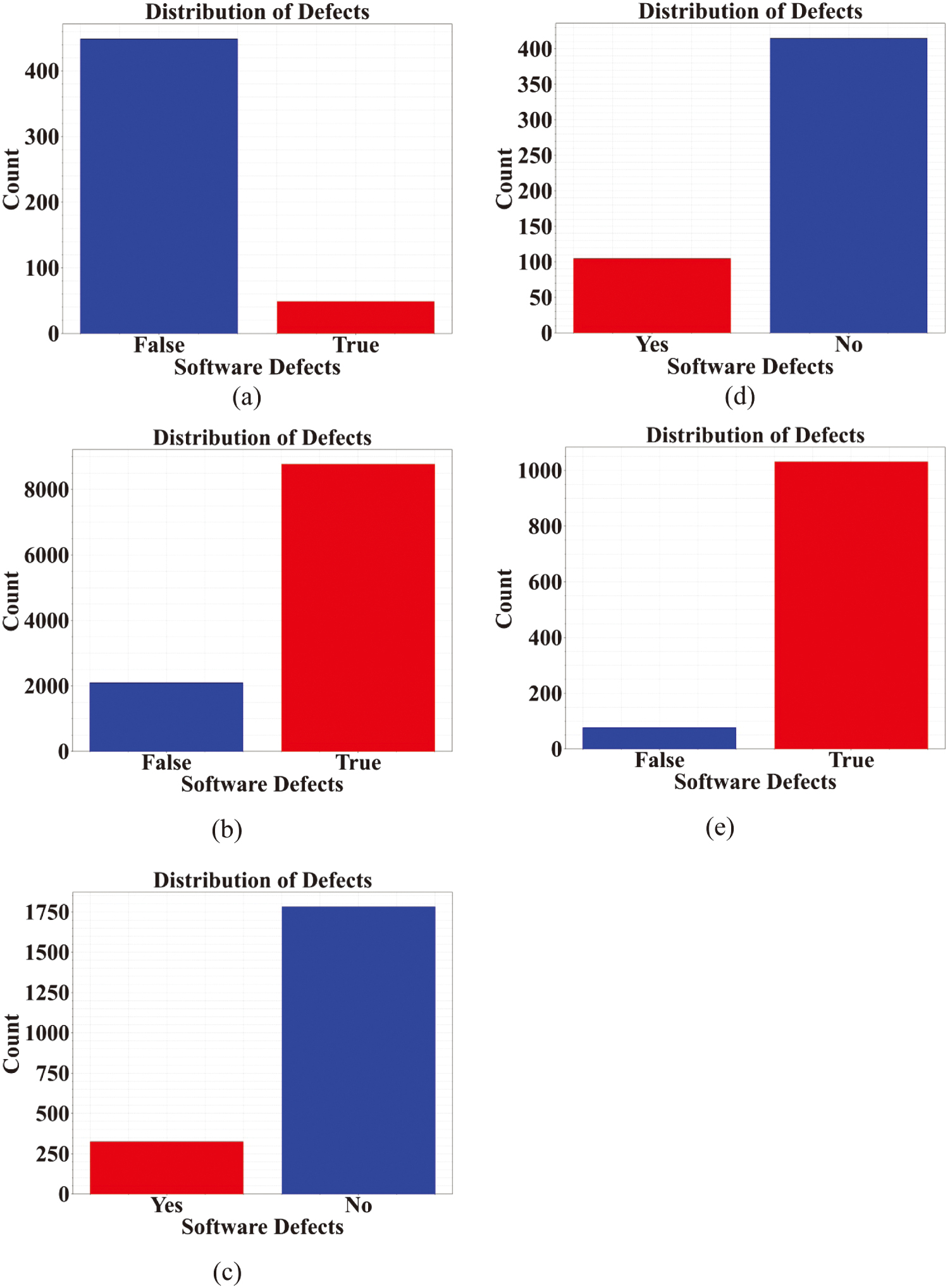 Fig. 3. Exploratory analysis of the defects count in the datasets a) CM1, b) JM1, c) KC1, d) KC2, and e) PC1.
B.LOF ANALYSIS
Figure 4 shows the LOF values before and after the data cleaning process. In (a), the LOF values indicate the presence of both outliers and inliers in the dataset, highlighting points that significantly deviate from their local neighborhoods. In (b), after the data cleaning process, the LOF values reflect the removal of outliers, retaining only the inliers.
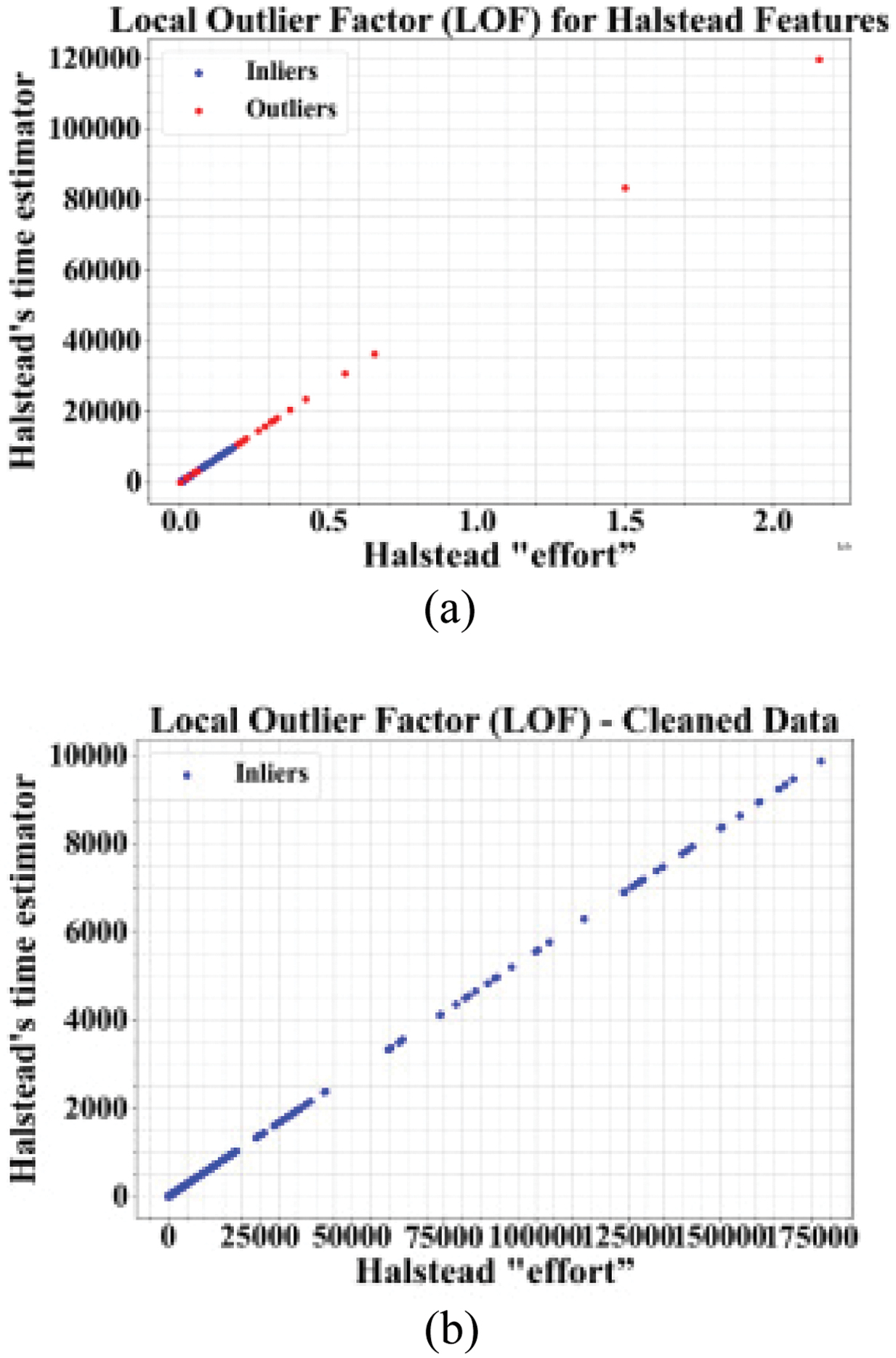 Fig. 4. LOF values (a) before and (b) after cleaning the data.
1).AVERAGE ACCURACY BEFORE AND AFTER OVERSAMPLING
Figure 5 shows the dataset imbalance issue and its solution using the GLOW-SMOTE density oversampling. Before oversampling, SMOTE-N for dataset balancing results in low accuracy, whereas the application of the GLOW-SMOTE density after the oversampling technique significantly improves prediction model accuracy, showcasing the importance of proper methods.
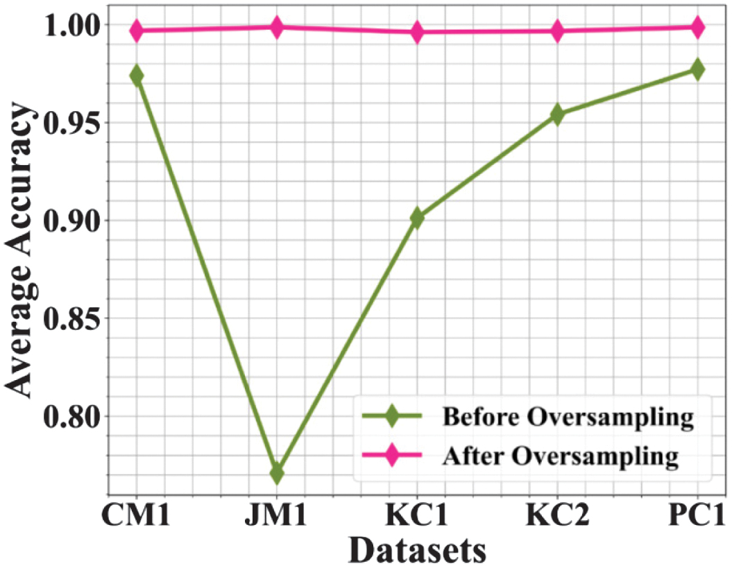 Fig. 5. Average accuracy before and after solving the class imbalance issue.
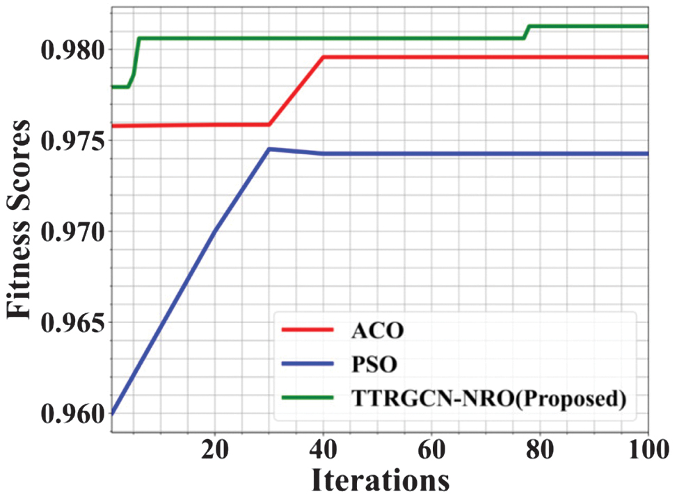
C.CONVERGENCE CURVE
Figure 6 shows the convergence performance of the proposed TTRGCN-NRO algorithm against Particle Swarm Optimization (PSO) and Ant Colony Optimization (ACO). The existing methods, such as PSO and ACO, reach a fitness score of 0.978 by the 40th iteration, and PSO attains 0.975 at the 30th iteration. The TTRGCN-NRO has achieved its optimal fitness value of 0.982 within just 10 iterations, showing its rapid convergence capability. The early convergence significantly reduces computational time, making it more efficient for real-time applications. Overall, TTRGCN-NRO demonstrates superior performance in both accuracy and speed over traditional optimization methods.
D.DEFECTS PREDICTION PERFORMANCE IN VARIOUS DATASETS USING TTRGCN-NRO
Figure 7 presents the performance analysis of three defect prediction methods, namely With Feature Selection (WFS), Without Feature Selection (WOFS), and the proposed method TTRGCN-NRO. The evaluation was carried out across five benchmark datasets, which include CM1, JM1, KC1, KC2, and PC1. In (a), the TTRGCN-NRO method has achieved an accuracy of 1.00 on the CM1 dataset, 0.78 on JM1, 0.90 on KC1, 0.89 on KC2, and 1.00 on PC1. When compared to the existing methods WFS and WOFS, the proposed method has recorded the highest accuracy across all datasets. In (b), the proposed TTRGCN-NRO method attained a precision value of 0.98 on CM1, 0.68 on JM1, 0.93 on KC1, 0.93 on KC2, and 1.00 on PC1. These results show that the proposed method consistently outperformed the existing methods in terms of precision. In (c), the TTRGCN-NRO method has achieved a recall of 1.00 on CM1, 0.82 on JM1, 0.92 on KC1, 0.85 on KC2, and 1.00 on PC1. This indicates that the proposed method has demonstrated superior recall values across all datasets when compared to WFS and WOFS. In (d), the proposed method has recorded a score of 0.98 on CM1, 0.75 on JM1, 0.90 on KC1, 0.93 on KC2, and 0.98 on PC1. Overall, the experimental results clearly demonstrate that the proposed TTRGCN-NRO method significantly improved defect prediction performance across all evaluated metrics.
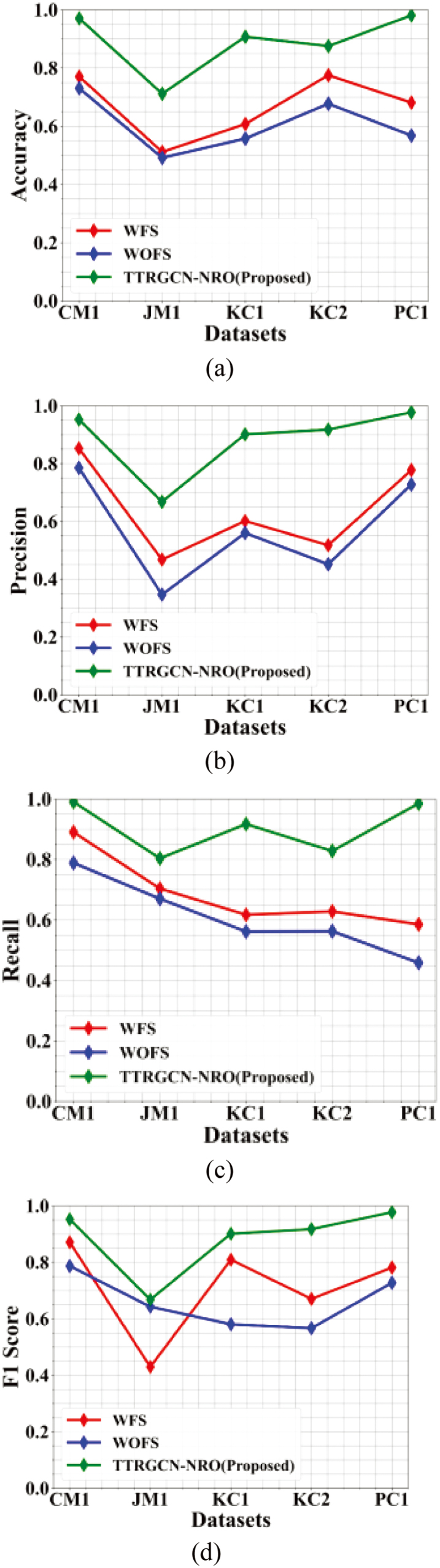 Fig. 7. Performance comparison of defect prediction methods across five datasets based on (a) accuracy, (b) precision, (c) recall, and (d) F1-score.
1).ROC CURVE ANALYSIS
Figure 8 presents the Receiver Operating Characteristic (ROC) curve analysis of different datasets used for SDP, highlighting the true positive rate (TPR) at peak performance. In (a), the CM1 dataset exhibits a high ROC value of 0.99, while (b) shows the JM1 dataset with an ROC value of 0.98. In (c), the KC1 dataset has achieved an ROC value of 0.97. In (d), the KC2 dataset has an ROC value of 0.96. Finally, in (e), the PC1 dataset records an ROC value of 0.99. Overall, the ROC curve analysis demonstrates that the models perform exceptionally well across all datasets, with ROC values consistently above 0.95. The high ROC values indicate that the classification models are effective at distinguishing between defective and non-defective software modules. Among all, the CM1 and PC1 datasets show the highest performance with a near-perfect ROC score of 0.99. JM1 also performs impressively with 0.98, followed by KC1 and KC2. The slight variations in ROC values suggest dataset-specific characteristics. This analysis confirms the reliability of the prediction methods.
 Fig. 8. ROC curve analysis: (a) CM1, (b) JM1, (c) KC1, (d) KC2, and (e) PC1.
2).CONFUSION MATRIX
Figure 9 presents confusion matrices based on actual and predicted values for five SDP datasets. In (a), the CM1 dataset includes 313 no-defect and 322 defect instances, allowing evaluation of models’ performance on a relatively balanced dataset. In (b), the JM1 dataset, with 1018 no-defect and 1277 defect instances, reflects a slightly imbalanced scenario, challenging the model’s defect identification capability. In (c), the KC1 dataset contains 1155 no-defect and 1199 defect instances, providing insights into performance on a nearly balanced and moderately sized dataset. In (d), the KC2 dataset, with 279 no-defect and 256 defect instances, represents a smaller dataset, useful for assessing model generalization on compact data. In (e), the PC1 dataset has 723 no-defect and 745 defect instances, offering a balanced benchmark to evaluate the model’s overall classification accuracy.
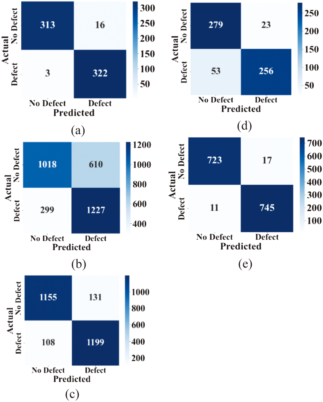 Fig. 9. Confusion matrix with actual and predicted values for the (a) CM1, (b) JM1, (c) KC1, (d) KC2, and (e) PC1 datasets.
E.DISCUSSION
The TTRGCN-NRO model plays a critical role in enhancing SDP by effectively capturing both temporal and spatial dependencies in the data. The dynamic adjacency matrix improves the model’s adaptability to varying data structures. The inclusion of the NRO optimizer accelerates convergence and prevents the model from getting trapped in local minima, resulting in higher precision and recall values across all evaluated datasets. The experimental results consistently show the superiority of TTRGCN-NRO over existing methods across diverse datasets. These findings indicate that the model is robust and reliable for real-world SDP tasks, even under challenges posed by imbalanced and noisy data. The key limitation is that, although the model performs well on benchmark datasets, its effectiveness in large-scale industrial environments with highly heterogeneous data remains untested. The computational complexity of the hybrid architecture could impact scalability for extremely large projects.
F.TRADE-OFF BETWEEN COMPUTATIONAL COST AND PERFORMANCE
When the TTRGCN-NRO method has achieved the superior performance with respect to recall, accuracy, F1-score, and precision, it is important to acknowledge the increased computational complexity introduced by combining transformer-based temporal attention with GCNs and NRO. These enhancements lead to greater training time and higher memory consumption to process iterative optimization and temporal-spatial relationships.
However, the significant performance gain justifies this trade-off. Specifically, the model has achieved over 99% in all major evaluation metrics across all tested datasets, indicating its reliability and robustness in defect prediction. Additionally, the NRO accelerates convergence, reducing the number of training epochs compared to conventional optimization methods like PSO and ACO, as shown in Fig. 6.
The use of RFECV for feature selection and GLOW SMOTE-Density for data balancing helps further to mitigate the computational burden by ensuring balanced class distributions and minimizing input dimensionality. Therefore, the TTRGCN-NRO model introduces extra computational cost, which remains a scalable and efficient choice for high-stakes applications in SDP and risk management.
G.ABLATION STUDY
Table IV shows the ablation study of the performance of different models for SDP. The classical models like KNN [36], Random Forest (RF) [37], and Naïve Bayes (NB) [38] have achieved moderate performance, with F1-scores ranging between 69% and 77%. These models are limited in capturing complex patterns and dependencies inherent in software defect datasets, particularly under imbalance or noise conditions. The RF model performed better, demonstrating the benefit of ensemble learning, but still lagged behind the DL approaches. Although the BiLSTM is capable of modeling temporal dependencies, it showed relatively weak precision and recall due to its limited spatial modeling capabilities. Principal Component-based Support Vector Machine (PC-SVM) performed better in precision and recall but could not match the robustness of our proposed architecture. The BiLSTM model has achieved an accuracy of 88%, with precision and recall values of 57% and 48%, respectively. The PC-SVM has an accuracy of 85.2%, a precision of 83.1%, and a recall of 86%. While the proposed TTRGCN-NRO model significantly outperformed both, achieving the highest accuracy of 99.52%, precision of 98.23%, recall of 97.26%, and F1-score of 97.26%. These results demonstrate that TTRGCN-NRO offers superior capability in accurately detecting software defects with minimal false positives and negatives. The proposed method integrates spatial, temporal, and global temporal features using graph convolution, GRU, and transformer attention layers, respectively. It employs NRO to enhance convergence speed and prediction accuracy. This combination enables robust and precise SDP, outperforming existing methods by a substantial margin.
| Methods | Accuracy (%) | Precision (%) | Recall (%) | F1-score (%) |
|---|---|---|---|---|
| NB | 78.2 | 70.6 | 68.9 | 69.7 |
| RF | 86.7 | 82.4 | 81.1 | 81.7 |
| KNN | 82.4 | 78.2 | 75.5 | 76.8 |
| BiLSTM [ | 88 | 57 | 48 | 53 |
| PC-SVM [ | 85.2 | 83.1 | 86.0 | 76.5 |
| Proposed (TTRGCN-NRO) | 99.52 | 98.23 | 97.26 | 97.26 |
V.CONCLUSION AND FUTURE WORK
This work presented a robust SDP framework that integrated advanced preprocessing techniques for anomaly detection and data balancing. Feature selection is optimized using RFECV, enhancing model relevance and reducing redundancy. The proposed TTRGCN-NRO effectively captured complex spatial and temporal dependencies in software metrics. Hybrid model leveraged graph convolution, GRU, temporal attention, and 1D convolution layers to deliver precise multi-step forecasting. The NRO component accelerated convergence and improved prediction accuracy by directing the search process toward optimal solutions. Experimental evaluations demonstrated that the TTRGCN-NRO outperformed conventional models in defect detection accuracy and generalization. The ROC curve analysis was performed to assess the classification effectiveness of the TTRGCN-NRO across all datasets. The AUC values obtained were 0.99 for CM1, 0.98 for JM1, 0.97 for KC1, 0.96 for KC2, and 0.99 for PC1. These high AUC scores indicated that the model was highly capable of distinguishing between defective and non-defective software modules, with the dataset demonstrating near-perfect classification performance. Through structured preprocessing and hybrid modeling, this approach significantly improved the reliability of SDP. The proposed model enabled software teams to identify potential defect-prone modules early, improving software quality assurance. It supported resource allocation by identifying high-risk areas, thereby reducing both costs and testing efforts. Real-time adaptability made it suitable for large-scale and evolving codebases. The model could be deployed in continuous integration pipelines for dynamic defect tracking.
Future work could explore expanding the model to cross-project defect prediction, which could generalize its applicability further. Incorporating code semantics or developer activity logs may improve contextual understanding. Real-time learning mechanisms could be implemented to adapt to evolving code changes. Investigating federated learning frameworks would allow privacy-preserving defect prediction across organizations. Further optimization of NRO parameters using adaptive learning rates might boost efficiency. Lastly, extending the model to multi-objective optimization can balance defect prediction with other quality attributes like performance and maintainability.