I.INTRODUCTION
During the past decade, data mining has become very popular in the scope of different fields like business, education, finance, and marketing. In the medical domain, data mining is increasingly recognized as an indispensable tool for extracting meaningful patterns from complex datasets. Classification is mainly used for deep insights into patient health conditions and to predict which of the patients might have a disease [1].
Many studies have shown the effectiveness of data mining applications to solve critical healthcare problems. As an example, the kidney datasets are successfully classified to predict the likelihood of kidney failure for kidney disease datasets [2]. Likewise, data mining is used by researchers to classify cancer types, predict fetal heart rate abnormalities using ensemble methods, and estimate the chance of heart stroke [3]. These approaches overcome the shortcomings of manual analysis, reduce diagnostic time, and improve decision-making for the healthcare professional.
Classification is particularly important as a data mining method when we want to predict to which category a given instance belongs. In this process, a dataset is used to train classifiers to build a learning model for performance evaluation. Unfortunately, the attributes in the dataset might be irrelevant, redundant, or noisy and, therefore, dilute the accuracy of the model or induce computational inefficiencies. This is mitigated through the use of a feature selection (FS) step, which reduces the most relevant attributes and discards those that are not necessary [4].
FS methods are broadly categorized into three types:
- 1.Filter Methods - These rank features based on their informational value using algorithms like Relief, Information Gain (IG), Chi-Squared, and Gain Ratio (GR).
- 2.Wrapper Methods - These use specific classifiers to evaluate feature subsets for optimal performance.
- 3.Hybrid Methods - These combine the strengths of both filter and wrapper approaches.
Filter methods rank features based on statistical measures like IG, Chi-Squared, or Relief, independent of the classifier. They are computationally efficient, suitable for high-dimensional datasets, and avoid overfitting. However, they do not consider feature interactions and may result in suboptimal subsets for specific classifiers. Wrapper methods evaluate feature subsets using a particular classifier, optimizing performance [5]. They handle feature interactions well and yield classifier-specific optimal subsets. However, they are computationally expensive, particularly for large datasets, and prone to overfitting, as the evaluation relies heavily on the chosen classifier’s behavior and parameters. There is a need to get the advantage of a wrapper with a filter, as filter methods are computationally efficient. In this research, we propose the similar approach and tested for skin disease.
Class imbalance is another major challenge in medical datasets, where certain classes may dominate others, leading to biased predictions. This issue can be addressed using oversampling techniques such as the Synthetic Minority Oversampling Technique (SMOTE), which generates synthetic instances to balance the dataset [6].
FS has proven instrumental in improving model performance, reducing dimensionality, and minimizing computational costs. For example, FS techniques such as principal component analysis (PCA). It is a dimensionality reduction technique that transforms correlated features into a smaller set of uncorrelated components, preserving most of the dataset’s variance. CFS subset evaluation, which selects subsets of features highly correlated with the target class but uncorrelated with each other, reducing redundancy and Fast Correlation-Based Filter, which identifies a subset of relevant and non-redundant features using Symmetrical Uncertainty (SU) as a ranking metric, have been effectively applied to high-dimensional datasets, including breast cancer and diabetes prediction [7]. These methods help enhance classification accuracy and optimize response time.
Considering the above brief introduction, the problem statement is formulated as follows: diagnosing and classifying skin diseases are critical tasks in dermatology, particularly given the increasing prevalence of skin conditions caused by environmental changes. However, the complexity of medical datasets, characterized by high dimensionality and class imbalance, poses significant challenges to predictive accuracy and computational efficiency. While valuable, existing FS techniques often struggle to address the redundancy and irrelevance of attributes effectively. Moreover, imbalanced datasets lead to biased predictions, further complicating the classification process. To address this,
- •Develop a Novel Framework: Introduce a new FS framework leveraging SU to optimize the feature subset selection process for improved classification accuracy.
- •Address High Dimensionality: Minimize the computational burden by reducing the dataset’s feature space without sacrificing predictive performance.
- •Handle Class Imbalance: Apply techniques like SMOTE to balance the dataset and enhance the robustness of the classification models.
- •Evaluate with Classifiers: Test the proposed framework using popular classifiers such as K-Nearest Neighbour (KNN), JRip, Naive Bayes (NB), and J48, and compare its performance with existing filter-based FS techniques.
- •Provide Quantitative Insights: Rank feature subsets based on classifier performance to identify dermatology datasets’ most effective subset combinations.
To fulfill the above objectives, this research introduces a SU-based framework to form and rank feature subsets, leveraging its ability to measure attribute interdependence. The framework is validated using a benchmark dermatology dataset. Synthetic Minority Oversampling Technique (SMOTE) is applied to address the class imbalance, ensuring a fair evaluation of the subsets. Performance is assessed across multiple classifiers, and results are compared against established FS methods such as Relief, IG, Chi-Squared, and GR. The methodology aims to deliver a scalable, accurate, and efficient solution for predicting skin diseases.
The proposed framework has been tested on a real-time benchmark dermatology dataset, aiming to optimize feature subsets and enhance classification performance. The rest of this article is structured as follows: Section II discusses the dataset and SMOTE results. Section III details the proposed framework. Section IV explains the experimental procedures. Section V presents the results and discussions. Section VI concludes with future recommendations.
II.LITERATURE SURVEY
Whenever it comes to the dermatology, the automation of detecting and diagnosing skin disease has significantly improved by integrating FS and classification techniques. Researchers have recently investigated different techniques to improve the accuracy and speed of skin lesion classification systems. A noteworthy approach is to create an optimal FS paradigm toward skin lesion classification. It can be explained that this is a hybrid method, integrating multiple deep learning models for feature extraction, and removing the redundant information by an entropy-controlled Gray Wolf Optimization (GWO) algorithm. This integrated approach has been evaluated on benchmark dermoscopic datasets and accuracy in classification has been improved on benchmarked dermoscopic datasets and in the range of [8]. A second study offers a wide range of reviews of computer vision methods that address the automated classification of skin diseases. The research highlights the use of machine learning algorithm for FS and dimensionality reduction to maximize the efficiency and effectiveness of skin image analysis. This survey allows for the possibility of incorporating these technologies with dermatology to increase efficacy of diagnostic accuracy [9].
Genetic algorithms (GAs) are used by the authors to select the most relevant features (e.g color, texture features) and eliminate redundant or irrelevant ones of features, in the process of optimizing the FS. Noise, hairs, and air bubbles are removed in preprocessing, and then image is segmented on the basis of homogeneity. The Gray Level Co-occurrence Matrix (GLCM) techniques are used to extract features from images, and those capture properties like energy, entropy, and contrast. An artificial neural network is trained to classify between benign and malignant lesions in the selected features. However, this approach tries to reduce computational complexity without compromising the classification accuracy by selecting features that improve the dermatological diagnostic system [10]
For classification, the authors used statical measures and features extracted from processed images using the GLCM. First comes preprocessing steps: resize, hair removal using BlackHat transformation and inpainting, and Gaussian filtering for noise reduction. The automatic Grabcut technique is used to perform segmentation, improving lesion detection accuracy. Skin lesions are classified into eight categories: melanoma, squamous cell carcinoma, basal cell carcinoma, and others, using three machine learning classifiers: Support Vector Machine (SVM), KNN, and Decision Tree (DT). These classifiers were tested using the ISIC 2019 and HAM10000 datasets. It has been shown through results that the SVM performs better than other classifiers, with 95% accuracy on the ISIC 2019 dataset and 97% on HAM10000 after oversampling over the class imbalance [11].
It is proposed here to take an integrated strategy of reducing dimensionality and then learning in ensembles to classify skin diseases. A feature importance method is applied in the study to find the top 15 significant attributes from the dataset reporting clinical and histopathological features of dermis. This step helps to reduce dataset dimensionality, as well as improve the classification performance with the use of more hyperparameters. Six classifiers are employed in the study: For rapid online learning: (1) Passive Aggressive Classifier; For maximizing class separability; (2) Linear Discriminant Analysis; For distance based neighborhood classification; Radius Neighbors Classifier; and (3) Bernoulli Naïve Bayesian for binary data; Gaussian Naïve Bayesian (NB) for Gaussian data and Extra Tree Classifier a variant of Random Forests [12]. Improving predictive accuracy is undertaken for both the full and reduced datasets with all three ensemble methods: Bagging, AdaBoost, and Gradient Boosting. Yet these strategies frequently require significant computational investment and a fine-tuned hyperparameter optimization to achieve the best performance.
The researchers conducted a comprehensive comparative analysis of deep FS methods for skin lesion classification using various datasets, particularly ISIC 2017 and ISIC 2018. The authors address the challenge of high dimensionality in features extracted from pre-trained deep learning models, which can lead to redundancy and reduced classification efficiency. They evaluate multiple FS techniques, including filter methods (e.g., Relief, Chi-squared, Minimum Redundancy Maximum Relevance (mRMR)), wrapper methods (e.g., GA, Particle Swarm Optimization, GWO), embedded methods (e.g., Random Forest), and dimensionality reduction techniques like PCA. The selected feature subsets are fed into classifiers, primarily KNN, to assess their accuracy, precision, recall, and F1-score performance. The authors’ results indicate that the GWO method outperformed others in accuracy, achieving 83.33% for ISIC 2017 and 93.50% for ISIC 2018. Additionally, the study highlights that combining features from pre-trained models, such as EfficientNet and DenseNet-201, further enhances classification accuracy. This demonstrates the importance of optimal FS in improving computational efficiency and classification performance for skin lesion diagnosis [13]. However, the computational complexity of GWO and its sensitivity to parameter tuning present challenges, especially for high-dimensional datasets.
A general overview of recent research on FS approaches to skin disease classification shows that these methodologies achieve high accuracy and greatly improve computational efficiency. Based on ISIC 2017 and ISIC 2018 datasets, the use of GWO with a wrapper-based approach resulted in 83.33% and 93.50% accuracy in 2023. Making similar contributions using the Whale Optimization Algorithm and Entropy Mutual Information for FS yields 93.4% for the WhaleOptEntropyMutInfo algorithm on HAM10000 and 94.36% for the WhaleOptEntropyMutInfo algorithm on ISIC 2018. Researchers applied the mRMR technique for FS on lung X-ray datasets, with 99.41% accuracy, and skin datasets did not appear in the reported results. An earlier study in 2020 integrated PCA with GWO to optimize features, achieving 80.66% accuracy on the PH2 dataset and 82.00% on ISBI 2017. Another notable approach from 2019 employed Biomedical Deep Feature Selection with ensemble techniques for multiple datasets, achieving 94% accuracy for skin lesions and 93% for leukemia. These studies underscore the growing importance of FS methods such as GWO, mRMR, and hybrid algorithms in improving skin disease classification accuracy across diverse datasets.
A comparative study on deep FS methods highlighted that wrapper techniques, such as GWO, outperform filter and embedded methods in accuracy. Yet, these methods often involve high computational costs and are prone to overfitting, particularly in small or imbalanced datasets. Despite these challenges, FS and classification advancements continue to make significant strides in dermatology, albeit with room for improvement in addressing scalability, computational efficiency, and dataset generalization.
In this research, to draw the benefits of wrapper, we proposed a novel features selection framework using filter approaches, which will be discussed in the next section.
III.METHODOLOGY
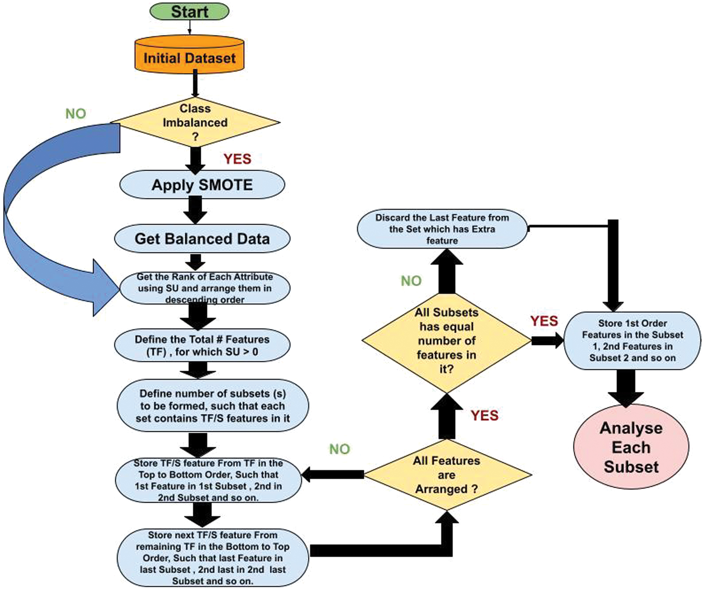
As per Fig. 1, the proposed methodology in this research introduces an ensemble FS approach to enhance classification accuracy for dermatological datasets. The process begins with a preprocessing stage, where a dermatology dataset from the UCI Machine Learning Repository is balanced using the SMOTE to address class imbalance. Synthetic Minority Oversampling Technique (SMOTE) uses the KNN algorithm to synthesize artificial instances, ensuring equitable distribution across all classes [14]. Features are extracted, and their SU values are computed to measure the interdependence between features and class labels [15]. SU is defined as
IG is Information Gain
H(A) is the Entropy of A
H(B) is the Entropy of B
Symmetrical Uncertainty (SU) was selected as the core filter metric in our framework due to its balance between informativeness and computational efficiency. Unlike mutual information, SU normalizes the IG by the entropy of both the feature and the class, making it symmetric and thus more suitable when dealing with multi-class problems such as dermatological classification. Compared to mRMR, which optimizes both relevance and redundancy but requires pairwise feature evaluations (resulting in quadratic time complexity), SU operates independently per feature, significantly reducing computational load. This makes SU particularly advantageous for high-dimensional datasets where speed and scalability are crucial. Additionally, SU is less sensitive to class imbalance and provides stable feature rankings even under noisy data conditions.
To minimize dimensionality, features with zero SU values are discarded, and the remaining features are ranked based on SU values. The ranked features are divided into subsets, each containing a predefined number of features. The feature grouping process employs a systematic approach, ensuring non-redundant distribution of features across subsets.
Each subgroup is evaluated using four classifiers: KNN, JRip, NB, and J48. These classifiers assess the predictive accuracy of each subset. Additionally, the performance of the proposed framework is compared against existing filter-based FS techniques, such as Relief, IG, Chi-Squared Attribute Evaluator (Chi), and GR Attribute Evaluator. The ranking is assigned to each subset based on its classification performance across the models.
K-Nearest Neighbor (KNN) is a simple, instance-based machine learning algorithm used for classification and regression. It classifies a data point based on the majority class of its KNN in the feature space. Distance metrics like Euclidean or Manhattan distances are used to determine proximity. It works well with smaller datasets but can be computationally expensive for larger datasets [16].
JRip is an implementation of the Repeated Incremental Pruning to Produce Error Reduction algorithm. It generates rule-based classification models, where the dataset is divided into positive and negative classes, and rules are iteratively optimized to improve accuracy. It is particularly efficient for datasets with categorical attributes and provides interpretable results [17]. Naive Bayes (NB) is a probabilistic classifier based on Bayes’ Theorem, which assumes that all features are independent given the class label. Despite its simplicity, it works well for many real-world datasets, particularly for text classification and problems with categorical features. It is computationally efficient and interpretable [18].
J48 is an implementation of the C4.5 DT algorithm. It constructs a DT based on IG or GR to split attributes at each node [19]. The resulting tree can be used for classification, offering a balance between performance and interpretability. It handles both numerical and categorical data effectively [20].
A.RATIONALE FOR CLASSIFIER DIVERSITY
Each classifier processes feature subsets differently. KNN relies on distance metrics and is sensitive to feature scaling and redundancy, JRip generates interpretable rule sets based on attribute discrimination, NB assumes conditional independence and evaluates statistical relevance, while J48 constructs tree-based decision paths guided by IG. By evaluating feature subsets across these heterogeneous classifiers, we gain robust insights into how well the subsets generalize across different algorithmic principles. This approach minimizes the risk of method-specific overfitting and strengthens the external validity of the proposed framework. The observed consistent performance improvements across classifiers further validate the versatility and robustness of the feature subsets generated using SU.
Relief is a filter-based method that ranks features based on their ability to distinguish between instances of different classes [21]. It evaluates the relevance of a feature by measuring how well it separates neighboring instances from the same and different classes [22]. IG measures the reduction in entropy after a feature is used to split the data. It quantifies how much information a feature contributes to predicting the class label. Features with higher IG are considered more relevant for classification [23]. Chi evaluates the dependency between a feature and the class label by calculating the Chi-squared statistic. Features with a higher Chi-squared value are considered more dependent on the class and hence more relevant for classification [24]. Gain Ratio (GR) is a normalized version of IG that accounts for the bias IG might introduce when selecting features with many unique values. It is used in DT algorithms like C4.5 to ensure a more balanced FS process [25].
The framework is tested on imbalanced and balanced datasets, forming subsets with varying feature counts (e.g., 3, 4, or 5 subsets). This evaluation allows for a comparative analysis of the proposed method’s efficiency in reducing dimensionality while maintaining or improving classification accuracy. The proposed methodology demonstrates its strength in achieving significant accuracy improvements and computational efficiency for dermatological classification tasks.
The pseudo-code below explains the process outlined in the flowchart in a structured, step-by-step manner. It ensures that features are assigned to subsets alternately (top to bottom and bottom to top) and validates the final subsets for equal distribution of features.
Pseudocode:
START
// Step 1: Load Dataset
Input: Initial Dataset
// Step 2: Check for Class Imbalance
IF Class is Imbalanced THEN
Apply SMOTE to balance the dataset
Get the Balanced Dataset
END IF
// Step 3: Rank Features
FOR each feature in the dataset DO
Calculate Symmetrical Uncertainty (SU)
Rank features in descending order of SU
END FOR
Discard features with SU = 0
Define Total Features (TF) as features with SU > 0
// Step 4: Define Subsets
Input: Number of Subsets (S)
Features per Subset = TF/S
// Step 5: Assign Features to Subsets
WHILE All Features are not Assigned DO
// Top to bottom Assignment
FOR i = 1 TO S DO
Assign next available feature to Subset[i]
END FOR
// Bottom to Top Assignment
FOR i = S TO 1 DO
Assign next available feature to Subset[i]
END FOR
END WHILE
// Step 6: Check and Enforce Equal Distribution
FOR each Subset[i] DO
IF Subset[i] contains more than Expected_Feature_Count THEN
Remove last-added feature from Subset[i]
END IF
END FOR
// Step 7: Store and Output Subsets
Store features in respective Subsets
Output: Subsets of Features with Equal Distribution
END
IV.EXPERIMENTAL RESULTS
The dataset utilized in this study is the dermatology dataset obtained from the UCI Machine Learning Repository [26]. The dataset consists of 366 instances and 34 attributes, with each record classified into one of six disease categories: psoriasis, seborrheic dermatitis, lichen planus, pityriasis rosea, chronic dermatitis, and pityriasis rubra pilaris. Each disease is represented by a class label (1–6). Table I details the class distribution, showing a significant class imbalance, with Class 1 (psoriasis) comprising 30.6% of the total records, while Class 6 (pityriasis rubra pilaris) accounts for only 5.46%. To address the class imbalance, the SMOTE was applied. Synthetic Minority Oversampling Technique (SMOTE) synthesized additional instances for minority classes based on the KNN algorithm, using K = 5 and a predefined percentage for each class. This preprocessing step increased the dataset to 686 instances, creating a near-balanced dataset, as shown in Table I.
Table I. Dataset distribution before and after balancing
| Class Code | Disease Name | Instances (Before SMOTE) | Percentage (Before SMOTE) | Instances (After SMOTE) | Percentage (After SMOTE) |
|---|---|---|---|---|---|
| 1 | Psoriasis | 112 | 30.60% | 112 | 16.32% |
| 2 | Seborrheic Dermatitis | 61 | 16.66% | 122 | 17.79% |
| 3 | Lichen Planus | 72 | 19.67% | 111 | 16.18% |
| 4 | Pityriasis Rosea | 49 | 13.38% | 107 | 15.60% |
| 5 | Chronic Dermatitis | 52 | 14.20% | 114 | 16.62% |
| 6 | Pityriasis Rubra Pilaris | 20 | 5.46% | 120 | 17.49% |
As per the proposed method, Table II describes the dataset SU score and rank of each feature by the filtered methods of the primary dataset (imbalanced).
Table II. SU score and rank of each feature by the filtered methods of the primary dataset
| Rank (SU) | SU Score | FNo. of (SU) | FNo. of (IG) | FNo. of (Chi) | FNo. of (Rel) | FNo. of (GR) |
|---|---|---|---|---|---|---|
| 1 | 0.4778 | 21 | 21 | 33 | 21 | 12 |
| 2 | 0.4672 | 22 | 20 | 29 | 33 | 29 |
| 3 | 0.4489 | 20 | 22 | 12 | 22 | 33 |
| 4 | 0.4328 | 33 | 33 | 27 | 20 | 27 |
| 5 | 0.4291 | 29 | 29 | 15 | 28 | 15 |
| 6 | 0.427 | 27 | 27 | 31 | 27 | 31 |
| 7 | 0.426 | 12 | 12 | 6 | 29 | 25 |
| 8 | 0.4188 | 25 | 25 | 25 | 6 | 6 |
| 9 | 0.4147 | 6 | 6 | 8 | 12 | 8 |
| 10 | 0.3944 | 8 | 8 | 22 | 16 | 22 |
| 11 | 0.3739 | 15 | 9 | 21 | 25 | 9 |
| 12 | 0.3288 | 9 | 16 | 30 | 8 | 30 |
| 13 | 0.3197 | 28 | 15 | 20 | 15 | 20 |
| 14 | 0.2979 | 16 | 28 | 7 | 9 | 7 |
| 15 | 0.2904 | 10 | 10 | 24 | 4 | 24 |
| 16 | 0.28 | 24 | 24 | 10 | 14 | 10 |
| 17 | 0.2505 | 14 | 14 | 28 | 10 | 28 |
| 18 | 0.2244 | 5 | 5 | 34 | 24 | 34 |
| 19 | 0.2159 | 31 | 26 | 9 | 30 | 9 |
| 20 | 0.2094 | 26 | 3 | 14 | 3 | 14 |
| 21 | 0.1868 | 7 | 31 | 16 | 26 | 16 |
| 22 | 0.1825 | 30 | 19 | 5 | 19 | 5 |
| 23 | 0.1726 | 23 | 23 | 23 | 7 | 23 |
| 24 | 0.1692 | 3 | 7 | 26 | 11 | 26 |
| 25 | 0.1447 | 34 | 30 | 11 | 2 | 11 |
| 26 | 0.1441 | 19 | 2 | 4 | 31 | 4 |
| 27 | 0.1341 | 4 | 4 | 3 | 18 | 3 |
| 28 | 0.1301 | 2 | 34 | 19 | 23 | 19 |
| 29 | 0.1066 | 11 | 11 | 2 | 13 | 2 |
| 30 | 0.0641 | 1 | 1 | 13 | 17 | 17 |
| 31 | 0.0597 | 13 | 13 | 1 | 34 | 1 |
| 32 | 0.0495 | 17 | 18 | 17 | 1 | 13 |
| 33 | 0.0483 | 18 | 17 | 18 | 32 | 18 |
| 34 | 0 | 32 | 32 | 32 | 32 | 32 |
Total features whose SU > 0 (TF): 33, the last feature has zero value, so it is removed from the consideration. If we want to form 4 subsets, then each subset contains 8 features (33/4 = 8). Table III is a simple example of how the features are formed in each subset when 4 subsets are formed as per the proposed methodology.
Table III. Features formed by the proposed method when S = 4
| 21 | 25 | 6 | 24 | 14 | 3 | 34 | 17 | 18 | ||
| 22 | 12 | 8 | 10 | 5 | 23 | 19 | 13 | |||
| 20 | 27 | 15 | 16 | 31 | 30 | 4 | 1 | |||
| 33 | 29 | 9 | 28 | 26 | 7 | 2 | 11 | |||
| Top to Bottom | Bottom to Top | Top to Bottom | Bottom to Top | Top to Bottom | Bottom to Top | Top to Bottom | Bottom to Top | Top to Bottom |
From Table III above, Subset IS41 contains an additional feature, i.e., feature ID 18, which must be discarded to maintain equal distribution across all subsets. Once this adjustment is made, the features are reorganized based on their order of assignment: first-order features are grouped into IS41 (21, 25, 6, 24, 14, 3, 34, 17), second-order features into IS42 (22, 12, 8, 10, 5, 23, 19, 13), third-order features into IS43 (20, 27, 25, 26, 32, 30, 4, 1), and fourth-order features into IS44 (33, 29, 9, 28, 26, 7, 2, 11). As each subset has 8 features in it. The top 8 features derived from the existing methods are shown here. IG * (21, 20, 22, 33, 29, 27, 12, 25), GR * (12, 29, 33, 15, 27, 31, 6, 25), Chi-Squared * (33, 29, 27, 12, 15, 31, 25, 6), and Relief * (21, 33, 22, 20, 28, 27, 29, 6).
To evaluate and analyze the effectiveness of the proposed framework, we considered scenarios with S = 3 and 5. The features are redistributed into different subsets based on the number of subsets (S) selected for the experiments. For S = 3, each subset contains more features due to a smaller number of groups, while for S = 5, the subsets are more compact, each containing fewer features. For S = 4, the subsets balance the trade-off between group size and feature relevance. This hierarchical grouping demonstrates the adaptability of the proposed framework to varying configurations, ensuring optimal feature utilization for different classification needs. Across all scenarios, features ranked highly by the proposed method strongly overlap with those identified by existing FS methods (e.g., IG, GR, Chi-Squared, and Relief). For instance, features such as 21, 33, 29, 27, and 12 consistently appear in the top ranks across the IG, Chi-Squared, and Relief methods. This overlap validates the efficacy of the proposed framework in identifying features critical for classification accuracy. While the proposed framework incorporates features ranked highly by existing methods, it also introduces new feature subsets that enhance classifier performance. For example, 19, 14, and 17 features are included in subsets (e.g., IS31, IS44) due to their utility within specific subsets, though they may not rank as highly in existing methods.
The same framework was also applied to the balanced dataset obtained through an oversampling technique. Symmetrical Uncertainty (SU) was used to rank each attribute on the balanced dataset. The ranking results from SU are as follows: 21, 31, 7, 15, 33, 29, 27, 9, 12, 25, 6, 30, 8, 20, 22, 5, 28, 34, 10, 14, 16, 26, 11, 24, 4, 3, 2, 23, 19, 1, 18, 17, 13, 32.
All attributes in the balanced dataset had SU values greater than zero and were therefore included in the subset formation process. Subsets of features were formed with S=3, S=4, and S=5 as shown in Table IV. The same experimental procedures conducted on the imbalanced dataset were repeated on the balanced dataset to assess and compare performance.
Table IV. Subsets of features over Balanced dataset
| S Value | Subset ID | Features in Subset |
|---|---|---|
| 3 | BS31 | 10, 24, 4, 1, 18, 21, 29, 27, 30, 8, 34, |
| BS32 | 31, 33, 11, 3, 19, 17,9, 6, 20, 28, 14 | |
| BS33 | 7, 15, 12, 25, 22, 5, 16, 26, 2, 23, 13 | |
| Information Gain | 21, 9, 7, 31, 20, 28, 25, 15, 33, 29, 27 | |
| Gain Ratio | 21, 7, 25, 31, 33, 29, 27, 12, 9, 15, 6 | |
| Chi -Squared | 31, 12, 29, 33, 27, 15, 6, 8, 22, 30, 25 | |
| Relief | 33, 21, 28, 29, 27, 31, 6, 7, 15, 9, 12 | |
| 4 | BS41 | 21, 9, 12, 5, 28, 24, 4, 17 |
| BS42 | 31, 27, 25, 22, 34, 11, 3, 18 | |
| BS43 | 7, 29, 6, 20, 10, 26, 2, 1 | |
| BS44 | 15, 33, 30, 8, 14, 16, 23, 19 | |
| Information Gain | 21, 9, 7, 31, 20, 28, 25, 15 | |
| Gain Ratio | 21, 7, 25, 31, 33, 29, 27, 12 | |
| Chi-Squared | 31, 12, 29, 33, 27, 15, 6, 8 | |
| Relief | 33, 21, 28, 29, 27, 31, 6, 7 | |
| 5 | BS51 | 21, 25, 6, 14, 16, 1 |
| BS52 | 31, 12, 30, 10, 26, 19 | |
| BS53 | 15, 33, 9, 20, 8, 24 | |
| BS54 | 7, 29, 22, 11, 4, 23 | |
| BS55 | 34, 28, 27, 2, 3, 18 | |
| Information Gain | 21, 9, 7, 31, 20, 28 | |
| Gain Ratio | 21, 7, 25, 31, 33, 29 | |
| Chi-Squared | 31, 12, 29, 33, 27, 15 | |
| Relief | 33, 21, 28, 29, 27, 31 |
Indicate Top 11 features selected by the existing methods;
Top 8 features selected by the existing methods;
Top 6 features selected by the existing methods.
The choice of S = 3, 4, and 5 for feature subset grouping was guided by the need to balance computational efficiency and classification performance. These values allowed the subsets to be sufficiently small for interpretability while retaining a diverse mix of high-ranked features.
V.DISCUSSION
The performance of each classifier (KNN, JRip, NB, and J48) is evaluated for every subset of features, and their ranks are determined based on classification accuracy. Each classifier’s rank for a specific subset is denoted using a “/” (slash), representing a comparison of how well each subset performed relative to others for the same classifier. The evaluation process includes testing the subsets formed for different configurations (e.g., S = 3, S = 4, and S = 5) over both imbalanced and balanced datasets. The accuracy is computed for every subset-classifier combination. This comprehensive ranking system ensures a fair comparison across subsets, enabling an analysis of the relative strengths of each feature grouping for different classifiers.
The performance of each classifier against the subsets of features is evaluated for both imbalanced and balanced datasets as per Table V. Each subset’s rank by a specific classifier is denoted with a slash (e.g., 84.42/4), indicating its accuracy and relative ranking among the subsets. IS31 Subset showed improved performance with JRip (86.06/1) and registered consistent rankings for KNN, NB, and J48, achieving an accuracy of 84.42/4, 90.43/2, and 87.43/2, respectively. IS32 Subset outperformed others, registering the best performance across most classifiers: KNN (87.43/1), NB (90.71/1), and J48 (88.52/1). Demonstrates the highest classification potential for imbalanced data. IS33 Subset ranked lower in comparison, achieving its best performance with KNN (85.71/3) but lower rankings for other classifiers.
Table V. Performance analysis with 3 Subsets
| IS31 | IS32 | IS33 | CHI | GR | IG | REL | ||
| 84.42/4 | 85.71/3 | 85.79/2 | 83.06/5 | 80.05/7 | 80.32/6 | |||
| 85.24/2 | 82.24/5 | 83.6/3 | 82.78/4 | 64.48/7 | 72.4/6 | |||
| 90.43/2 | 84.42/4 | 85.51/3 | 83.87/5 | 79.23/6 | 79.23/7 | |||
| 87.43/2 | 83.06/4 | 83.33/3 | 81.69/5 | 78.68/6 | 74.86/7 | |||
| BS31 | BS32 | CHI | GR | IG | REL | |||
| 88.92/3 | 92.27/2 | 84.83/6 | 82.94/7 | 87.60/4 | 87.60/5 | |||
| 85.56/3 | 91.10/2 | 84.40/6 | 82.50/7 | 85.42/4 | 85.13/5 | |||
| 81.91/6 | 86.29/2 | 83.66/5 | 81.04/7 | 86.15/3 | 85.56/4 | |||
| 87.90/3 | 92.27/2 | 83.38/6 | 82.50/7 | 85.56/4 | 85.56/5 |
BS31 Subset demonstrated moderate improvement across classifiers with KNN (88.92/3), JRip (85.56/3), and J48 (87.90/3). BS32 Subset achieved exceptional results across classifiers, maintaining high accuracy: KNN (92.27/2), NB (86.29/2), and J48 (92.27/2). This subset stands out for balanced data with reliable performance across classifiers. BS33 Subset dominated with the highest performance for all classifiers: KNN (97.66/1), JRip (97.08/1), NB (97.81/1), and J48 (97.52/1). Clearly, the most robust subset for the balanced dataset.
Compared to existing methods, subsets like IS32 and BS33 demonstrated superior performance over existing methods such as Chi-Squared (CHI), GR, IG (IG), and Relief (REL). For example, CHI and GR consistently ranked lower in balanced datasets with NB (CHI: 83.66/5, GR: 81.04/7) and KNN (CHI: 84.83/6, GR: 82.94/7). IS31 showed noticeable improvement with JRip (86.06/1), while IS32 registered high accuracy for KNN, NB, and J48, outperforming existing methods. The same is shown in Fig. 2.
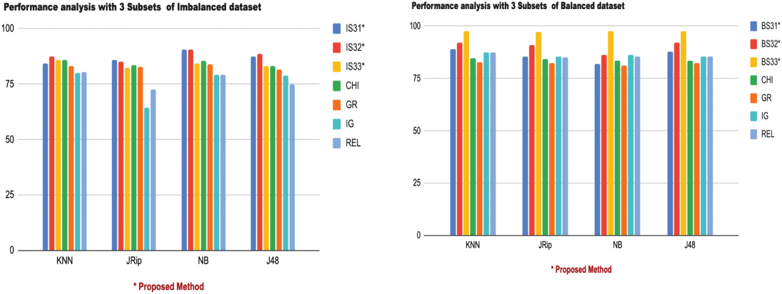 Fig. 2. Graphical representation of performance analysis with 3 Subsets.
The performance of each classifier was evaluated for subsets IS41, IS42, IS43, IS44 (imbalanced dataset) and BS41, BS42, BS43, BS44 (balanced dataset) as shown in Table VI. On the imbalanced dataset, IS43 achieved the highest performance across all classifiers, with rankings of KNN (88.25/1), JRip (87.97/1), NB (91.25/1), and J48 (91.53/1), indicating its superior classification ability. IS41 performed well with JRip (84.15/2) and consistently ranked with other classifiers. Subsets IS42 and IS44 showed moderate results, with IS44 performing better with NB (86.33/3) and J48 (84.15/3).
Table VI. Performance analysis with Subset 4
| ID | IS41 | IS42 | IS44 | CHI | GR | IG | REL | ||
| 82.51/3 | 80.6/4 | 84.15/2 | 69.12/7 | 69.12/7 | 75.95/6 | 78.14/5 | |||
| 84.15/2 | 68.57/5 | 82.51/3 | 68.03/6 | 68.03/6 | 59.83/7 | 75.13/4 | |||
| 86.61/2 | 80.32/4 | 86.33/3 | 69.12/7 | 69.12/7 | 74.86/6 | 78.41/5 | |||
| 86.06/2 | 80.87/4 | 84.15/3 | 68.57/7 | 68.57/7 | 75.95/6 | 76.22/5 | |||
| BS42 | BS43 | BS44 | CHI | GR | IG | REL | |||
| 73.76/6 | 87.02/4 | 88.48/2 | 73.46/7 | 65.59/8 | 87.17/3 | 77.84/5 | |||
| 73.17/6 | 88.48/3 | 88.75/2 | 72.15/7 | 67.49/8 | 85.27/4 | 78.13/5 | |||
| 86.44/2 | 72.01/6 | 81.19/4 | 68.95/7 | 65.59/8 | 85.86/3 | 73.32/5 | |||
| 73.17/6 | 88.62/2 | 88.48/3 | 72.59/7 | 67.20/8 | 85.86/4 | 74.48/5 |
On the balanced dataset, BS41 outperformed all subsets with rankings of KNN (91.25/1), JRip (91.39/1), and J48 (91.54/1), while BS44 excelled with NB (87.12/1). BS43 demonstrated competitive performance, achieving KNN (87.02/4), JRip (88.48/3), and J48 (88.62/2). BS42, however, consistently ranked the lowest, indicating a weaker feature set for classification.
Compared to existing methods, the proposed subsets significantly outperformed. For instance, in the imbalanced dataset, Chi-Squared and GR ranked the lowest across all classifiers, with KNN (CHI: 69.12/7, GR: 69.12/7) and J48 (CHI: 68.57/7, GR: 68.57/7). Similarly, these methods maintained their lower rankings on the balanced dataset, with KNN (CHI: 73.46/7, GR: 65.59/8) and NB (CHI: 68.95/7, GR: 65.59/8). The subsets like IS43 and BS41 showcased remarkable performance, demonstrating the robustness of the proposed framework for both datasets. The results also highlight the ability to enhance classification accuracy while reducing feature redundancy. The same is shown graphically in Fig. 3.
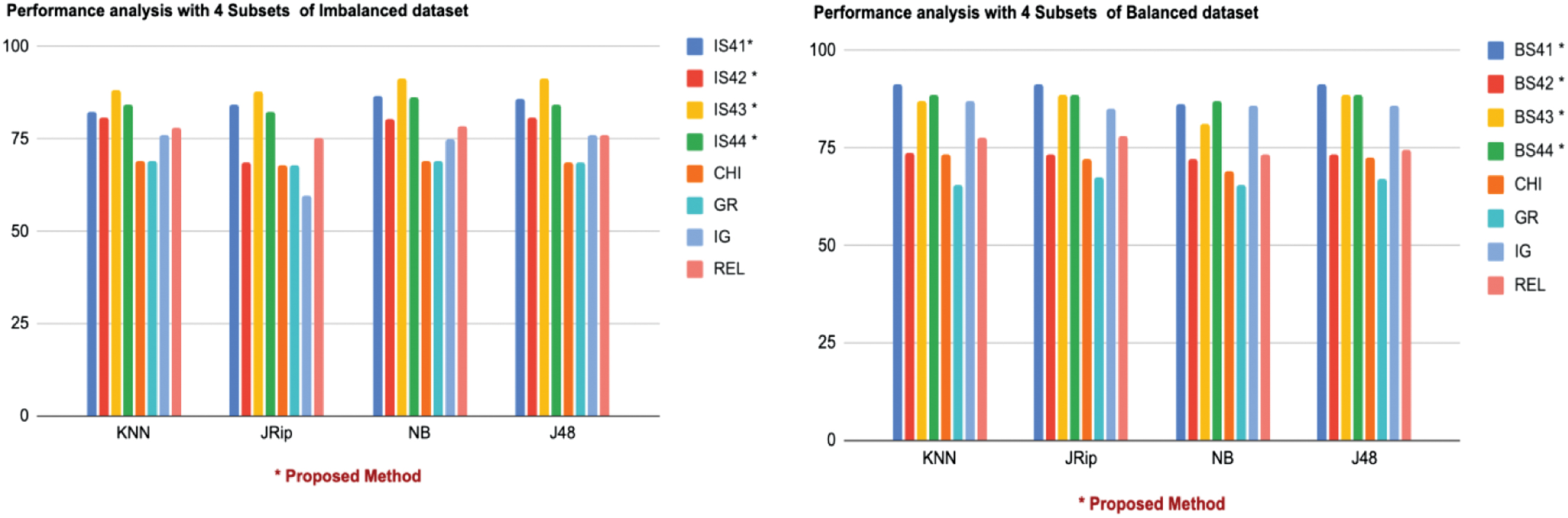 Fig. 3. Graphical representation of performance analysis with 4 Subsets.
The performance evaluation of subsets IS51, IS52, IS53, IS54, IS55 (imbalanced dataset) and BS51, BS52, BS53, BS54, BS55 (balanced dataset) against classifiers KNN, JRip, NB, and J48 reveals significant insights into the strengths of the proposed framework, as shown in Table VII. On the imbalanced dataset, IS53 demonstrated the best overall performance, achieving top ranks for KNN (86.61/1), JRip (86.06/1), and J48 (87.7/1), while performing strongly with NB (87.43/2). Similarly, IS51 performed exceptionally well, ranking first for NB (87.97/1) and J48 (87.7/1) while securing second place for both KNN (85.51/2) and JRip (85.51/2). In contrast, subsets like IS54 displayed moderate performance with consistent rankings of 4th across classifiers, and IS55 consistently ranked lowest, with weak scores such as KNN (64.2/8) and JRip (53.82/8).
Table VII. Performance analysis with Subset 5
| IS51 | IS52 | IS53 | IS54 | IS55 | CHI | GR | IG | REL | ||
| 85.51/2 | 69.67/6 | 76.77/4 | 64.2/8 | 69.12/7 | 69.12/7 | 76.22/5 | 77.59/3 | |||
| 85.51/2 | 54.64/7 | 70.49/4 | 53.82/8 | 69.12/5 | 69.12/5 | 59.28/6 | 71.85/3 | |||
| 70.21/6 | 87.43/2 | 76.5/4 | 65.3/8 | 69.12/7 | 69.12/7 | 74.86/5 | 78.41/3 | |||
| 70.76/5 | 74.31/4 | 65.4/7 | 68.85/6 | 68.85/6 | 76.22/3 | 76.77/2 | ||||
| BS51 | BS52 | BS53 | BS54 | BS55 | CHI | GR | IG | REL | ||
| 78.71/2 | 71.57/7 | 69.82/8 | 76.38/4 | 73.61/6 | 67.20/9 | 75.51/5 | 76.53/3 | |||
| 80.17/2 | 71.20/6 | 66.47/8 | 72.59/4 | 72.44/5 | 67.34/7 | 72.44/5 | 76.53/3 | |||
| 71.28/6 | 72.30/4 | 70.11/7 | 73.90/3 | 69.97/8 | 65.59/9 | 75.05/2 | 72.15/5 | |||
| 80.75/2 | 72.15/7 | 67.93/8 | 74.05/5 | 72.59/6 | 67.20/9 | 74.34/4 | 74.92/3 |
On the balanced dataset, BS54 outperformed all other subsets, ranking first across all classifiers, including KNN (81.63/1), JRip (81.77/1), NB (77.69/1), and J48 (81.04/1). BS51 also delivered strong performance, especially with JRip (80.17/2) and J48 (80.75/2), though it ranked lower with NB (71.28/6). Subsets like BS55 exhibited moderate results, achieving third place with NB (73.90/3) but dropping to fifth with J48 (74.05/5). Conversely, BS52 and BS53 consistently ranked among the lowest-performing subsets, with BS53 registering its weakest scores for KNN (69.82/8) and JRip (66.47/8).
The proposed subsets were either comparable or superior to existing methods. On the imbalanced dataset, the order of CHI and GR is lowest and they had exactly the same results as KNN (69.12/7), J48 (68.85/6). Likewise, on the balanced dataset, same as all the rest, KNN achieved (73.61/6, 67.20/9) and NB (69.97/8, 65.59/9) as well. Although higher than CHI and GR, REL did not meet the proposed subsets.
Subsets BS54 (from the balanced dataset) and IS53 (from the imbalanced dataset) consistently achieved the highest classification accuracy across all four classifiers (KNN, JRip, NB, and J48), as shown in Fig. 4. This consistent outperformance can be attributed to the strategic inclusion of top-ranked features such as 7, 29, 22, and 11 in BS54 and 15, 33, 9, and 20 in IS53. Many of these features also appear in the top positions across multiple filter methods (e.g., SU, IG, and GR), indicating their strong individual relevance.
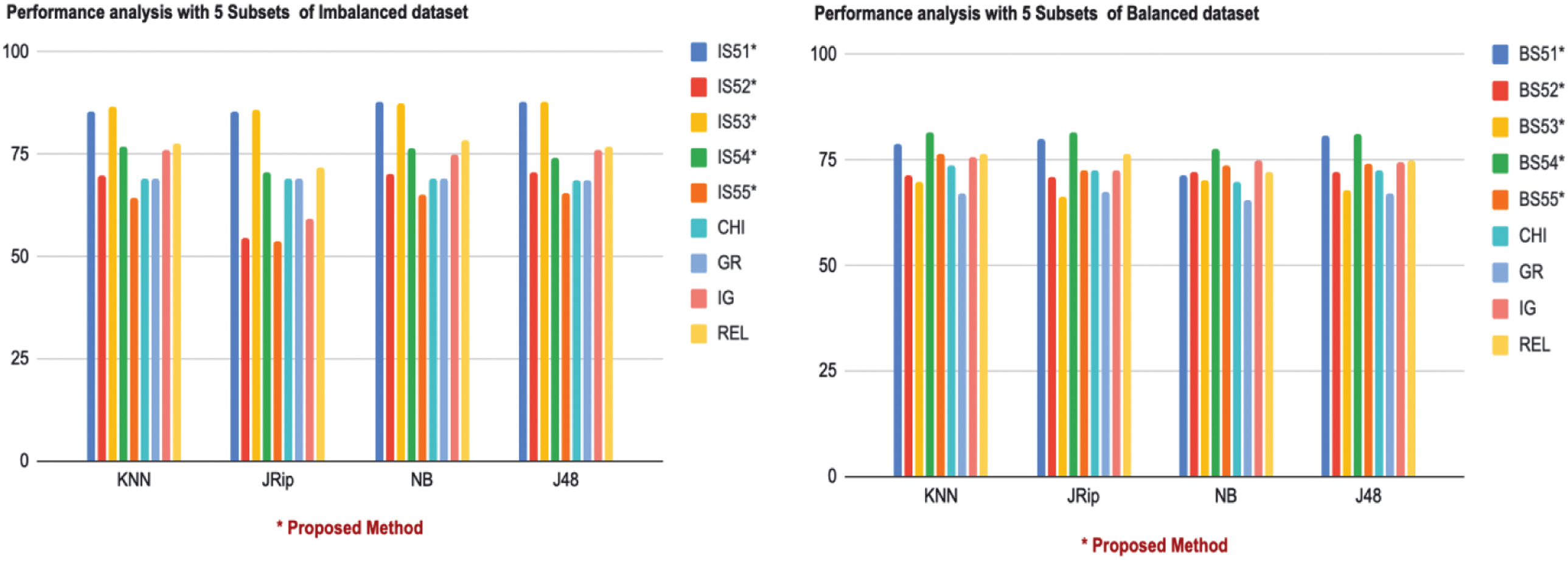 Fig. 4. Graphical representation of performance analysis with 5 Subsets.
The primary contribution of this research is the development of a novel feature subset selection and ranking framework leveraging SU to address challenges in high-dimensional datasets and class imbalance, particularly in dermatological classification tasks. The framework combines the computational efficiency of filter-based methods with the feature optimization capabilities of wrapper approaches. Features are ranked and grouped systematically into subsets, which are then evaluated using multiple classifiers (KNN, JRip, NB, and J48). This approach not only reduces dimensionality but also enhances classification accuracy compared to existing filter-based FS techniques, as demonstrated on a benchmark dermatology dataset.
While the framework shares some similarities with ensemble methods, such as combining the strengths of different subsets and classifiers, it is fundamentally different. The framework focuses on feature subset formation and selection, optimizing input data for classifiers rather than combining classifier predictions like traditional ensemble approaches. However, its ability to leverage diverse feature subsets and multiple classifiers contributes to its enhanced performance, resembling the robustness typically seen in ensemble techniques. This indicates that systematic feature grouping and ranking, akin to ensembling data inputs, can significantly boost classification outcomes.
While wrapper-based methods like J48 with BestFirst search often deliver strong classification accuracy, they do so at a much higher computational cost. In contrast, our proposed SU-based method eliminates the need for repeated classifier training during subset search, resulting in significantly reduced runtime and memory usage.
Why the Results are Better:
- 1.Improved Feature Ranking: SU effectively measures the interdependence between features and class labels, ensuring that the selected features are highly relevant for classification.
- 2.Subset Formation: The systematic grouping of features into subsets reduces redundancy and ensures balanced distribution across subsets, enhancing predictive performance.
- 3.Class Imbalance Handling: The application of the SMOTE addresses class imbalance, improving classifier performance for minority classes.
- 4.Comprehensive Evaluation: The framework was rigorously tested with multiple classifiers and configurations (e.g., varying subset sizes), ensuring robust validation of results.
- 5.Comparison with Existing Methods: By outperforming existing methods (Relief, IG, Chi-Squared, and GR), the proposed framework demonstrates its superiority in identifying critical features for improved classification accuracy.
The current SU-based framework evaluates features individually and does not capture multivariate interactions. In future work, we plan to incorporate multivariate methods like mRMR or CFS and optimization algorithms such as GAs to account for feature dependencies. These enhancements will improve the framework’s robustness and ability to handle complex, high-dimensional medical datasets more effectively.
VI.CONCLUSION
In this study, a novel framework for feature subset selection and ranking was proposed. The framework enables the creation of “S” subsets, each comprising a minimal, non-redundant set of features. These subsets were evaluated using four diverse classifiers—JRip, J48, NB, and KNN—and compared against traditional filter-based FS methods. Subsets were ranked based on classification accuracy, and the results revealed that certain subsets consistently outperformed existing methods, achieving superior predictive accuracy.
This confirms that the proposed methodology offers a flexible and computationally efficient approach to forming high-quality feature subsets, especially when specific prediction accuracy requirements are desired. Although the framework’s performance may vary depending on the dataset, its adaptability shows promising generalization.
For future work, the framework can be extended to other datasets and domains to validate its generalizability. Its performance may be further enhanced by integrating advanced classifiers such as ensemble models (e.g., Random Forest, Gradient Boosting) or deep learning architectures. Optimization techniques like GAs or Particle Swarm Optimization can also be employed to refine feature subsets more effectively. Additionally, reducing computational overhead will allow broader application to large-scale and real-time datasets. The framework can be strengthened for noisy data by introducing adaptive mechanisms that dynamically determine the optimal number of subsets (S) based on dataset characteristics. These improvements would enhance the framework’s robustness, efficiency, and applicability to a wider range of real-world problems.