I.INTRODUCTION
Ensuring security and safety of the public is one of the greatest challenges and an indispensable instrument in maintaining the tranquility and solidarity in this contemporary society. Urgency for deploying such surveillance systems in densely populated areas such as public transport hubs, pilgrimage, crowded city centers, and social events in urban areas [1] finds its demand with its immediate effect. Such environments witness a high degree of complexity and assessment in terms of head count, motion direction, acceleration, and determination of the trajectories of the individuals in the varied crowd scenarios. Detection of the unusual occurrences of criminal and violent acts such as robbery, theft, fights, vandalism, suspicious behavior, accidents, and medical emergencies remains a challenging task even with its advanced statistical dynamics in classifying, detecting, and tracking it in precarious conditions. These real-time events are categorized as anomalies in crowded environments [2]. Controlling the crowd and minimizing distress among the people can be done if the bizarre activities are detected and reported early to maintain public safety. In such emergency situations, conventional approaches for anomaly identification frequently flounder in terms of rate of detection, predetermination of computational complexity, and frame processing. In order to improve the crowd control, surveillance, and public safety, this study offers an enhanced deep-learning-based approach for video anomaly identification in crowded scenarios [2]. Traditionally, rule-based techniques and handcrafted features have been used to detect anomalies even in cluttered settings [3]. However, these methods find it challenging to learn and adapt to the crowd’s dynamic and unstructured multi-modality behavior, making it arduous to accommodate unforeseen circumstances of the crowd [4].
The complicated patterns and statistical analysis of spatial-temporal information in video sequences are made possible by the integration of Convolutional Neural Networks (CNNs) and Long Short-Term Memory (LSTM) networks [5], which provides a better solution for anomaly identification in the congested and populated regions [6]. CNNs are used as the network’s foundational units [7], which extract detailed visual information from the selected video frames of the video sequence [8]. These techniques are exemplary at recognizing the distinct features of the feature vectors, gradients, patterns, and their related spatial information in the crowded locations. Moreover, the LSTM network receives the output characteristics from CNNs to learn and extract the temporal as well as the relevant sequential patterns from the given data. They also comprehend the interaction among the entities for a significant duration [9]. The network can decipher and assimilate and reflect the behavioral pattern of the scene through training and testing the preprocessed data. Anomalies are later detected by spotting departures from the ingrained norm [10]. Anomaly alarms are set off by rapid and unexpected motions of the people or the presence of bizarre activities in common public areas [11].
Anomaly is detected based on the predictions of the LSTM network through utilizing several strategies of thresholding and statistical methods. A labeled dataset containing normal and anomalous video sequences is needed to train and validate a CNN-LSTM [12] model for anomaly identification in the video dataset. The network is trained to minimize the loss between its predictions and the labels that represent the ground truth, hence imparting better results [13]. The model eventually has the outstanding feature to detect typical crowd behavior and can distinguish abnormalities as departures from this behavior. For anomaly detection in some applications, object tracking is crucial [14]. It is critical to track an identified anomaly’s movement and its behavior for a period after its identification [15]. The Deep SORT technique, which traces, tracks, and identifies objects across frames preserving their identities, is one of the major components in an object tracking technique [16].
This study introduces an optimized and modular hybrid framework that handles the computational and detection challenges in real-time crowd anomaly detection. Major problems with existing systems are resolved by introducing a bottleneck-enhanced CNN-LSTM, modification of YOLOv4 with Greedy Non-maximal Suppression (NMS), and enhancement of Deep SORT using a triple-distance fusion model. Unlike most previous work, the pipeline supports real-time performance under occlusion and dense motion, thus being suitable for real deployment in crowded public scenarios.
A.KEY CONTRIBUTION
- •CNN-LSTM with bottleneck layer: A dense bottleneck layer is added between the CNN and LSTM components to reduce the size of extracted spatial features. This reduces memory usage, speeds up training, and helps minimize overfitting, especially in scenarios involving multiple anomalies, an area often overlooked in existing research.
- •Greedy NMS in YOLOv4 for dense object detection: YOLOv4 is enhanced with Greedy NMS to better handle overlapping objects in crowded scenes. This modification improves the detection of multiple simultaneous anomalies and reduces false positives.
- •Modified Deep SORT with combined distance metrics: The Deep SORT tracking algorithm is improved by integrating Mahalanobis distance, cosine similarity, and Intersection over Union (IoU) for more reliable object association. These enhancements support better identity tracking under conditions with frequent occlusion and crowd congestion.
- •Efficient real-time pipeline: The proposed system integrates classification, detection, and tracking in a unified workflow that operates at approximately 22 frames per second on standard hardware. It is tested on both sparse and dense datasets (UCSD Ped2), showing improved performance and generalizability across varied conditions.
The rest of the paper is organized as follows. The literature on video anomaly detection techniques in crowded scenes is presented in Section II. The problem statement is defined in Section III. Section IV covers the details of the proposed methodology. Section V elaborates on the dataset used. Section VI illustrates the performance measures, summarizes the findings, and derives relevant inferences in comparison with its performance with the existing techniques. Section VII provides the conclusion.
II.RELATED WORKS
Tutar et al. [17] suggested a hybrid video anomaly detection approach to increase the effectiveness of real-time anomaly detection by switching from pixel-based to Frame-Based Video Anomaly Detection (FBVAD). While the FBVAD model combines the machine learning techniques kNN and SVM in a hybrid configuration, the Pixel Based Video Anomaly Detection (PBVAD) model incorporates spatiotemporal elements for motion analysis within the Motion Influence Map algorithm. Average AUC values for FBVAD-kNN and PBVAD-MIM were 98.0% and 80.7%, respectively. Through anomaly identification, the framework demonstrates the possibility for real-time detection with its ability to minimize the detrimental incidents. The separation of PBVAD and FBVAD components may pose scalability challenges in datasets with higher complexity, reducing adaptability for larger and more dynamic video environments.
Altowairqi et al. [18] suggested a complex approach to crowd anomaly detection that uses sparse feature tracking techniques for consistent and precise monitoring in conjunction with geographical and temporal visual descriptors. These characteristics are divided into interactive and individual behavior descriptions, which allow for a more complex comprehension of crowd dynamics. The descriptors are classified using neural networks, with dimensionality reduction techniques like autoencoders and Principal Component Analyses (PCAs) to make the process computationally efficient without any compromise on accuracy. It reaches an accuracy of up to 99.5% for the UMN datasets and 88.5% for the violence detection datasets. However, despite their benefits, handcrafted visual descriptors may lead to limitations in generalization and real-time adaptability in a highly dynamic-oriented crowd scenario.
Shin et al. [19] proposed a framework for Weakly Supervised Video Anomaly Detection (WS-VAD) to enhance intelligent surveillance systems. Two feature types are extracted in the first stage which are contextual patterns captured by a CNN-based Inflated 3D Convnet (I3D) module in conjunction with Temporal Contextual Aggregation (TCA) and top-k features identified by a Vision Transformer (ViT)-based Contrastive Language-Image Pretraining (CLIP) module. In order to effectively learn regular and abnormal event representations, these features are fed into the second stage utilizing Uncertainty Regulated-Dual Memory Unit (UR-DMU) which records visual associations at various hierarchical levels using Global-Local Multi-Head Self-Attention and Graph Convolutional Networks. The model is tested on datasets such as ShanghaiTech and UCF-Crime and shows better performance for snippet-level anomaly detection. However, the requirement of multistage hierarchical processing also leads to computational complexity. Thus, this technique is less preferred for large-sized datasets which might add complexity to the processing of the frames.
Saleem et al. [20] proposed an Edge-Enhanced TempoFuseNet framework for video anomaly detection in 5G and IoT-based surveillance scenarios. This is based on a dual-stream architecture where RGB imagery is utilized to extract spatial features by a pretrained CNN, whereas temporal features emphasize short-term dynamics, with less dependency on computationally expensive Optical Flow (OF) methods. A Gated Recurrent Unit layer later handles long-term temporal features to combine both streams robustly for better anomaly detection. This technique achieves the highest macro-average accuracy of 92.28% along with an F1-score of 69.29%, while the false positive rate stands at 4.41%. The framework is aptly balanced in terms of the desired trade-off between accuracy and computational efficiency, making it ready for deployment in real-time scenarios. This technique concentrates on low-resolution video data, limiting its potential to handle high-resolution video streams in dynamic and complex environments, hence affecting its scalability.
Aldayri and Albattah [21] proposed a technique for crowd management during the annual Hajj pilgrimage. This work suggests a Convolutional LSTM Autoencoder framework to detect abnormal behaviors in large-scale crowd scenarios. The framework extracts spatial-temporal features from video sequences to analyze dynamic behaviors effectively. The model has successfully reduced the loss up to 0.176587 depicting its capability of recognizing abnormal behaviors precisely. However, relying on LSTM for spatial-temporal analysis introduces latency, which may hinder real-time detection in fast-evolving crowd situations with rapidly changing crowd dynamics. Veerachamy et al. [22] proposed a Two-Stream CNN-based Abnormal Classifier model that integrates OF for detecting abnormal behaviors in heterogeneous crowds. It integrates spatial and temporal streams to capture individual actions like racing, tossing objects, and loitering. Such activities are likely to face problems of occlusion, uneven object distribution, and clutter which need to be addressed. This framework excels in its performance over the traditional methods based on the experiments performed in heterogeneous environments. However, its reliability on OF can limit its performance under varying lighting conditions and dense crowd scenarios, posing challenges in real-time large-scale applications.
Bala et al. [23] introduced a DL framework combining YOLOv4 with Road Accident-Simultaneous Localization and Mapping (RA-SLAM) to identify road irregularities like potholes and unauthorized speed bumps in helping to overcome autonomous vehicle navigation challenges. The model attained a superior mAP@0.5 value of 95.34% and improved awareness of the environment with key point aggregation in Visual Simultaneous Localization and Mapping (V-SLAM). That said, the reliance on visual information can potentially restrict performance under low-light or occluded scenes, thereby impacting robustness across varying real-world environments. Gao et al. [24] suggested an upgraded YOLOv4 model (YOLOv4-Pro) that utilized an Improved Fuzzy C-Means (IFCM) algorithm, Squeeze and Excitation Networks (SENet) attention, and Spatial Pyramid Pooling (SPP) for precise microaneurysm (MA) detection in diabetic retinopathy. The model was tested on the Kaggle DR dataset and showed better detection accuracy by almost 5%. Performance may still be uneven under severe image conditions due to variation in lighting conditions and inconsistencies in imaging devices.
In paper [25], the proposed methodology introduced a novel framework for crowd anomaly detection at a patch level by integrating a thread of bidirectional LSTM for motion-based anomaly and a thread of Ensemble Learning which uses pretrained CONV-nets to learn appearance-based anomalies. Zhou et al. [26] designed a DL framework for extracting ship speed from maritime videos under hazy conditions. The framework fuses a lightweight CNN for haze removal, YOLOv5 for ship detection, and Deep SORT for tracking, with trajectory-based speed estimation afterward. The method achieved an average mean squared error (MSE) of 0.3 in multiple scenes. However, a drop in performance could be observed under extreme weather conditions or in complex maritime environments with dense occlusions. Wong et al [27] presented an automatic system for real-time crowd congestion prediction and monitoring based on CCTV video and spatial floor plan information. With the combination of DL-based computer vision, geometric transformations, and Kalman filter tracking, the system outputs Crowd Mobility Graphs (CMGraphs) for recording individual movement and crowd mobility. Evaluated on train station and stadium datasets, the system successfully predicts congestion at entry/exit points. But its performance can be impacted by poor occlusion or substandard surveillance video in a complicated environment.
The reviewed models are innovative approaches toward video anomaly detection. Each one targets specific challenges but suffers from limitations. A hybrid model achieves high accuracy but fails on scalability for complex datasets. Another method is effective at crowd anomaly detection with the help of handcrafted descriptors, but it does not adapt to changing environments. A snippet-level detection framework is advanced but very computationally expensive, and so it does not find immediate real-time applicability. A dual-stream architecture balances accuracy and efficiency in IoT scenarios but is a challenge for scalability in high-resolution video streams. A two-stream model is effective at detecting abnormal behaviors in crowds of heterogeneity but is encumbered by dependencies that cause performance degradation under different circumstances. These approaches must emphasize on incorporating data visualization metrics for future developments.
III.PROBLEM STATEMENT
Some of the current techniques for detecting events, which exhibit anomalous behavior in an environment with large crowds and dense populations, are arduous and challenging. Real-time events are rarely considered in many models owing to limited scalability. Zhao et al. [28] also pointed out the limitation of traditional CNN architectures in crowded settings with multiple interacting agents leading to high false positive rates and decreased tracking accuracy. Such issues are mainly prone to weaken temporal modeling and the movement of multiple objects that cannot be tracked or discriminated in highly dense crowds. Waqas et al. [29] introduced sparsity and temporal smoothness constraints in the ranking loss function to localize anomaly during training in an improved manner. Normal and anomalous videos are considered as bags and video segments as instances in multiple instance learning (MIL), and it automatically learns a deep anomaly ranking model that predicts high anomaly scores for anomalous video segments. Yao et al. [30] proposed a lightweight crack detection model using an enhanced YOLOv4 with symmetry design, separable convolution, and optimized SPP and Path Aggregation Network (PANet) modules to minimize complexity and to increase its speed. On a test dataset of 10,000 concrete crack images, the model reached a mean Average Precision (mAP) of 94.09% using just 8.04M parameters and 0.64 Giga Multiply-Add Operations per Second (GMacs). Nonetheless, the model might have constraints when generalizing to irregularly patterned cracks or cracks with different surface textures. The research work [31] presented an intelligence-based crowd management framework. The framework first helps in addressing all crowd management issues, namely crowd counting, density estimation, localization or tracking, and abnormal behavior.
The proposed framework rectifies these problems by adding bottleneck CNN-LSTM network architecture with better efficiency on computation and scalability, integrating YOLOv4 with Greedy NMS for further object localization and enhancement and performing multi-anomaly detection and multi-object tracking using modified Deep SORT algorithms. This novel integration helps for better anomaly detection along with accurate tracking results in extremely dynamic and complex environments. This model observes significant improved results in its performance.
IV.PROPOSED FRAMEWORK
Video frames with sequences from the benchmark dataset UCSD Ped2 [32], which includes feature recordings from fixed cameras, are set up to overlook pedestrian walkways with varied crowd densities. The proposed framework applies the hybrid approach that uses CNN-LSTM, YOLOv4, and Deep SORT for the anomaly detection and tracking within crowded environments. The CNN-LSTM model applies feature extraction, models its temporal characteristics, and captures both short-term and long-term anomalies. Additionally, YOLOv4 applies Greedy NMS, an object detection method ensuring accurate detection while minimizing loss and computation time. The proposed approach ensures robust tracking and resiliency even in occlusion conditions, finding its effect in complex urban environments. Figure 1 depicts the overall architecture of the proposed model.
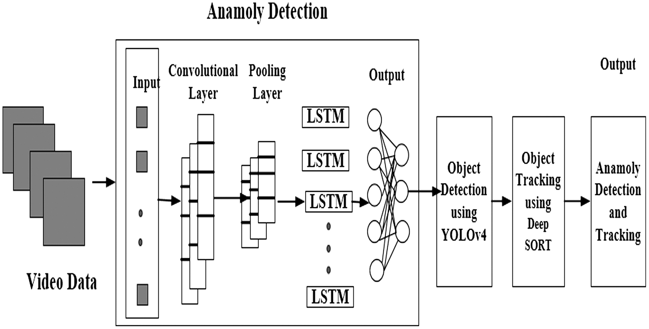 Fig. 1. Overall architecture of the proposed model.
A.PREPROCESSING OF DATA
Resizing is essential for optimizing data in computer vision and video processing, thereby standardizing and normalizing the data frames. In addition to lowering its computational complexity, resizing the frames to a lower resolution speeds up model training. Resized and low-resolution frames use less memory, making its storage and retrieval more fault-tolerant and robust.
B.CNN-LSTM FOR ANOMALY CLASSIFICATION
The input data is maintained at a constant size of 224×224×3. Rectified linear unit (ReLU) is used as a function for activation in the CNN model where 4096 nodes are utilized in the activating function. The input layer is defined with dimensions of (1, 150, 150, 3), indicating that it expects the input data of shape (time steps, width, height, and channels). The first set consists of Conv2D layers and MaxPooling2D layers. These layers reduce the spatial dimensions and extract features from each frame. It introduces 1,792 trainable parameters. The network space characteristics are preserved in the initial layer of convolutional layers using a 7 × 7 convolution kernel. The subsequent convolution layers are substituted with a 3 × 3 convolution kernel, which extracts intrinsic features to recognize the relevant foreground objects from their surroundings. The second set also includes Conv2D and MaxPooling2D layers. The size of the output feature vectors is reduced by the max pooling process used by CNN, which processes the data, making it suitable for further analysis. This layer contributes to 18,464 trainable parameters. Following the CNN layers is a time-distributed layer, which flattens and reshapes the output from the previous CNN layers, converting it into a one-dimensional (1D) vector for each time step. A CNN has around 1500 nodes, which process the input data to produce the desired outcome.
Backpropagating error from the LSTM across several input images to the CNN model trains the CNN. By combining CNN layers, LSTM layers, and a dense layer as the output, a CNN-LSTM model can be created. The main goal of the CNN-LSTM model is to wrap the entire CNN input model (one layer or more) in a TimeDistributed layer, apply it to each input image, and then send the output of each input image to the LSTM as a single time step. The CNN layers are defined first, followed by a TimeDistributed layer, and finally the LSTM with its output layers. The primary characteristic of the LSTM network is the combination of input, output, and forget gates along with the presence of the memory cells in the concealed layer for intrinsic sequence processing. Initially, this layer is defined with hundred units, which captures temporal dependencies and their respective behavioral patterns within the video sequence by processing the flattened feature vectors from the respective time step. The LSTM network processes the one-dimensional vector generated by the prior CNN layers. The LSTM cell processes the data multiple times, learning about the past and subsequent events before obtaining the resultant vector from the recent memory cell. The LSTM network retains a partial amount of memory as it repeatedly scans the input frames sequentially for anomalous target. This memory is updated with recent information from the current observed frame sequences, and the essential data is stored in the internal memory when a new frame is introduced into the modeling network.
The cell state is the center component of LSTM present throughout the entire network operating cycle. It determines the number of frames processed over a period. The sigmoid function is used as the activation function for each of the three gates in the LSTM model. An output of value of 0 or 1 is determined, representing the level of data filtering. When the value of this variable is 0 the information is not transmitted across it, whereas all transmissions are permitted when its value is 1. Further findings are sent to the next layer and the following self by this layer of LSTM. The result is carried out under the pretext of passing the information to the subsequent self as input information while simultaneously passing the results that are generated from each instance to the subsequent layer of LSTM as training data.
The input gate, forget gate, and output gate are the three gates that make up an LSTM unit. Every memory block that makes up the concatenation LSTM has a memory store. Equations (1)–(6) are considered for determining the outputs () based on the input ( of an LSTM for a single time step. In an LSTM network, three gates, namely the forget () gate, the input () gate, and the output () gate, regulate the flow of information flowing through the sequence chain. The values generated by the forget () gate and input () gate with the value of the cell input activation value () are used for internal calculation of the LSTM and are also used for generating cell state value ( and hidden state value (. The notations and are the inputs acquired from the previous time step. The output state (, cell state (, and the hidden state are generated as an input for the consequent time step. Equations (1), (2), (3), (4), (5), and (6) are used for implementing the memory block of the LSTM, which is comparable to the hidden layer of the RNN:
where , , , , , , , and are the input weights and the recurrent weights, respectively, and , , , and are their respective bias variables. Variables and denote sigmoid for gate activation and tanh for input and output activation. The CNN-LSTM’s architecture is depicted in Fig. 2.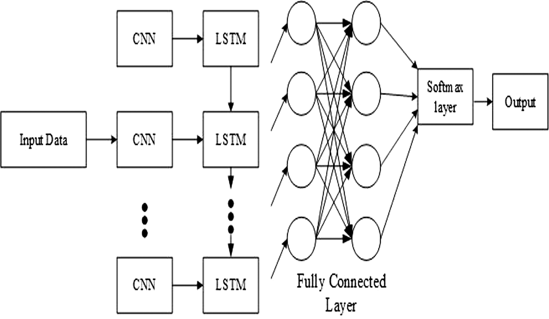 Fig. 2. CNN-LSTM architecture.
An additional component of the noise factor is appended to the LSTM’s first cell states to prevent further loss, which occurs at the initial stage of the LSTM network.
The state of the cell is created with a normal distribution. The bias component of the forget gate is initialized with a binary vector for activation during the training phase. The sigmoid layer of the forget gate regulates the information present in the cell state to avoid the occurrence of the gradient explosions. The LSTM network introduces 16,629,200 trainable parameters, with the output layer consisting of a dense layer of two units with a sigmoid activation function for the primary binary classification. It introduces 202 trainable parameters. The output layer performs binary classification.
C.YOLOv4 FOR ANOMALY DETECTION
YOLOv4 is a single-stage object identification technique applying the regression technique for identifying multiple targets in the same video sequence captured from different perspectives in a rapid and efficient manner. The YOLO Darknet-53 comprises 53 convolutional layers, where each layer is followed by batch normalization applying leaky ReLU as its activation function. The system predicts four coordinates (, , , ) for the bounding boxes. If the coordinates (, ) are the offset coordinates of the top left corner of the bounding box and (, ) and (, ) are the height and the weight of the ground-truth bounding box and predicted bounding box, respectively, then the predictions would be as depicted in equations (7)–(10):
where (, ) represents the center coordinates of the predicted box. and are sigmoid functions of the coordinates and . YOLOv4 switches the prediction function from softmax to autonomous logical classifiers to address the multi-label categorization issue. It also deals with the upsampling and fusion technique of the Feature Pyramid Network (FPN), thereby improving the detection accuracy of the tiny objects. It independently identifies three scaled fused characteristic maps. This architecture also adapts to any gradient issues, increasing its resilience. Figure 3 gives the pictorial representation of the bounding boxes with dimension priors and location prediction.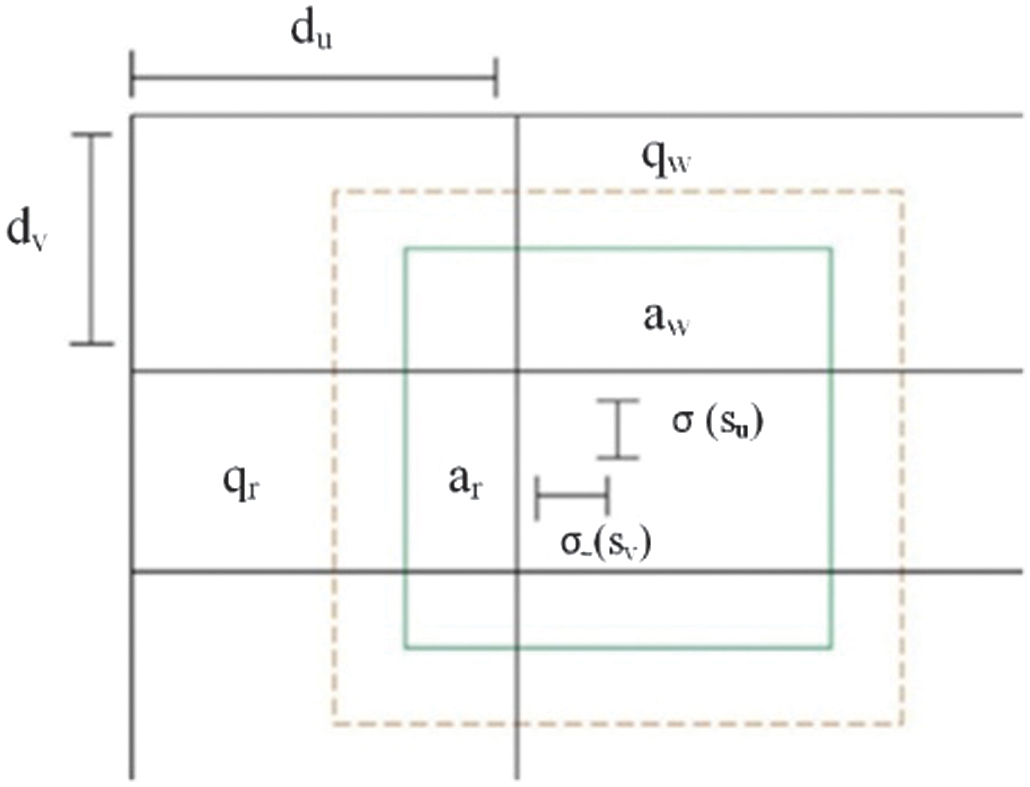 Fig. 3. Bounding boxes with dimension priors and location prediction.
The information of the location of all the identified targets is condensed into an eight-dimensional matrix. This matrix is used to retrieve and plot the current state of the target with the computed bounding box. The eight-dimensional matrix of the trajectory generated by YOLOv4 represents the state of the trajectory’s position at a specific point. The matrix is given by equation (11):
where (, ) represents the center of the bounding box, () is the aspect ratio, and () is the height of the image. Variables () represent their respective velocities.Algorithm 1: Yolov4s with Greedy NMS
| Step 1: Establish a value for both IoU_Threshold and Confidence_Threshold. |
| Step 2: The second step is to arrange the bounding boxes according to decreasing confidence. |
| Step 3: The third step is to eliminate boxes with a confidence less than the confidence threshold. |
| Step 4: Iterate through each of the remaining boxes, beginning with the most confident box. |
| Step 5: Determine the current box’s IoU by comparing it to all of the other boxes in the same class. |
| Step 6: Remove the box with a lower confidence from the list of boxes if the IoU of the two boxes are more than the IoU_Threshold. |
| Step 7: Repeat this operation until all the boxes are processed. |
The first step in the (non-maximal suppression (NMS) process involves sorting the bounding boxes in a decreasing order of confidences. Next, a confidence threshold is defined, which removes any box if it has a confidence that falls below this threshold. Next, a threshold in terms of IoU is defined, which removes boxes with the possibility of having a small overlap. If the boxes share a good overlap, they probably represent the same class. To ensure each object will have only one box, the box with the lower confidence score will be eliminated. Repeat the procedure over all of the sorted boxes till a single bounding box remains having a confidence score higher than the threshold value.
D.MODIFIED DEEPSORT FOR ANOMALY TRACKING
In such tracking algorithms, both motion and appearance descriptors are combined in Deep SORT’s improved association metric. The tracking algorithm DeepSORT is characterized by its ability to track the target not only by their motion and velocity but also by their appearance. Cosine distance aids the model in recovering identities when motion estimation fails and there is prolonged occlusion.
The objective of the DeepSORT tracking algorithm is to track the movements of the target anomalies after assigning a unique identification label for each anomaly. YOLOv4 locates and detects the anomalies, and the DeepSORT tracking technique maintains the tracking consistency even in cluttered environments and minimizes the frequency of ID shifts, enhancing the overall performance of the multi-anomaly tracking. The position of the detected target anomaly in each consecutive frame is predicted, and its current position is updated along its trajectories. The anomalies detected by the eight-dimensional matrix representation of the trajectory by YOLOv4 pass the detections from the current frame to the concurrent frame. The predicted position in the next frame is estimated by the Kalman filter. Equations (12) to (16) define the estimation and correlative operations of the Kalman filter.
Time Update (Predict):
Measurement Update (Correct):
where represents the system state at duration j, represents the future estimation of the state at procedure j, represents the initial forecast of the state at step j, represents the anticipated outcome from the previous state, represents the real-world measurement of u at duration j, represents the previous estimated error covariance, is the predictive measurement, denotes the Kalman gain, R is the noiseless connection that exists between the current state vector and the measurements vector, represents the error covariance, H denotes noise correlation, and the procedure noise covariance is denoted by P.Once the location of the target is estimated in the successive sequential frames, an IoU metric-based cost matrix is created. It is used to calculate the spatial distance between the current detection and the projected bounding boxes of the current tracks. The updated bounding box tracked from the Kalman filter is matched with the current predictions by applying the squared Mahalanobis distance considering the uncertainty of Kalman estimates. In order to maximize this association, the Hungarian algorithm with a matching cascade strategy is considered, where the position of the target is adjusted based on the current trajectory. The tracking matrix is represented by a ‘removal’ as well as a ‘confirmed’ state to filter out incompatible or mismatching predictions. It also improves the tracking accuracy of DeepSORT by integrating a deep appearance descriptor. This feature vector incorporates both the motion and visual aspects of the object which is essential for robust association. The analysis determines the Mahalanobis distance between the location estimated by the Kalman filter and the actual location of the captured frame identified by YOLOv4. Equation (17) provides the mathematical equation:
where is the target’s expected location as determined by the tracker, is the exact location of the recognition structure, and is the coefficient of covariance between the point of detection location and the tracking device position. By applying a pretrained CNN network to extract appearance characteristics, the study performs the same calculation as in Equation (18) to determine the minimal cosine distance between the projected track and the trajectory:The cosine distance incorporates the appearance descriptor which recovers the target’s identification for a target that has been obscured for a considerable amount of time effectively. Equation (19) determines the selection of the predicted bounding box with minimal distance between the predicted and the actual bounding box position of the target:
The cost matrix incorporates both the position and appearance measures through the appropriate cascading condition. By comparing the locations (coordinates) of these two bounding boxes, the measurement is calculated. The evaluation of proximity between the predicted and the actual bounding box depends on measuring its distance known as the Euclidean distance. The expected box’s distance from the preceding box is measured in Euclidean distance. Euclidean distance needs to be minimum than a determined threshold value for better results. When the anomaly target is obscured for a long duration, the target’s tracking trajectory is disrupted, and an alternative path is created, hence giving rise to the issue of frequent ID switching. The Deep SORT algorithm exploits a matching cascade strategy to minimize the frequency of ID switching by combining the target’s motion data with its visual data along with its depth. Anomalies are tracked even for longer durations over consecutive frames, enhancing the resilience and the fault-tolerant nature of the algorithm. Computational processing of the technique increases since storing the relevant path information of the anomaly and updating it across the consecutive frames of the video sequence amounts to time complexity. Following is the step-by-step algorithm for determining accurate results based on the Hungarian algorithm between the predicted and actual distance.
Algorithm 2: Modified Deep Sort
| Step 1: Collect the Database UCSD Ped2 |
| Step 2: Initialize YOLOv4 which is the object detection model |
| Step 3: Apply the Kalman filter for motion estimation |
| Step 4: Initialize the appearance feature extractor |
| Step 5: Initialize the DeepSORT tracker with parameters |
| #Object detection |
| # Detect objects in the current frame |
| #Extract appearance features |
| # Kalman filter prediction |
| for track in active_tracks: |
| for detection in detections: |
| ) |
| for track, detection in matched_tracks: |
| for detection in unmatched_detections: |
| for track in active_tracks: |
| return active_tracks |
The suggested work comes up with an optimized DeepSORT tracking algorithm to improve object tracking performance in dense, cluttered scenes. In contrast to the original DeepSORT, which employs the traditional motion (Kalman filter) and appearance (embedding vector), the modified version has some optimizations. These are as follows:
- •Enhanced appearance feature descriptors learned to separate visually confusable objects in dense environments.
- •Use of both cosine similarity and Mahalanobis distance for more reliable association measures.
- •Adaptive reinitialization logic for reassigning IDs for the reappearance of the objects under occlusion.
- •Threshold adjusting and cascading mechanisms to minimize ID switching, maximizing identity preservation with time.
Change in the following parameters has been applied, portraying its impact on its performance. Specific parameter-level changes that significantly improved performance include:
- •Cosine Distance Threshold: Dropped from the default of 0.6 to 0.45, which caused the tracker to be more discerning in linking new detections with existing tracks. This served to reduce false re-identifications in congested scenes.
- •Appearance Embedding Dimension increased from 128-D to 256-D for finer distinction among objects that look similar (e.g. individuals dressed in similar attire).
- •Matching Cascade Depth: It has been tweaked so that it favors newer confirmed tracks yet retaining older stable ones which is vital for brief occlusion.
These modifications brought better tracking accuracy (97.5%), less ID switches, and better robustness under recurrent occlusions, as shown in dense test situations like multi-anomaly detection on UCSD Ped2. Comparison with the original Deep Sort is shown in Table I.
Table I. Comparison with original Deep SORT
| Feature | Original DeepSORT | Modified DeepSORT (proposed) |
|---|---|---|
| Appearance embedding | 128-D (standard) | 256-D (enhanced descriptor) |
| Association metric | Mahalanobis distance | Mahalanobis + Cosine + IoU fusion |
| Cosine distance threshold | 0.6 | 0.45 (stricter matching) |
| ID re-initialization strategy | Basic logic | Improved recovery with embedding memory |
| Occlusion handling | Limited | Robust, persistent identity tracking |
| Tracking accuracy | ∼95% | 97.5% |
| MAE (multi-target) | 0.354 | 0.32453 |
| Predicted | |||
|---|---|---|---|
| Anomaly | Normal | ||
| Ground truth | Anomaly | ||
| Normal | |||
The modified DeepSORT overcomes the limitations of the original method in high-density and occlusion-vulnerable scenarios by refining association thresholds, augmenting appearance features, and optimizing trajectory continuity reasoning. All these adjustments result in substantially enhanced multi-object tracking performance, which allows for more reliable and coherent anomaly tracking in practical surveillance applications.
V.DATASET
The benchmark dataset of UCSD (Ped2)http://www.svcl.ucsd.edu/projects/anomaly/dataset.html [32] is considered for evaluating and assessing the performance of the proposed approach. This dataset contains frame sequences captured by the stationary cameras positioned overlooking the pedestrian walkways. It includes the admission of pedestrians as well as non-pedestrians’ entities like a truck, skateboard, bicycle, or vehicle in the pedestrian walkways in its university campus. The dataset comprises 16 video clips for training and 12 for testing. Each frame within these clips is annotated with a binary label that specifies whether an anomaly occurs at that particular moment. The pixels are tagged with a 1 for the anomaly and 0 for normal for every frame in each video along with their ground-truth values. The UCSD Ped2 dataset comprises 24 videos from which 12 sequences are anomalous and the other 12 are of normal sequence.
VI.RESULTS AND DISCUSSION
The proposed anomaly detection strategy in crowded circumstances is an integrated methodology that effectively integrates the deep learning techniques of classification, detection, and tracking in a chronological order for accurate and efficient identification of aberrant behavior. The proposed model analyzes and experiments on the benchmark dataset of UCSD (Ped2). The model is run in Python version 3.10.12 with TensorFlow framework version 2.13.0-rc0. OpenCV version 4.7.0 is applied along with NumPy and SciPy of versions 1.25.2 and 1.9.1, respectively.
A.ANOMALY CLASSIFICATION
The snapshots of the images serve as a visual representation of the dataset UCSD Ped2. The data sample in Fig. 4 contains (a) a normal image that represents the baseline of the dataset, (b) the entry of the truck into the frame, and (c) the entry of a truck and a cycle in the same video frame.
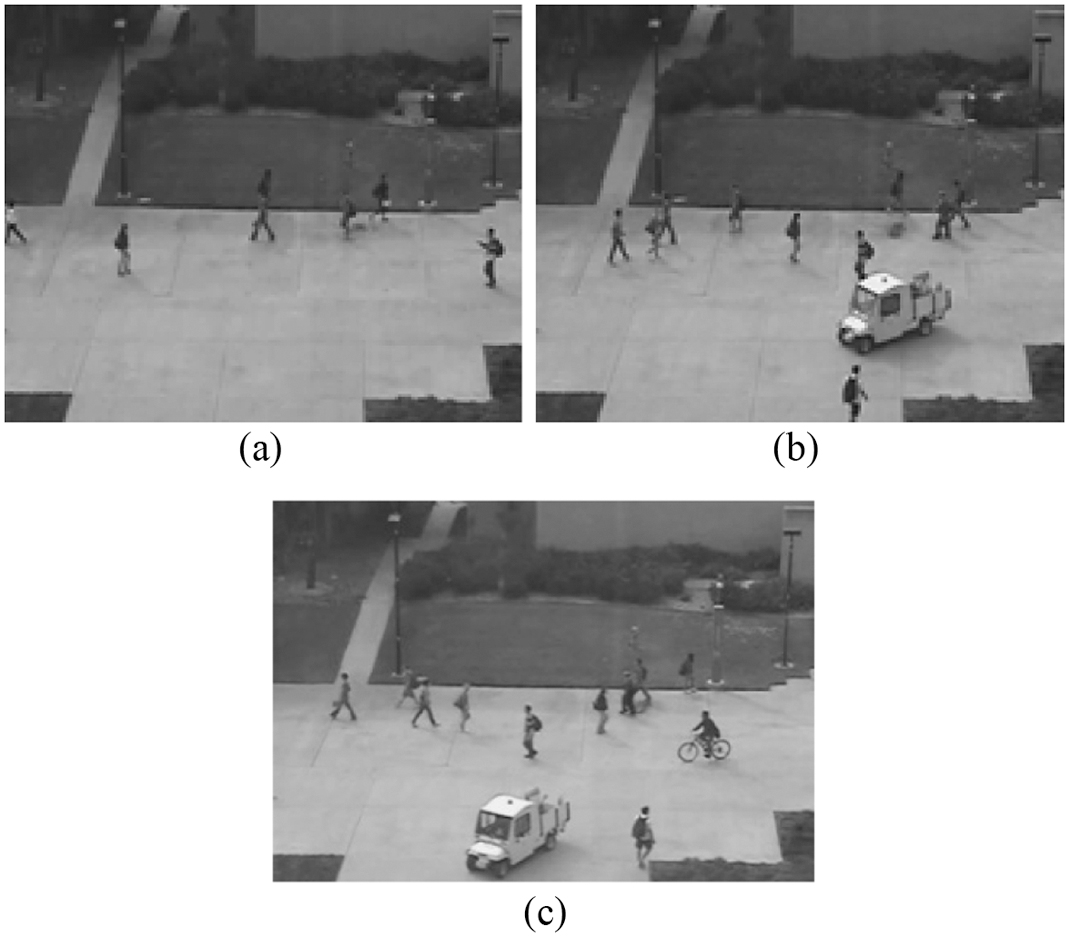
Figure 5 illustrates the labeled anomaly frames after CNN-LSTM classification. In Fig. 5(a) the frame is classified as “normal” in the frame where no abnormalities are found. Figure 5(b) and (c) depicts flagging the scene as an “anomaly” with the entry of the moving truck and a cycle into the video frame in the pedestrian walkways.
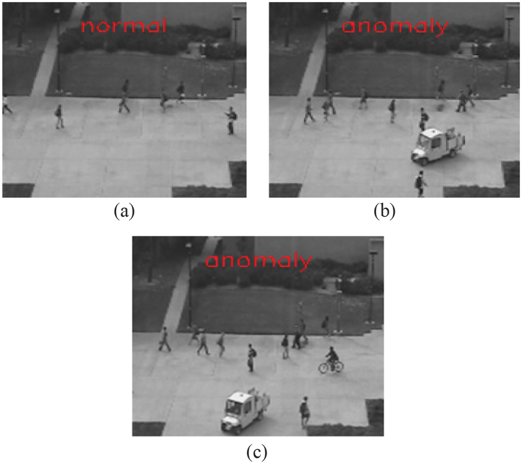
Figure 6 gives an illustration for detecting and tracking the anomalies in the consecutive video frames of the UCSD Ped2 dataset. Figure 6(b) labels the video frame as “anomaly” after CNN-LSTM classification. Figure 6(c) depicts single-anomaly detection and localization by the YOLOv4 detection algorithm with a bounding box. Figure 6(d) illustrates the Deep SORT tracking method of the detected single anomaly keeping track of the anomaly truck in the video snippet.
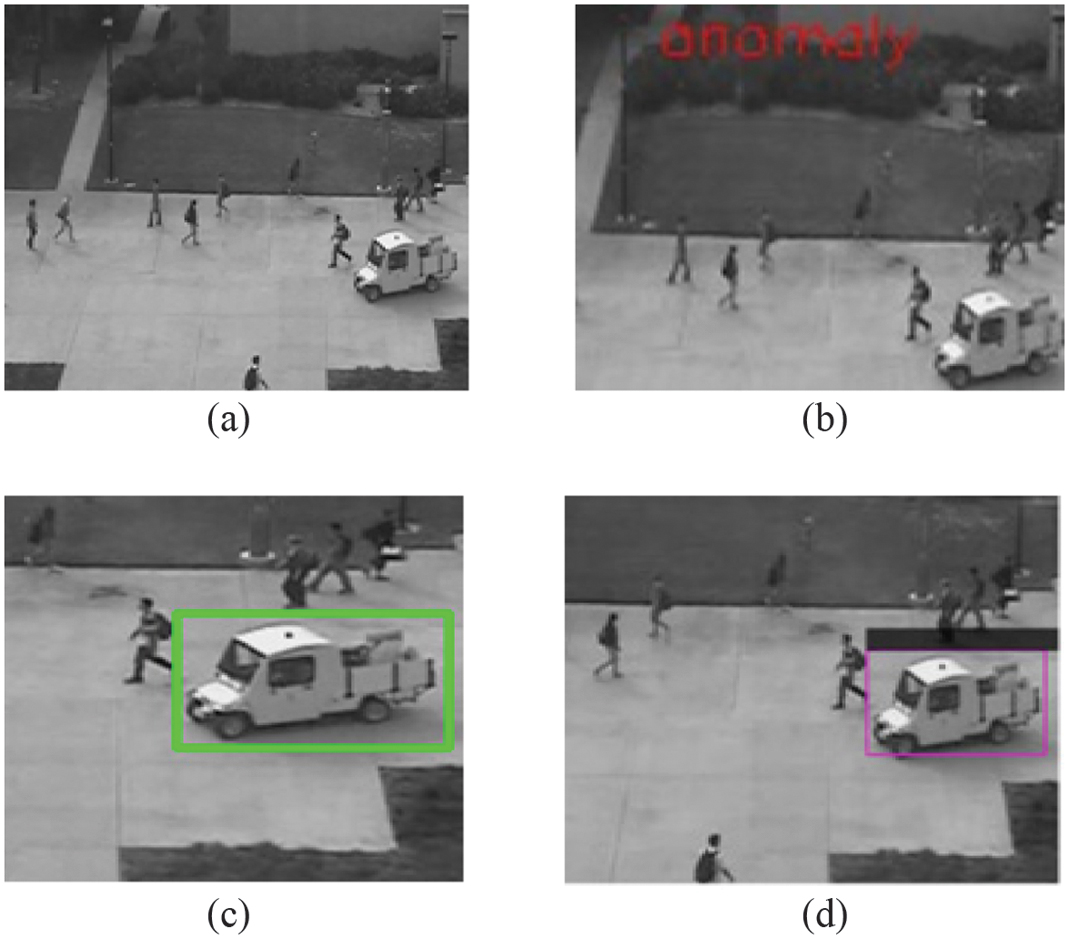 Fig. 6. Single-target anomaly classification, detection, and tracking: (a) normal, (b) anomaly, (c) detection, and (d) tracking.
Figure 7 depicts a complex system of multi-anomalies in the same video sequence. The frame in Fig. 7(b) depicts and labels the frame as “anomaly” after CNN-LSTM classification due to the entry of both a truck and a cycle in the same pedestrian walkway. The Yolov4 detection algorithm detects and localizes the moving truck and the cycle simultaneously with the bounding boxes in the frame of Fig. 7(c). In Fig. 7(d), the Deep SORT tracking algorithm tracks the detected anomalies contained in the video sequence.
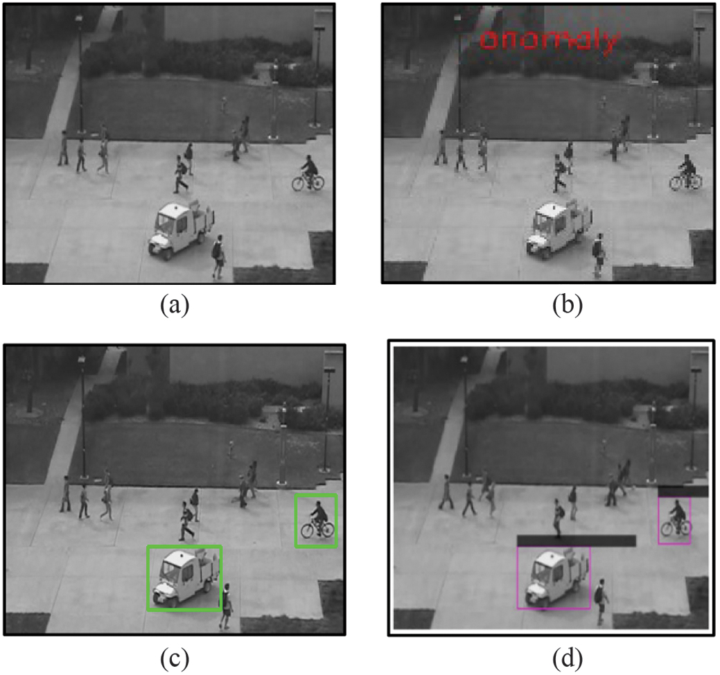 Fig. 7. Multi-target classification, detection, and tracking: (a) normal, (b) anomaly, (c) detection, and (d) tracking.
1)PERFORMANCE METRICS
The classification metrics evaluate the performance of the proposed model. Metrics used are precision, recall, F1-score, and accuracy. These metrics are computed based on the probability values of True Positive (), True Negative (), False Positive (), and False Negative () as depicted in Table II. The True Positive signifies the correct number of anomalies predicted by the model. True Negative signifies the correct number of normal frames predicted by the model. False Positive (Type I error) signifies the incorrect number of normal frames predicted by the model. False Negative (Type II error) signifies the incorrect number of anomalies predicted by the model.
Precision. Precision is the ratio of true positives and total positives predicted. Precision corresponds to identifying the proportion of identified anomalies as true anomalies in the given occurrences. This metric focuses on incorrectly labeling anomaly frames as normal which is a Type I error (). It is given by equation (20):
Recall. Recall is the ratio of true positives to all the positives in ground truth. It identifies the proportion of true anomalies. Recall defines the sensitivity of the anomaly detection. This metric focuses on incorrectly labeling normal frames as anomalies which is a Type II error (). This metric is expressed by equation (21):
F1_score. F1-score is () the harmonic mean of precision and recall which considers false positives and false negatives. It is characterized by equation (22):
Accuracy. Accuracy measures the proportion of correct predictions. It determines correctly predicted instances to the total instances in the dataset. It is given by equation (23):
AUROC. AUROC represents the Area Under the Receiver Operating Characteristic curve. The AUROC curve measures the model’s ability to distinguish between positive and negative classes. It plots the graph with True Positive Rate () against the False Positive Rate (). The equations are shown in equation (24):
The ROC curve graph in Fig. 8 exhibits performance for single- and multiple-anomaly classification. The ROC curve shows the True Positive Rate (Sensitivity) compared to the False Positive Rate (1-Specificity) at observed threshold levels for identifying abnormalities. The plotted graph at each threshold value demonstrates that the model can distinguish between normal and anomalous instances for single- and multi-target anomalies. It can be observed that the model can distinguish the anomalies from normal in the video frames while retaining a low false positive rate.
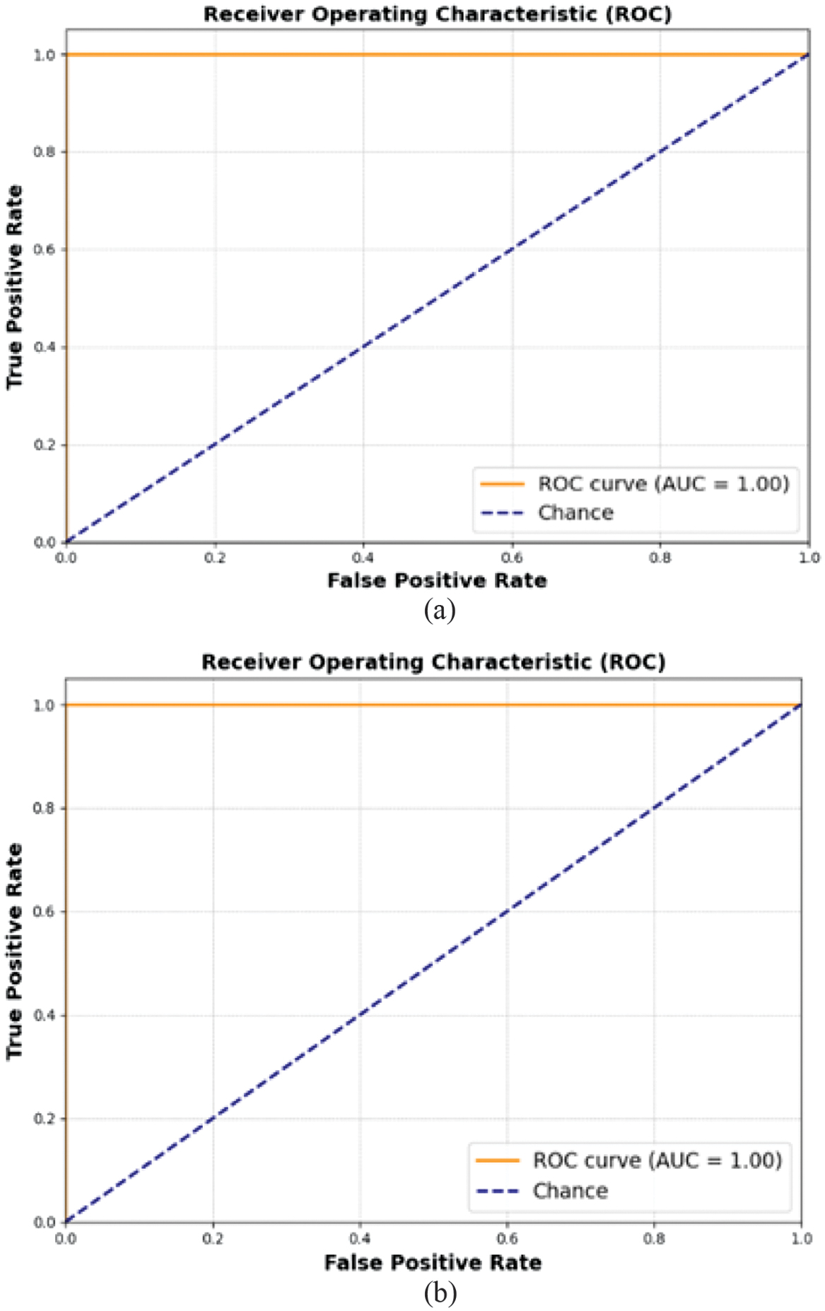 Fig. 8. AUROC curve: (a) single-target anomaly and (b) multi-target anomaly.
The training and validation accuracy for a CNN-LSTM-based single-object anomaly classification model is shown in Figure 9(a). The initial values of the training accuracy and validation accuracy are 0.58 and 0.5, respectively, in the first epoch, attaining numerical values of 0.97 and 0.99 in the sixth epoch. From the graph it can be deduced that the CNN-LSTM model effectively learns from the training data identifying the anomalies. Figure 9(b) illustrates multi-anomaly classification where the values of training and validation accuracy have comparatively lower values at inception. Initially, the training accuracy gradually rises with validation accuracy remaining at 0.5. The training accuracy approaches 0.97 by the last epoch, but the validation accuracy remains at 0.99 denoting potential overfitting. To improve its efficiency in crowded settings with numerous objects, additional optimization techniques can be incorporated.
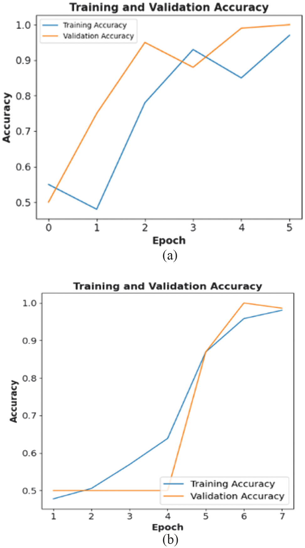 Fig. 9. Training and validation accuracy: (a) single-target anomaly and (b) multi-target anomaly.
Figure 10(a) and (b) depicts the training and validation loss of a CNN-LSTM classification for a single- and multi-anomaly scenario. The training loss begins at a value of 0.97 with the validation loss at 0.71 during the first epoch and gradually decreases with an increase in each epoch. Hence, the loss values are minimized with the implementation of the CNN-LSTM classification model yielding more effective and reliable classification of anomalies. In the case of multi-anomaly classification, the training loss is fairly high in the first epoch with a value of 0.99 with the validation loss being equal to 0.69. After the fifth epoch, the training loss falls to the value of 0.10 with the validation loss being close to 0.11. The validation loss remains slightly higher than the training loss in Fig. 10(b) during epoch 3. The training and validation loss curves reveal steady improvement in both cases, but the multi-anomaly scenario still exhibits slightly higher validation loss. Overfitting can be mitigated by incorporating optimization techniques such as dropout and early stopping. Overall, the CNN-LSTM model requires additional fine-tuning to handle more complex multi-anomaly scenarios effectively.
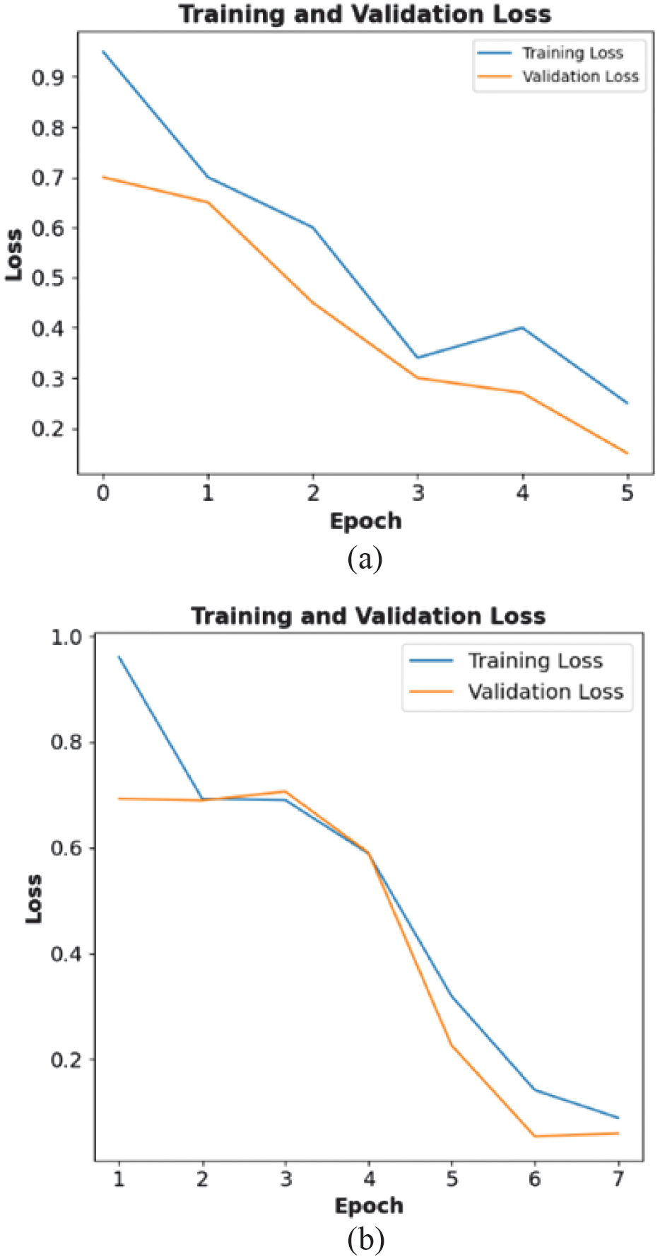 Fig. 10. Training and validation loss: (a) single-target anomaly and (b) multi-target anomaly.
Figure 11(a) and (b) portray the performance metrics for the single-anomaly and multi-anomaly CNN-LSTM classification model. The metrics evaluate and assess the model. From the plotted charts, it can be observed that the metrics of precision, recall, and F1_score are observed to be of value 99% and accuracy with a value of 99.8% which speaks of credible performance in the performance of the CNN-LSTM model.
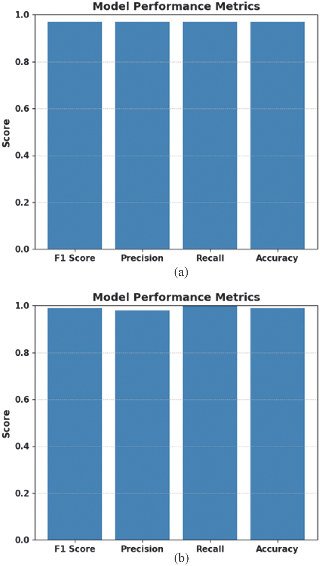 Fig. 11. CNN-LSTM performance metrics: (a) single-target anomaly and (b) multi-target anomaly.
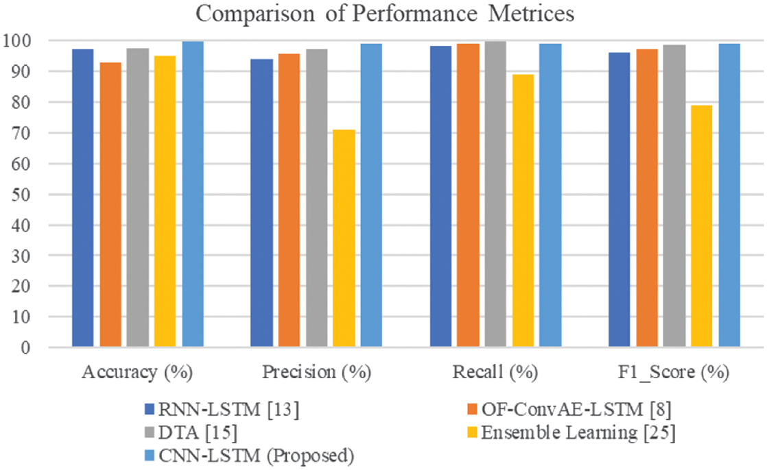
Table III identifies a better performance of the developed CNN-LSTM-based anomaly classification model, with the highest accuracy (99.8%) and balanced precision, recall, and F1-score (all equal to 99%). This is due to the combination of CNN to extract rich spatial features from frames of the video and LSTM networks to capture temporal dependencies from frame sequences. On the other hand, RNN-LSTM [13] is based purely on temporal modeling and does not have fine-grained spatial extraction, making its classification score (97.13%) limited. OF-ConvAE-LSTM [8] has used OF for motion signals but is affected by background noise, which affects accuracy (92.9%). Bi-LSTM [25], although it has bidirectional temporal learning capability, has low precision (71%), which means high false positive rates with a lack of proper spatial feature encoding. The introduced CNN-LSTM bridges the above disparity successfully by integrating the spatial and temporal learning, making the model stronger and more accurate in classifying anomalies in crowded scenes.
Table III. Comparison of performance evaluation
| Techniques | Accuracy (%) | Precision (%) | Recall (%) | F1_Score (%) |
|---|---|---|---|---|
| RNN-LSTM [ | 97.13 | 94.12 | 98.23 | 96.1 |
| OF-ConvAE-LSTM [ | 92.9 | 95.8 | 98.9 | 97.3 |
| DTA [ | 97.5 | 97.3 | 99.8 | 98.5 |
| Ensemble Learning [ | 95.1 | 71 | 89 | 78.9 |
| CNN-LSTM (proposed) | 99.8 | 99 | 99 | 99 |
Figure 12 portrays its comparative analysis of the methods of RNN-LSTM [13], OF-ConvAE-LSTM [8], DTA [15], and Ensemble Learning [25] with the proposed CNN-LSTM approach for anomaly detection and classification. The proposed CNN-LSTM method outperforms the mentioned techniques based on the performance of the model with an accuracy of 99.8% and precision, recall, and F1-score of 99%. Hence, the ability to discover and classify the existing anomalies in the video frames by the proposed model is done in a proficient manner, thereby minimizing the number of false positives and false negatives in the given dataset.
B.ANOMALY DETECTION AND TRACKING
1)CONFIDENCE SCORE AND IOU
YOLO version 4 object detection technique uses a post-processing technique of NMS which iteratively chooses the detected bounding box of the target with the highest confidence score from the detected score ratings. Greedy NMS selects the predicted bounding box of the highest degree of confidence score among the list of bounding boxes closer to the ground truth. It eliminates the duplicate bounding box detections and selects the most relevant of the highest confidence score bounding boxes that correspond to the detected objects. Greedy NMS removes unnecessary bounding boxes by holding onto the most confident detections, guaranteeing a clearer and cohesive output.
It minimizes the amount of redundant and overlapping predictions, which improves post-processing, enabling it to do more precise downstream tasks with ease, like tracking or classification. The IoU metric is the ratio of the overlap area between the predicted and the ground-truth bounding boxes to their combined area. The IoU is computed as in equation (25):
An untracked item is identified and given a new tracking identification. Tracking implicitly restarts with the new identity if the item reappears, effectively overcoming the issue of re-identification. This work uses a systematic approach for tracking that includes identifying the target bounding box and the detected bounding boxes evaluating a cost matrix. The distances between ground truth and predicted bounding boxes from existing targets apply the Hungarian algorithm to solve the assignment problem optimally. This minimizes the computational cost, hence increasing the rate of detection.
Figure 13(a) and (b) depict the loss function of the YOLOv4 for single- and multi-anomaly detection in the UCSD Ped2 dataset. The loss function gives critical feedback on the minimal loss incurred between the predicted and the actual anomalies during the detection process. The current average loss for detecting a single anomaly is 0.6812 for the iteration count of 900 and 0.2834 for the detection of multi-anomaly for the iteration count of 2800. It is evident from Figure 13(a) and (b) that the detection model for a single anomaly performs better at tracking individual objects inside video frames as the loss appears to decrease with an increase in iteration.
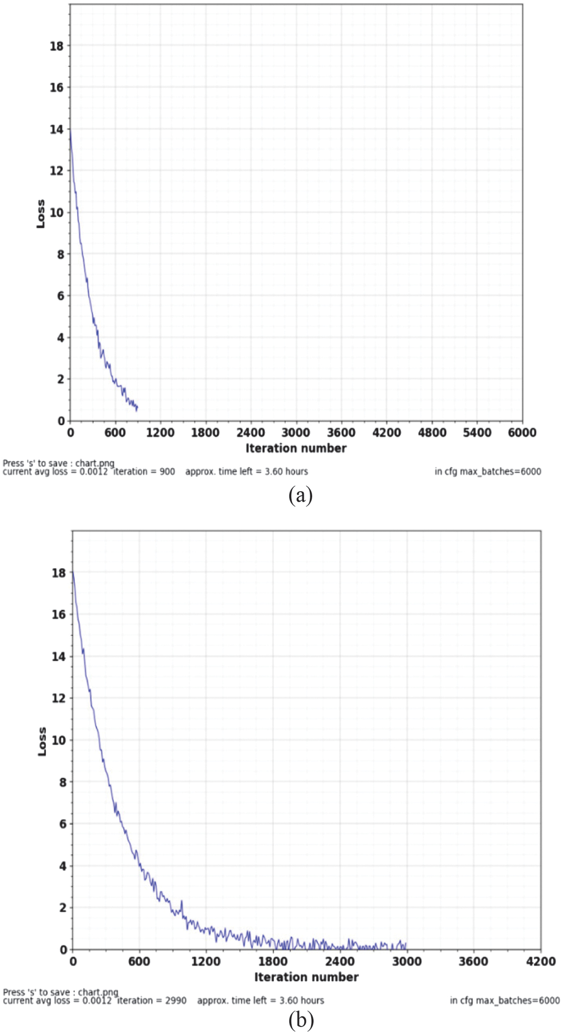 Fig. 13. YOLOv4 loss function for (a) single-target anomaly and (b) multi-target anomaly.
Table IV portrays the proposed YOLOv4 model exhibiting a better anomaly detection accuracy with an IoU of 89.6% at 22 frames per second depicting highly precise object localization. It also has a detection loss of only 0.28 in multi-target detection, illustrating effective training convergence. Precision attained is 99.0%, illustrating higher precision in comparison to other YOLOv4-based methods. For instance, CNN-YOLOv4 of reference article [23] experienced a greater loss (0.35) with lesser precision (89%), and YOLOv4 with IFCM of Gao et al. (2023) [24] achieved lower IoU (84%) and 87.1% in precision. Yao et al. (2021) [30] implements SPP attaining a comparatively higher precision of 94.09% at 44 FPS not mentioning loss or IoU. The suggested YOLOv4 retains real-time performance at ∼22 FPS, which optimizes accuracy and speed harmoniously. In general, the suggested methodology surpasses current works with respect to the detection and the localization quality for abnormality detection in video frames.
Table IV. Comparison of YOLOV4 in anomaly detection
| Method | IoU | Detection | Precision (%) | FPS |
|---|---|---|---|---|
| YOLOv4 with Greedy NMS (proposed) | 89.6 | 0.28 (multi-target) | 99.0 | ∼22 |
| CNN-YOLOv4 [ | - | 0.35 | 89 | - |
| YOLOv4 with IFCM [ | 84 | - | 87.1 | - |
| YOLOv4 [ | - | - | 94.09% | 44 |
2)MEAN SQUARED ERROR (MSE)
Mean squared error () measures the average squared difference between the target value and the predicted value of the model in the dataset. It is characterized by equation (26):
where m is the number of data, is the ground-truth value, and is the predicted value.3)MEAN ABSOLUTE ERROR (MAE)
Mean absolute error () is the average of the difference between the ground truth and the predicted values. It is characterized by equation (27):
where m is the number of data, is the ground truth, and is the predicted values.Figure 14 exhibits the visualization of MSE and MAE with respect to the frame sequence for single-anomaly detection using YOLOv4-Deep SORT. It is interpreted that the MAE is 0 at frame numbers 5, 7, and 9 and approximately 5 for frames 6 and 8. However, at the same point of time, the value of MSE is 0 at frame numbers 5, 7, and 9 and reaches the value of 43 twice for frame numbers 6 and 8, indicating a considerable disparity between projected and actual values. The MSE and MAE reduce to 0 in frame 9 and continue to have the same value for the next 25 frames with a small spike in the twentieth frame. This indicates the predicted value of the model lies in close proximity to the ground truth after 20 frames.
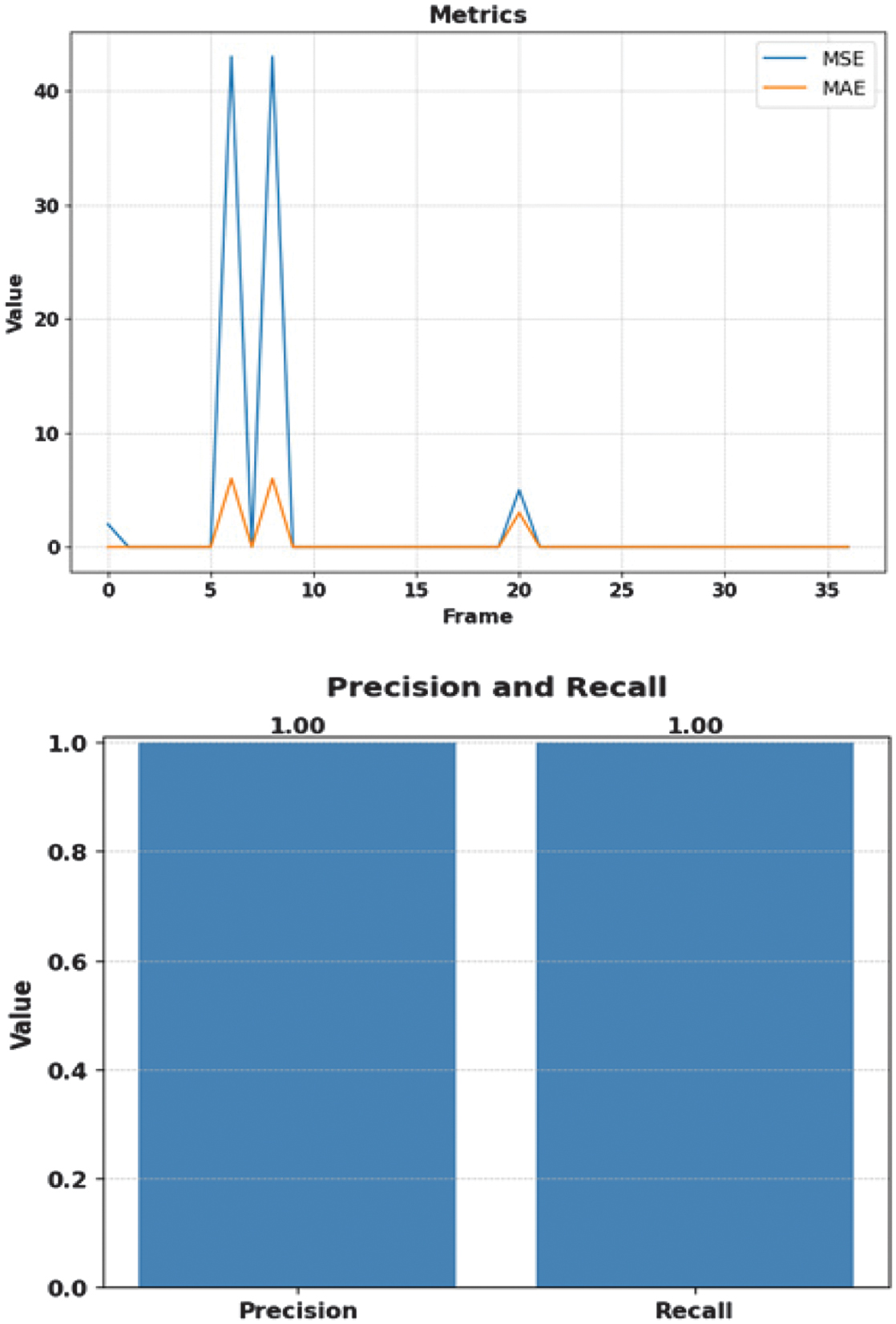 Fig. 14. MSE and MAE of single-target anomaly.
The performance of the multi-anomaly detection with YOLOv4-Deep SORT at different anomaly thresholds is depicted in Figure 15. The model has significantly high MSE and MAE values for frame numbers 5 and 10 due to the occurrence of a greater number of false positives and missed abnormalities. The values of MSE and MAE spike up for frame number 20, in which the model was unable to detect the anomalies correctly in the initial stage. Nevertheless, the values of MSE and MAE have been observed to be null for frame numbers 10, 15, 25, 30, and 35, signifying correct predictions.
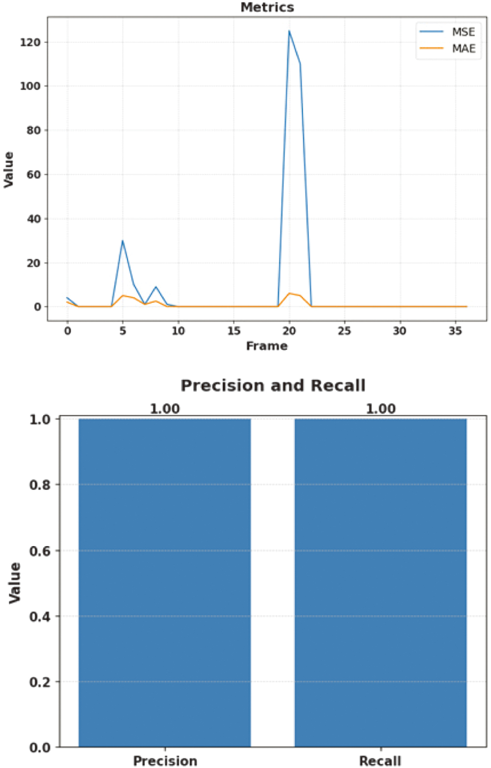 Fig. 15. MSE and MAE of multi-target anomaly.
Table V shows the MSE and the MAE value for single-anomaly detection. They have been observed as 2.71323 and 0.43382, respectively, for the YOLOv4-DeepSORT model. The MSE and the MAE values for multi-anomaly detection have been noted as 2.61232 and 0.32453, respectively. It has been perceived that both single- and multi-anomaly detection approaches have been observed to minimize the squared discrepancies between their predictions and the observed values. However, the YOLOv4-DeepSORT multi-anomaly detection model marginally outperforms the single-anomaly detection in terms of MAE and MSE by 0.10929 and 0.10091, respectively.
Table V. MAE and MSE of single-target and multi-target anomaly detection and tracking
| Anomaly | MSE | MAE |
|---|---|---|
| Single-target anomaly detection and tracking | 2.71323 | 0.43382 |
| Multi-target anomaly detection and tracking | 2.61232 | 0.32453 |
Figure 16 illustrates the visualization of the performance of the YOLOv4 detection with the Deep SORT tracking technique in crowd anomaly detection. The above graphical representation offers insights into the ability to locate and detect multi-anomalies in each video frame sequence with minor deviations. The proposed model can detect and track anomalies, hence monitoring and maintaining vigilance and peace in every society. The result displays the ability of the proposed model to detect and track single and multiple anomalies like trucks and bicycles entering a pedestrian area. Performance is measured which returns better results with 99% in accuracy and 99.8% in precision.
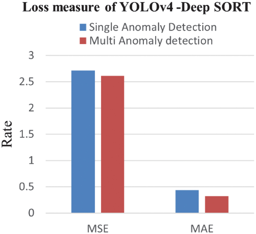 Fig. 16. Loss function of YOLOv4-Deep SORT.
Table VI compares the proposed Deep SORT tracking technique with existing techniques. It posts an impressive tracking accuracy of 97.5% in comparison to CNN-YOLOv5 DeepSORT [26] which achieves only 95%. This reflects an improved uniformity in tracking anomalies of trucks and bicycles in the video frame sequences. The suggested method contains an MAE of 0.43382 for single-target and 0.32453 for multi-target cases, comparable to the MAE of CNN-YOLOv5_DeepSORT and CM Graph-DeepSORT, which is 0.38 and 0.354, respectively. The MSE for the proposed method is 2.71323 (single-target) and 2.61232 (multi-target), indicating slightly greater variance than other methods such as CNN-YOLOV5-DeepSORT, which has an MSE value of 0.22 and the value of CM Graph-DeepSORT technique for multi-target is 0.258. Even with the increased MSE, the suggested model observes lower ID switches, hence strengthening the re-identification of the target under occlusion-intensive conditions leading to a reliable and improved tracking approach in densely populated environments.
Table VI. Comparison of DeepSORT in anomaly tracking
| Method | Tracking accuracy (%) | MAE (mean absolute error) | MSE (mean squared error) |
|---|---|---|---|
| Modified DeepSORT (proposed) | 97.5 | 0.43382 (single target) | 2.71323 (single target) |
| CNN_YOLOv5 DeepSORT [ | 95 | 0.38 | 0.22 |
| CM Graph-DeepSORT [ | - | 0.354 (multi-target) | 0.258( multi-target |
The proposed framework integrates CNN-LSTM for anomaly classification, YOLOv4 for object detection, and Deep SORT for tracking, resulting in a layered pipeline with distinct computational footprints. The CNN-LSTM module introduces temporal modeling, with a time complexity of ), where T is the number of frames per sequence, d is the frame dimension, and k is the number of convolution filters. LSTM introduces additional sequential overhead with recurrent dependencies, scaling linearly with sequential length. Space complexity is dominated by LSTM hidden states and convolutional feature maps, approximately where h is the number of hidden units. The YOLOv4 detection phase exhibits a time complexity of per frame due to multi-scale feature extraction and anchor box regression, where N is the number of bounding box predictions. Deep SORT tracking incurs , time complexity due to pairwise object association using Kalman filtering and Mahalanobis with cosine distance metrics, where m is the number of objects per frame. Space complexity increases with storage of historical appearance embeddings and motion vectors. The integrated model introduces higher complexity, optimized network depth, resized inputs, and Greedy NMS leading to real-time execution at ∼22 FPS with balanced memory usage.
However, the model would face issues in multi-anomaly scenarios, such as overfitting, for which further optimization techniques can be used, such as dropout and early stopping. The model outperforms existing approaches, offering robust anomaly detection and tracking capabilities. The integration of Greedy NMS and IoU in YOLOv4 enhances in evaluating the optimal target bounding box sufficing the efficiency of detection.
The time and space complexity of the proposed method are compared with the respective reference papers as mentioned in Table VII, where it is observed that the proposed method incurs high spatial and temporal complexity due to combined modules.
Hence, the proposed model is optimized using time-distributed layers, adaptive NMS thresholding, and adaptive threshold adjustment for cosine distance.
Table VII. Comparative analysis on time and space complexity
| Method | Time complexity | Space complexity | Real-time performance (FPS) |
|---|---|---|---|
| RNN-LSTM [ | O (T × h) | O (T × h) | ∼15 FPS |
| OF-ConvAE-LSTM [ | O (T × d2) | O (T × d2) | ∼10 FPS |
| YOLOv4-IFCM [ | O (N × d2) | O (N) | ∼30 FPS |
| CNN-YOLOv4 [ | O (N × d2 + T × d2 × k) | O (N + T × h) | ∼18 FPS |
| Proposed model | O (T × d2 × k + N × d2 + m2) | O (T × h + T × d2 + m × D) | ∼22 FPS |
VII.CONCLUSION AND FUTURE WORK
Smart video surveillance has become a necessary paradigm in the field of technology, securing us from unnecessary criminal and violent acts such as robbery, theft, fights, and vandalism. The surveillance systems monitor, detect, and alert the suspicious behavior even in a populated area. Enhanced techniques of object detection and tracking with improved accuracy and reliability in anomaly detection have been observed by leveraging deep learning, and complex computer vision techniques such as CNN-LSTM anomaly classification, YOLOv4-based anomaly detection, and Deep-SORT-based anomaly tracking have been effectively integrated in this study to produce a robust anomaly detection technique designed for populated environments. The proposed method has proven to be remarkably effective in detecting and tracking anomalous behaviors in the UCSD (Ped2) dataset. It becomes imperative to optimize the model’s scalability and real-time performance for city-wise monitoring. The suggested technique also offers insightful information for video surveillance applications by continuously monitoring and flagging the anomalies even in the crowded situations, thereby improving public security and safety issues.
Investigations on more sophisticated detection and tracking techniques which demand high vigilance even in emergency situations are essential in varied aspects of the situation. At present, the deployment of the surveillance systems is the need of the hour to establish a strong basis for more versatile anomaly detection systems with new technological advancements, which can perform well even in congested areas. Hence, early and immediate reporting of the anomalies will alert the crowd, safeguarding the public from any kind of frightful situations making our world a peaceful and violence-free place to live in.