JAIT

I.INTRODUCTION

In the context of global climate change and increasingly severe resource and environmental constraints, green and low-carbon development has become an important strategic direction for enterprise supply chain management. As a key link connecting production, distribution, and consumption, the logistics supply chain has a particularly prominent impact on the environment due to its pollution emission problems, for example, transportation exhaust, manufacturing waste, etc. [1]. According to statistics, the global logistics and transportation industry contribute about 8–10% of carbon emissions, and pollution emissions from the manufacturing stage are one of the main sources of industrial pollution. At the same time, consumers are becoming more aware of environmental protection, and government regulations are becoming increasingly stringent, for example, “dual carbon” targets. This awareness forces companies to optimize their supply chain networks to reduce pollution emissions while meeting capacity constraints, for example, warehousing, transportation capacity [2,3]. Supply chain management involves more process links, which aim to improve enterprise efficiency and productivity through optimization and coordination, and to meet customer demand. Moreover, it contains more contents, such as network design, resource allocation, planning and selection, and so on.

Existing green supply chain research has mostly focused on end-of-pipe management (e.g., recycling) or a single link (e.g., transportation carbon emissions). It pays insufficient attention to collaborative pollution control in the supply-manufacturing chain and lacks a multi-objective optimization method under dynamic capacity constraints. In addition, traditional heuristic algorithms used to solve large-scale green supply chain network (GSCN) problems tend to fall into local optimization. This makes balancing the quality of the solution with computational efficiency difficult. To improve the above problems, this study proposes an intelligent optimization method for green logistics supply chain oriented to pollution emission and capacity constraints. The study constructs a multi-stage GSCN model, focuses on optimizing the supply stage (raw material transportation pollution) and manufacturing stage (production emission), and introduces constraints. The periodic restoration of the marine predators algorithm (PR-MPA) is also proposed to improve the search efficiency. The goal of minimizing total operating costs can be achieved by using a GSCN design solution that satisfies pollution control and capacity constraints simultaneously. This solution provides enterprises with economic and environmental decision support to achieve sustainable development.

The innovation of the research are reflected in two aspects. One approach is to introduce “pollution emission ceilings” and “node capacities” as hard constraints in GSCN. This construction avoids the weight sensitivity problem caused by the traditional “internalization of emission costs” approach. The proposed two-dimensional stage repair-based marine predator algorithm (MPA-SR) incorporates the “path decision operator + greedy freight volume allocation operator” into the MPA’s Levy Brown search framework for the first time. This achieves the efficient repair of discrete and continuous mixed variables. The rest of the study is structured as follows. Section II provides a systematic review of the relevant research on green supply chains and network structures. It summarizes the latest progress in carbon emissions, capacity constraints, and multi-objective optimization. Section III elaborates on the research question and model assumptions. It presents a GSCN mixed-integer programming model that considers pollution emissions and capacity constraints. Finally, it designs a MPA based on phased remediation strategies. Section IV is the results of the proposed method that are verified through case studies and comparative analysis of model performance. Section V is a summary of the entire text and prospects for future improvement directions.

II.LITERATURE REVIEW

Aiming at the green energy-saving logistics location allocation problem, Tirkolaee et al. designed a supply chain network including factories, warehouses, and retailers. The supply chain network problem with the objective of minimum total cost was also solved by gray wolf optimization and particle swarm optimization algorithms. The results indicated that the algorithm could effectively reduce the computation time and provide a solution [4]. Aiming at the siting problem of distribution allocation in GSCN for vaccine response, Goodarzian et al. proposed to design and solve the problem with the help of a multi-objective mathematical model and an improved meta-heuristic algorithm. The results showed that the method exhibited better computational efficiency and convergence, and the evaluation advantage was more obvious under the case data test [5]. Considering the problem of conflicting objectives between logistics distributors and manufacturers, Camacho-Vallejo et al. constructed a dual-objective two-layer planning problem and implemented the planning problem solution to minimize supply chain carbon emissions with the help of tabu search (TS). The results indicated that the algorithm could effectively solve the decision solution and balance the distributor profit and carbon emission [6]. Lotfi et al. proposed constructing a sustainable supply chain with multi-objective planning for designing a closed-loop logistics supply chain network. They solved this problem using Lagrangian relaxation and stationary optimization methods. The results showed that the method could effectively estimate the cost and energy consumption with good applicability [7]. The fluctuation of carbon prices and emission quotas affects low-cost and low-carbon development. Tariffs, FTAs, and the electricity structure of multiple countries are among the factors related to this development. Kotegawa et al. proposed to construct a life cycle material list and embed a total control trading mechanism to achieve low-cost and low-carbon development, and to draw a network using mixed integer programming. The results indicated that increasing carbon prices could reduce emissions more significantly than tightening quotas. This model could provide a quantitative basis for enterprises to design low-carbon global networks in a floating carbon market [8]. On the other hand, Gholipour et al. proposed an intelligent algorithm and reverse logistics design for pomegranate waste to construct a sustainable closed-loop supply chain logistics network. The results showed that the method could effectively reduce the supply chain cost and risk and realize the Pareto problem-solving [9]. Using panel data regression, Wang et al. tested whether intelligent supply chain construction reduced corporate debt financing costs by reducing information asymmetry. They found that, on average, debt costs decreased by about 9 basis points for every one standard deviation increase in intelligence level. The effect doubled in high financing constraint subsamples [10].

It has become a core issue of current research to construct a GSCN that takes into account environmental sustainability and operational feasibility under the premise of guaranteeing economic benefits. Traditional supply chain network design mostly aims at cost minimization or profit maximization, ignoring environmental externalities, leading to excessive resource consumption and pollution [11,12]. In contrast, green supply chains, by integrating environmental constraints (e.g., carbon emission limits, pollution emission standards), are able to reduce negative ecological impacts from the source, while enhancing the long-term competitiveness of enterprises [13]. Among them, Li D introduced the Gaussian variational improved MPA to realize the GSCN problem model solving. The results indicated that the method showed better convergence speed on the test function and could successfully converge to the optimal solution at different scales [14]. Experiments by Li et al. revealed that plasma membranes have the lowest flux attenuation in complex water quality. This finding could help reduce the increase in energy consumption and maintenance costs caused by scaling in reverse osmosis membranes in power plants. They could reduce the frequency of membrane replacement and provide a simple and efficient technical path for water conservation and emission reduction in power plants [15]. Liu et al. designed a multilevel distribution network for e-logistics and proposed to implement iterative prediction and optimization with an artificial neural network (ANN) and a mixed integer linear programming model. The results indicated that the method could effectively reflect the relationship between demand and network design with good prediction accuracy [16]. Yadav incorporated multichannel distribution into the supply chain network design to improve the sustainability as well as flexibility of the supply chain by increasing the objective function to minimize the carbon content as well as supply chain cost. The model had better sustainability, enabled distribution network integration, and had better customer satisfaction [17]. Ehtesham Rasi proposed a multi-objective optimization of a sustainable supply chain network considering economic and environmental factors. Moreover, the optimization of supplier selection and selection of performance indicators was achieved with the help of a mixed integer linear programming model and a genetic algorithm. The results showed that the model could effectively save cost and time and maximize the optimization of system sustainability indicators [18]. Jabarzadeh proposed a sustainability-compliant multi-objective mixed integer linear programming model. This research method could help supply chain managers to develop a fruit sustainable network configuration strategy, which in turn could minimize the cost and economic sustainability in site optimization as well as facility selection [19].

III.GSCN INTELLIGENT OPTIMIZED DESIGN

A.DESIGN OF GSCN OBJECTIVE FUNCTION CONSIDERING POLLUTION EMISSION AND CAPACITY CONSTRAINTS

The main goal of supply chain network design is to reduce the total cost of ownership while satisfying customer demand and to improve the efficiency of the organization. However, its excessive focus on cost-effectiveness has caused it to ignore the environmental impacts and resource efficiency generated during the design phase [20]. GSCN design has become a key strategy for enterprises to realize the synergistic development of economic efficiency and environmental responsibility in the context of the popularization of low-carbon and sustainable development theories. The promotion of the global “dual carbon” goal and the implementation of policies such as “carbon tariffs” have led to a consensus to shift the single economic goal of GSCN design to the multi-dimensional synergistic optimization goal of “economy-environment-society.” It helps to reduce life cycle pollution control, improve resource efficiency, and realize synergy between economic efficiency and sustainability [21,22]. The process links included in the GSCN model are more complex, characterized by a large-scale problem and complex constraints. Green design is the premise of supply chain production and manufacturing, and it is an important goal to realize the management. Figure 1 shows the schematic diagram of the application scenario of the GSCN model.

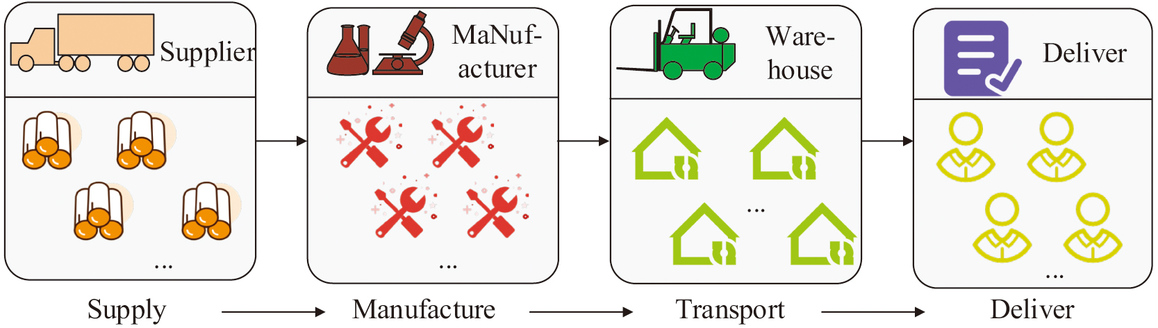Fig. 1. Schematic diagram of GSCN model application scenarios.

In Fig. 1, raw materials and manufacturing processes should possibly be considered in terms of their environmental impact and pollution emissions. The transportation process, as well as the product distribution and recycling process, should try to refine the carbon emissions of the product content that may generate pollution. The research design includes the GSCN objective function of raw material cost $Mat Cos t$ , manufacturing cost $\Pr o Cos t$ , fixed cost $Fixed Cos t$ , and freight cost $Fre Cos t$ , as shown in Equation (1).

\min O b j = Mat Cos t + \Pr o Cos t + F i x e d Cos t + F r e Cos t

(1)

In this case, the mathematical expression of the cost of raw materials is specified in Equation (2).

M a t Cos t = \sum_{p = 1}^{T Q} \sum_{s = 1}^{S p} \sum_{m = 1}^{M} S p r i_{p, s} \times Q S u p m_{p, s, m}

(2)

In the cost of raw materials in Equation (2), $p$ and $T Q$ denote the quantity of raw materials and type $S_{p}$ and the quantity of supplier $p$ . $M$ denotes the quantity of manufacturer $m$ . $S p r i_{p, s}$ is the unit price of raw materials supplied. $Q S u p m_{p, s, m}$ is the quantity of raw materials supplied to the manufacturer by the supplier. The manufacturing cost is calculated as shown in Equation (3).

\Pr o Cos t = \sum_{m = 1}^{M} N P M_{m} \times M p r i_{m}

(3)

In the manufacturing cost of Equation (3), $N P M_{m}$ is the number of products being manufactured, and $M p r i_{m}$ is the unit cost of manufacturing the product. The fixed cost is calculated as shown in Equation (4).

F i x e d Cos t = \sum_{m = 1}^{M} M S_{m} \times M f i x C_{m} + \sum_{w = 1}^{W} W S_{m} \times W f i x C_{w}

(4)

In the fixed cost of Equation (4), $W$ is the number of warehouses $w$ . $M S_{m}$ and $W S_{m}$ denote the manufacturer and warehouse being selected. $M f i x C_{m}$ and $W f i x C_{w}$ are the fixed costs of manufacturer and warehouse. The freight cost calculation is shown in Equation (5).

F r e Cos t = M a t Cos t + \sum_{m = 1}^{M} \sum_{w = 1}^{W} U t p C_{m, w} \times Q P p_{m, w} + \sum_{w = 1}^{W} \sum_{c = 1}^{C} U t p C_{w, c} \times Q P p_{w, c}

(5)

In the freight cost of Equation (5), $C$ denotes the number of customers $c$ . $U t p C_{m, w}$ and $U t p C_{m, w}$ are the transportation costs per unit of product from manufacturer $m$ to warehouse $w$ and warehouse $w$ to customer $c$ . $Q P p_{m, w}$ is the number of products supplied by the manufacturer to the warehouse. $Q P p_{w, c}$ is the number of products supplied by the warehouse to the customer. To ensure the realism of the GSCN model application scenarios, the research design assumptions and constraints: The ratio of supplied material materials should be in line with the actual production situation. Each part of the GSCN modeling process should have capacity constraints. That is, the number of products they supply shall not exceed the maximum demand. Customer demand is known in advance. Supply channels as well as production and delivery methods can be diverse [23,24]. It ensures that $Q S u p m_{p, s, m}$ , $Q P p_{m, w}$ , and $Q P p_{w, c}$ are integers. The condition for setting the supplier, manufacturer, and warehouse to be selected satisfies the binary constraint, that is, the range of its values should be {0,1}. The study also sets the green constraint. That is, the pollutant emission values of the supply $S p o l l u t i o n_{p, s}$ and manufacturing $M p o l l u t i o n_{m}$ are less than or equal to the criteria pollutant emission $P_{n o r m}$ , as shown in Equation (6).

\sum_{p = 1}^{T Q} \sum_{s = 1}^{S p} \sum_{m = 1}^{M} U t m C_{p, s, m} \times S p o l l u t i o n_{p, s} + \sum_{m = 1}^{M} N P M_{m} \times M p o l l u t i o n_{m} \leq \sum_{m = 1}^{M} N P M_{m} \times P_{n o r m}

(6)

B.PR-MPA-BASED DESIGN

The designed GSCN model contains more solution variables and constraints. To effectively deal with the solution conditions of this model, this study improves the solvability of the scheme with the help of MPA. Among them, MPA, as a population intelligence algorithm, solves the load optimization problem by simulating the foraging mechanisms, for example, Levi’s flight, Brownian motion, etc., of marine predators in search of prey [25]. The MPA completes the initialization through population individual initialization, individual fitness calculation, and position update. It is also iteratively optimized based on three predatory behaviors: high-speed chasing, cruising predation, and local roundup [26]. Moreover, the MPA also jumps out the local optimum with the help of fish aggregation device. When $r \leq F A D s$ , then the mathematical expression of predator ${\vec{\Pr e y}}_{i}$ is shown in Equation (7).

{\vec{\Pr e y}}_{i} + C F [{\vec{X}}_{\min} + \vec{R} ⊙ ({\vec{X}}_{\max} - {\vec{X}}_{\min})] ⊙ \vec{U}

(7)

When $r > F A D s$ , then it can be expressed as Equation (8).

{\vec{\Pr e y}}_{i} + [F A D s (1 - r) + r] \times ({\vec{\Pr e y}}_{r 1} - {\vec{\Pr e y}}_{r 2})

(8)

In Equations (7) and (8), $\vec{R}$ is a random vector. $r$ is the random number. $F A D s$ is the variable controlling the degree of influence of the fish aggregation device. $\vec{U}$ is the binary vector. $C F$ is an adaptive parameter controlling the predator step size. $i$ is the index. $⊙$ is the Hadamard product. ${\vec{X}}_{\max}$ and ${\vec{X}}_{\min}$ are the upper and lower bounds of the optimization problem. ${\vec{\Pr e y}}_{r 1}$ and ${\vec{\Pr e y}}_{r 2}$ are random integers of the predator [27]. The GSCN problem involves factors such as the number of raw materials being supplied, the number of products being supplied, the number being manufactured, and the probability of suppliers, manufacturers, and warehouses being selected. Therefore, in order to simplify the model, the study improves the MPA with stage fixes and improves the convergence of the algorithm in terms of path decision and freight allocation. The study designs a coding scheme consisting of three components: quantity of raw materials supplied, quantity of products supplied, and quantity manufactured. Moreover, this study analyzes them in terms of raw material availability, product transportation, and delivery. Considering that a large number of schemes can occur in the GSCN population, this study sets up stage detection to quickly locate the problem. The steps of stage detection are shown in Fig. 2.

Fig. 2. Stage detection step.

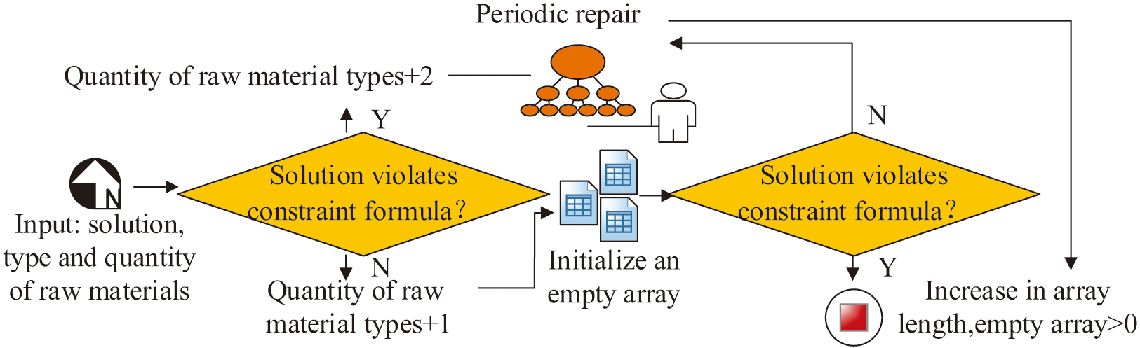
In Fig. 2, if the program violates the constraints, it is repaired in stages. The study controls the repair probability with the help of an adaptive parameter $λ_{r e p a i r}$ as shown in Equation (9).

λ_{r e p a i r} = 0.01 \times e^{(p l - 1)}

(9)

In Equation (6), $e$ is the Euler number, and $p l$ is the proportion of feasible solutions in the population. Different from the idea of stage repair that turns the constrained problem into an unconstrained problem with the help of an external penalty function, this study introduces a path decision operator and a freight allocation operator to realize the repair. That is, the path decision and freight volume of the solution are allocated until the constraints are satisfied. Among them, the path decision operator adopts binary encoding to represent the logistics path (0/1 indicates whether an edge is selected or not), and enhances the population diversity through random generation. The legitimacy verification rules for logistics paths are supply-demand matching and global equilibrium. That is, the total supply and the total supply of each demand side should be greater than the product demand and total demand. The path decision algorithm ensures solution feasibility by iteratively correcting illegal paths while maintaining search space diversity. The freight allocation operator, on the other hand, allocates logistics paths based on greedy ideas. Its primary consideration is to ensure that the supply can satisfy to meet the demand [28]. Figure 3 shows the schematic content of the phased repair operation.

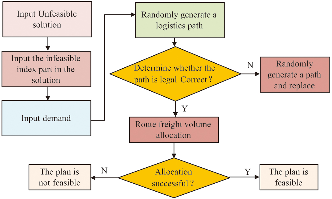Fig. 3. Schematic content of phased repair operation.

In the phased repair process in Fig. 3, a logistics path is randomly generated first. After that, it is judged whether it is legal or not according to the rules. If it is legal, then the freight volume can be allocated, otherwise, a randomly generated path is needed to replace the illegal part. When the freight allocation is successful, a feasible solution can be obtained. The PR-MPA can be obtained with the help of phased repair. The flow of the algorithm is shown in Fig. 4.

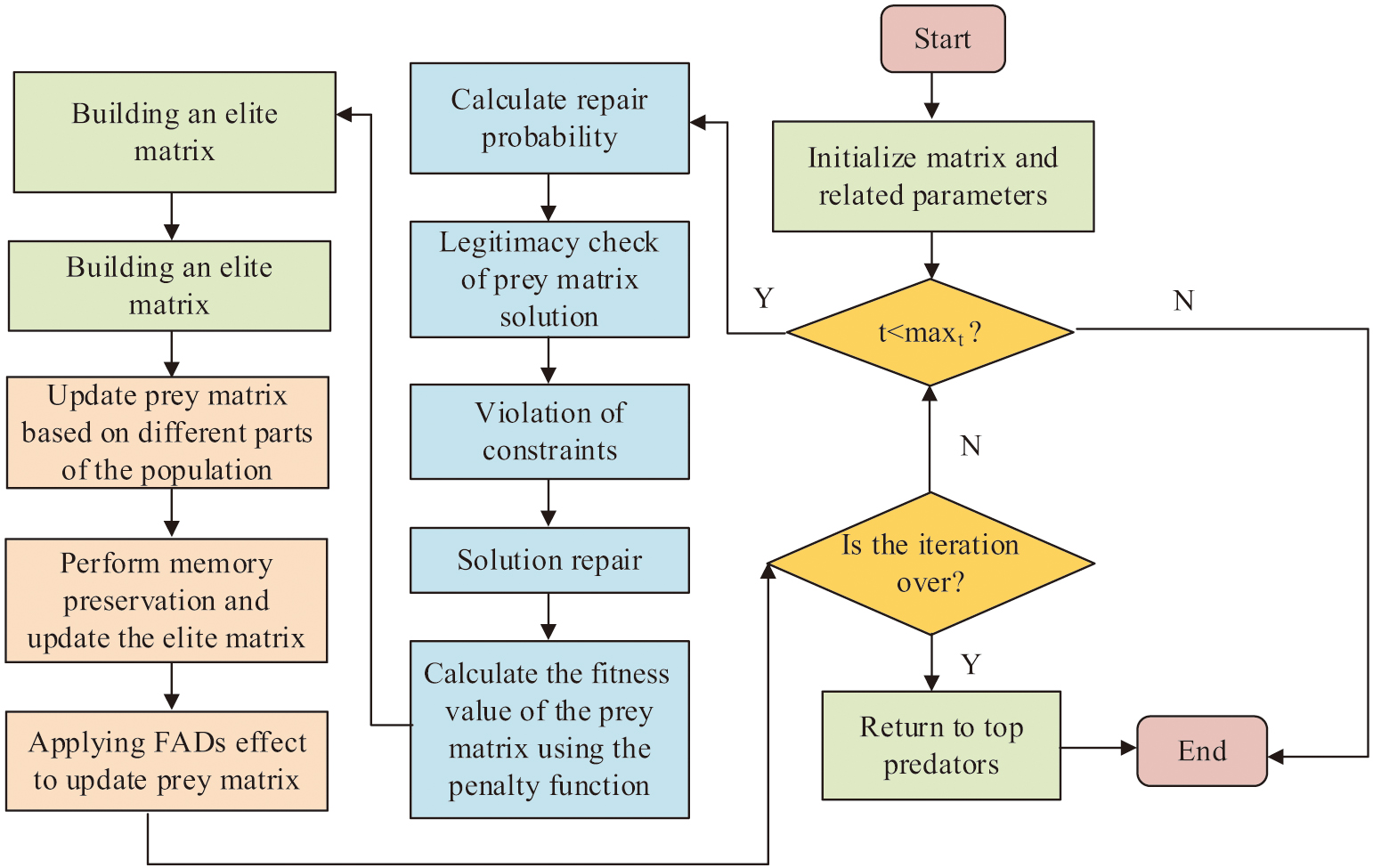Fig. 4. Schematic diagram of the process of improving the marine predator algorithm.

In Figure 4, the prey matrix is first initialized and relevant parameters are set. After that, the repair probability and legitimacy test are calculated in the iterative part. Path decisions and freights are assigned to the scenarios that violate the constraints to ensure that their scenarios are feasible. Afterward, the evaluation and MPA optimization phases are executed on the prey matrix to achieve the matrix update.

IV.ANALYSIS AND DISCUSSION OF GSCN INTELLIGENT OPTIMIZATION DESIGN RESULTS

The performance of the improved algorithm proposed by the study is tested with the help of commercial software tools (GAMS/XPRESS solver). The study is based on MATLAB 2019 to write a program to solve the GSCN objective function model. The experimental computer is configured with a Lenovo 2014 version (CPU: Intel Xeon Gold 6230 @ 2.1GHz, GPU: NVIDIA Tesla V100, 64GB DDR4 RAM). The programming language is Python 3.8. To test the application performance of PR-MPA, the study set up three different sizes of instance data for testing. Among them, in small-scale data, the number of manufacturers, warehouses, and customers is 4, 2, and 5, respectively. The number of test dimensions is 40, and the running time is 40s. In the medium-scale data, the number of manufacturers, warehouses, and customers is 5, 5, and 6, respectively. The number of test dimensions is 100, and the running time is 150s. In large-scale data, the number of manufacturers, warehouses, and customers is 8, 6, and 10, respectively. The number of test dimensions is 150, and the running time is 300s. The population size of the PR-MPA is set to 50, the maximum number of iterations is 200, the Levy flight parameter is 1.5, and the perturbation probability is 0.1. The PR-MPA is compared with non-dominated sorting genetic algorithm II (NSGA-II), multi-objective particle swarm optimization (MOPSO), multi-objective ant colony optimization (MOACO) for convergence and error results. The results are shown in Fig. 5.

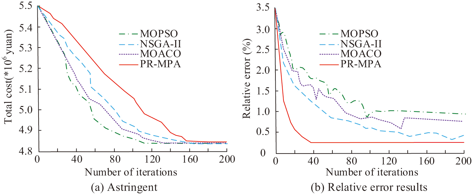Fig. 5. Convergence and error results of different algorithms for solving.

In Fig. 5(a), the total costs of the compared algorithms all show negative correlation with the number of iterations. Among them, the MOPSO algorithm has poor convergence curve performance. The fluctuation of the convergence curves of MOACO algorithm and the NSGA-III algorithm is obvious. Its cost convergence curve fluctuation is relatively small in the number of iterations more than 120 times. The PR-MPA has the fastest convergence rate. In Fig. 5(b), the PR-MPA exhibits an average error result of less than 0.25 and its curve changes are smoother in the later stage. Whereas the average errors of NSGA-II algorithm, MOACO algorithm, and MOPSO algorithm are all greater than 0.8, respectively. Their minimum errors reach 0.32, 0.58, and 0.88, respectively. The reason for the above results is that the improved idea of PR-MPA can help to jump out of the local optimum and accelerate the global convergence. Furthermore, its search mechanism is more suitable for the mixed problem of discrete and continuous variables in logistics networks [29]. NSGA-II algorithm can effectively maintain the solution set distributivity, so its convergence is higher than MOACO algorithm and MOPSO algorithm. However, its crossover and mutation tend to slow down the convergence speed [30]. MOPSO algorithm is more dependent on external archives and more sensitive to parameters. MOACO algorithm is difficult to weigh the conflicting goals in logistics path decision-making. This increases its computational complexity and affects the convergence speed and accuracy [31]. The average percentage deviation and average processing time of the above algorithms are analyzed under logistics data processing. The results are shown in Fig. 6.

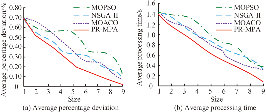Fig. 6. Average percentage deviation and average processing time of logistics data processing using different algorithms.

In Fig. 6(a), the PR-MPA exhibits the smallest average percentage deviation compared to the other algorithms. Its variation curve is smoother and its minimum value is less than 0.05%. Whereas, the NSGA-II algorithm, MOACO algorithm, and MOPSO algorithm have average percentage deviation greater than 0.06% and the curve fluctuation is obvious. In Fig. 6(b), the PR-MPA exhibits a shorter time cost in data processing. Its overall exhibited average processing time is less than 0.2s, which is much smaller than other comparative algorithms (greater than 0.3s). Afterward, the PR-MPA is compared on small and medium-scale instances (two test elements are selected for each instance). It is also compared with TS [9], Lagrangian relaxation fix-and-optimize (LR-FO) [10], Gaussian-improved marine predators algorithm (GIMPA) [15], and ANN [16]. The results are shown in Table I.

Table I. Comparison results of examples of different algorithms

Scale	Example	TS	LR-FO	GIMPA	ANN	PR-MPA
Small-scale	A	145930.1	147125.1	154407.2	146395.4	139537.5
		147355.7	147610.2	155507.9	3346512.3	139616.4
		149184.4	148490.7	156150.1	9145975.2	139673.2
	B	153024.3	154063.5	154687.1	154200.0	147568.1
		154026.5	154173.1	355121.3	1954316.3	148344.9
		154484.1	154258.3	1152447.1	6154623.1	148892.1
Medium-scale	A	215894.2	3.2E+12	226603.5	5.33E+12	204139.7
		221257.5	4.13E+12	233702	6.59E+12	205325.5
		226624.2	6.69E+12	238070.3	9.2E+12	206259.4
	B	218835.4	7.4E+12	227025	5.67E+12	205106.4
		224895.7	3.13E+13	235095.8	6.85E+12	206169.5
		230526.1	6.53E+13	238757.1	7.62E+12	208338.1

In Table I, under small-scale instances, the PR-MPA can find the optimal solution of the test instances better with the values of 139725.0 and 147056.3. The next better performers are the TS algorithm and the GIMPA. Whereas the ANN algorithm and GIMPA have poor searching ability, and their optimal values are much larger than 140,000. In medium size instances, PR-MPA has significantly better searching ability than other compared algorithms, and its optimal value is smaller than that of other algorithms, whereas ANN algorithm has significant constraints. After that, the convergence of the above algorithms is compared. The results are shown in Fig. 7.

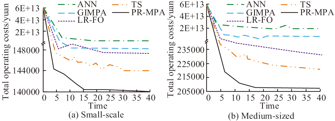Fig. 7. Convergence of different algorithms under different scale instances

In Fig. 7, the PR-MPA converges better than the other algorithms for both scale instances. Its total operating cost converges to 140,000 and 205,000 yuan. The next better performers are the TS algorithm and the LR-FO algorithm. The TS algorithm has convergence values greater than 144,000 and 220,000 yuan at small and medium sizes. The LR-FO algorithm has convergence values greater than 147,000 and 225,000 yuan for both algorithms. The faster convergence of ANN causes it to fall into convergence prematurely, making its convergence value much larger than that of the other comparative algorithms. The reason for the above result is that the forbidden table avoids repeated searches and is suitable for small-scale combinatorial optimization. However, the easy neighborhood search has difficulty covering the complex solution space and is more obviously affected by the initial solution. Therefore, its performance is slightly worse at medium scale [32]. Lagrangian relaxation is inefficient for simple constraints, and the accuracy of solving subproblems after decomposition is insufficient. Moreover, it is difficult to deal with multi-constraint coupling at medium-scale [33]. Although the Gaussian distribution adjusts the step size to improve the global search ability, it is insufficient in handling discrete variables [34]. The PR-MPA proposed in the study allows for stage detection and repair of the solution to ensure that it is better explored to a feasible solution. It reduces the running time and speeds up the convergence of the algorithm. After that, the solution set performance of the research algorithm is analyzed with the help of hypervolume (HV) metric. The larger the HV value, the better the convergence and diversity of the algorithm’s solution set. The results are shown in Table II.

Table II. Comparison results of HV for different algorithms

Scale	Example	TS	LR-FO	GIMPA	ANN	PR-MPA
Small-scale	A	763783	1069783	1199783	997783	1649783
		2049783	2379783	3959783	2499783	3889783
		2189783	2489783	3809783	2579783	4279783
	B	547783	487783	531783	341783	601783
		809783	740783	812783	565783	900783
		1379783	1189783	1449783	969783	1529783
Medium-scale	A	1519783	979783	658783	1569783	1289783
		1369783	816783	590783	1419783	1139783
		1299783	856783	544783	1339783	1109783
	B	1199783	725783	516783	1229783	999783
		1129783	706783	515783	1159783	924783
		1299783	816783	565783	1339783	1089783

In Table II, PR-MPA has the best results on the test instances. It is followed by TS algorithm and LR-FO algorithm, and the performance of the studied algorithms is relatively less affected by the dataset. The ANN algorithm, on the other hand, is more significantly affected, and its maximum values reach 2579783 and 1569783 at small and medium sizes. After that, the repair probabilities of different algorithms on the test instances are analyzed, and Table III is obtained.

Table III. Repair probability

Scale	TS	LR-FO	GIMPA	ANN	PR-MPA
Small-scale	18.25	24.55	23.36	15.23	35.33
Medium-scale	14.23	78.23	80.25	35.81	84.26
Large-scale	43.61	81.34	76.32	47.29	87.26

In Table III, the repair probability of different algorithms increases with the number of scales. Among them, the repair probabilities of TS, LR-FO, GIMPA, ANN, and PR-MPA on large-scale instances are 43.61%, 81.34%, 76.32%, 47.29%, and 87.26%, respectively. The research model has good repairability, which indicates that it can effectively improve the algorithm solution quality. Due to the potential for duplication in the optimal path search process of the improved MPA-SR algorithm, the study proposes analyzing its worst-case complexity. The results are shown in Table IV.

Table IV. Worst case complexity analysis results

Scale	Number of network nodes	Edges	Number of customer demands	Maximum number of iterations	Population size	Theoretical worst-case complexity (total (ms))	Actu-al average time (Avg (ms))
Small-scale	11	20	5	200	50	2.0 × 10⁵	198
Medium-scale	36	78	12	250	80	1.56 × 10⁶	1483
Large-scale	60	155	30	300	100	4.65 × 10⁶	3920

In Table IV, the theoretical worst-case complexity values for the three scales are 2.0 × 10⁵ ms, 1.56 × 10⁶ ms, and 4.65 × 10⁶ ms, respectively, which are much higher than the corresponding measured values of 198 ms, 1483 ms, and 3920 ms. It verifies the effectiveness of the early pruning and repair probability decay strategies in the algorithm. The effectiveness of the application of PR-MPA solving is analyzed with the help of time index (CPUT) and spacing index (SI). The results are shown in Fig. 8.

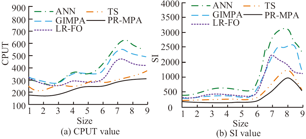Fig. 8. CPUT and SI values of different algorithms

In Fig. 8, the improved PR-MPA exhibits the shortest running time and smaller SI than the other algorithms. Its average CPUT and SI values reach 276 and 717, which are much smaller than those of the other algorithms compared. The maximum values of CPUT and SI of the ANN algorithm are more than 600 and 3000. In conclusion, the research method can be better applied to sustainable network optimization design. After that, the solution set results of the above algorithms are analyzed. The results are shown in Fig. 9.

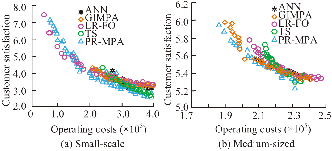Fig. 9. Solution set results of different algorithms.

In Fig. 9, the PR-MPA’s solution set results are closer to the axes, indicating that it is better able to balance the cost and customer satisfaction issues. The next better performers are the LR-PO algorithm and the TS algorithm. The GIMPA and the ANN algorithm have fewer solution sets under the objective space, indicating that their processing is less effective.

V.CONCLUSION

The study designed the GSCN taking into account the pollution emission and capacity constraints. The results indicated that the PR-MPA exhibited less convergence and error values, and its average error turned out to be less than 0.25. In contrast, the NSGA-II, MOACO, and MOPSO algorithms all had an average error of more than 0.8, respectively, and there was a significant node fluctuation in the convergence curves of the comparative algorithms. In the logistics data processing results, the PR-MPA showed a minimum average percentage deviation of less than 0.05% compared to the other algorithms, and the average processing time was less than 0.2 s. The average percentage deviation of the PR-MPA was less than 0.05% compared to the other algorithms. In contrast, the NSGA-II algorithm, MOACO algorithm, and MOPSO algorithm, all had average percentage deviations greater than 0.06% and average processing times greater than 0.3s. The PR-MPA converged better than the other algorithms for both scale instances in the example results. Its total operating cost of small and medium-sized enterprises converged to 140,000 yuan and 205,000 yuan, respectively. The next better performers were the TS algorithm and the LR-FO algorithm. The TS algorithm converged to values greater than 144,000 and 220,000 yuan at small and medium sizes. The convergence values of LR-FO algorithm in small and medium scales were both greater than 147,000 yuan and 225,000 yuan, respectively. The PR-MPA exhibited the shortest running time and smaller SI than the other algorithms. Its average values of CPUT and SI reached 276 and 717, respectively, which were much smaller than the other algorithms compared. The maximum values of CPUT and SI for ANN algorithm were more than 600 and 3000. Moreover, the solution set results of PR-MPA were closer to the axes, which indicated that it was able to balance the cost and customer satisfaction issues better. The next better performers were the LR-PO algorithm and the TS algorithm. The GSCN designed by the research method could balance economy and environmental protection for decision optimization and solution management.

However, the research method spends a long time in dealing with large-scale problems and does not consider issues such as transportation carbon emissions. At the same time, research faces challenges such as frequent calls to repair operators in large-scale instances. This leads to an increase in iteration time and an exponential growth of binary extension variables in multi-period random environments. The research method is combined with other deep learning algorithms, IoT technologies, etc. Moreover, the introduction of life cycle and other theories to quantify the environmental impact of logistics supply chain networks is an important research direction in the future.

Intelligent Optimization Design of Green Logistics Supply Chain Network Considering Pollution Emission and Capacity Constraints