I.INTRODUCTION
The Internet of Things (IoT) refers to any object with sensors and stimuli that contain and transmit information to other systems, programs, or applications [1]. The advantages of IoT devices have boosted the use of gadgets at an exponential level due to a wide application across different industries [2]. For example, in smart transportation, technologies enabled by IoT, such as advanced driver assistance systems, contribute toward minimizing incidents because of humans [3]. The intrusion detection system (IDS) plays a critical role in ensuring network security by handling large data streams and providing prompt responses, making it highly effective for real-time applications [4]. By incorporating artificial intelligence (AI), IDS identifies intrusion in a network by analyzing both deterministic and probabilistic behavior [5]. In most cases, network flow contains legitimate data movements, but sometimes arbitrary activity that provokes service disruptions is also seen [6]. Moreover, the malicious behavior category usually contains data that is influenced by known attack patterns. IDS are broadly classified into two types: Network IDS (NIDS) and Host IDS (HIDS) [7]. NIDS maintains continuous surveillance of network traffic, which itself is a target of several attacks, and HIDS works on network devices for host-level analysis of malicious activities [8].
The IDS is crucial to the defense of network traffic legitimacy, as it can identify internal and external invasions in real time [9]. Structurally, they are combined with firewalls to mitigate complex network threats and are interfaced with alarms to deter unlawful actions [10]. In the operation, the specification-based IDSs identify threats through traffic analysis that matches them with the standard set of rules and specifications created by professionals [11]. In this case, the anomaly-based IDSs are continuously monitoring the network activities to identify some unusual patterns in the network’s activities [12]. In the past few years, improvements have been made in ML, especially the supervised deep learning techniques that have improved NIDS [13]. ML-based IDSs fall into two categories such as supervised and unsupervised learning [14]. The ML techniques being used here include both the supervised and unsupervised techniques such as Random Forest (RF), Decision Tree (DT), Hidden Markov Model (HMM), and K-means [15]. However, a few issues are still unsolved, such as the real-time detection, treatment of class imbalance problem, concerns of quality, high dimensionality and feature space, huge incoming data, and time performance [16]. Despite significant progress in IDS for IoT networks, the existing research faces challenges such as redundant attributes, higher-dimensional feature spaces, and computational overhead that affect the model performance. Furthermore, the traditional ML struggled to capture complex temporal and spatial dependencies of dynamic IoT, thereby leading to reduced accuracy and high false alarms. These limitations motivate the need for a lightweight and accurate IDS that operates effectively in resource-constrained IoT environments. To address these limitations, the Lyrebird Optimization Algorithm (LOA)-Beta Hebbian Learning-based Elite Spike Neural Network (BHLESNN) was developed to integrate LOA for optimal feature selection, thereby minimizing redundancy and dimensionality with BHLESNN to improve temporal encoding and stabilize the classification. This combination is significant as it not only attains higher detection accuracy among benchmark datasets but also ensures robustness and fewer false positives for real-time IoT deployments where precision and efficiency are significant. The main contributions are stated as follows:
- •The hash encoding converts the categorical features into integer format with the help of a hash function. The min-max normalization process is utilized to standardize each variable into the same range of values to eliminate the indicators of large scales from taking over the features of other variables.
- •The LOA selects optimal features and reduces redundancy because it can explore and exploit the search space, thereby enhancing classifier performance.
- •The BHLESNN utilizes the Hebbian learning rule to adaptively strengthen the connections based on input data correlation patterns, thereby enhancing the network’s ability to identify complex attacks.
- •The usage of the beta function for spike encoding enhances the temporal precision and allows a better presentation of dynamic features in network traffic.
This research paper is given as follows: Section II investigates the literature review, and Section III elaborates the proposed method. Section IV specifies the result analysis, and the conclusion of this research paper is given in Section V.
II.LITERATURE REVIEW
This section discusses the recent research based on IDS classification in IoT using deep learning (DL) techniques, with its process, advantages, and limitations.
Silivery et al. [17] designed a DPFEN used for categorized network attacks on IoT devices. The DPEFN was used to enhance feature extraction and fusion procedure through integrating a Convolutional Neural Network (CNN) and an Improved Transform Network (ITN). The Neural Architecture Search Network (NASNet)-based classifier was used to perform IDS. The DPFEN method might not account for the possibility of attacks that target an IDS.
Elsayed et al. [18] developed a Secured Automatic Two-level Intrusion Detection System (SATIDS) using enhanced Long Short-Term Memory (LSTM) to differentiate between attacks and benign traffic while identifying the specific attack category. The Rectified Linear Unit (ReLU) activation system performed a threshold operation for an input element about zero, as input data comprises negative values. The ReLU layer passes a positive input and provides a zero value for a negative input. The IoT devices have limited energy and computational resources, which makes it a challenge without significant resource optimization.
Mahalingam et al. [19] presented a Range-Optimized Attention Convolutional Scattered Technique (ROAST-IoT) to prevent threats and intrusions. The model used a scattered range feature selection (SRFS) to identify a significant property from supplied data. The attention-based convolutional feed forward network (ACFN) was used to identify an IDS. The Modified Dingo Optimization (MDO) was applied for enhanced accuracy of the classifier. The DMO algorithm ensures optimal classifier performance under dynamic network and attack conditions.
Gaber et al. [20] introduced an Innovative IDS based on DL for detecting attacks. The Kernel Principal Component Analysis (KPCA) was applied to detect the attack feature extraction, and CNN was used for recognition and classification. The usage of KPCA was unable to minimize the processing time and help enhance the attack detection rate. The combination of KPCA and CNN increased the processing latency, which affects a system’s ability to perform real-time attack detection.
Anushiya and Lavanya [21] introduced a Genetic Algorithm Faster Recurrent Convolutional Neural Network (GA-FR-CNN) used for IDS. The GA-FR-CNN was used to recognize an IDS in DL. An Assimilated Artificial Fish Swarm Optimization (AAFSO) reduced the memory and cost of feature selection through GA-GR-CNN for effective classification to attain an attack detection. The performance of AAFSO and GA relies on hyperparameter tuning, which consumes time and presents challenges to optimize for various network conditions.
From the above analysis, the high processing latency affects a system’s ability to perform real-time attack detection, consumes time, and challenges optimization for various network conditions, might not account for the possibility of attacks that target an IDS, and is limited by energy and computational resources, which pose challenges without significant resource optimization.
III.PROPOSED METHOD
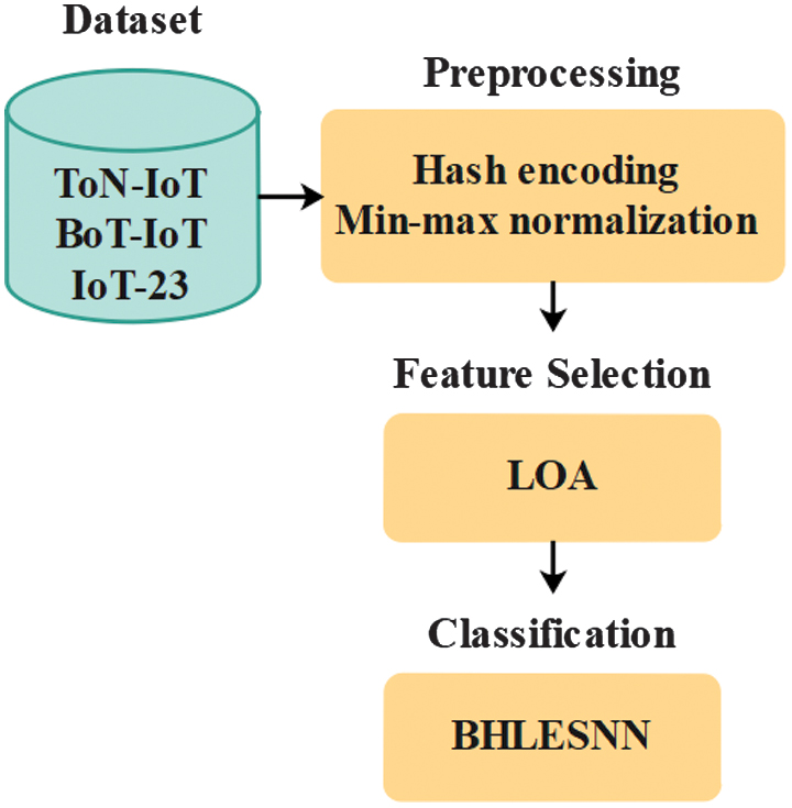
In this research, LOA-BHLESNN is proposed for a classification of IDS, which classifies the network traffic into multiple classes. Primarily, the three datasets, including ToN-IoT, BoT-IoT, and IoT-23, are considered to estimate the LOA-BHLESNN effectiveness. The hash encoding and min-max normalization are applied as preprocessing, which converts the categorical features into integer format, and then the features are normalized. The LOA is applied to select the best set of features through the exploration and exploitation stage. Finally, the selected features are given to BHLESNN to improve the classification accuracy. Fig. 1 shows the workflow of IDS.
A.DATASET
The ToN-IoT [22], BoT-IoT [23], and ToT-23 [24] datasets are applied in this research, which are publicly available Kaggle datasets. A detailed explanation of these datasets is given below:
ToN-IoT: This dataset integrates internet streams of 22,339,021 collected through the IoT ecosystem, with a ratio of 21,542,641 intrusions and 796,380 regular network flows. This dataset is used to retrieve 44 different features, and it includes various attacks, including ransomware, DoS, injection, Man in the Middle (MITM), Cross-Site Scripting (XSS), Benign, Password, Backdoor, DDoS, and scanning.
BoT-IoT: This dataset is formed to accomplish feature selection and precisely identify Bot attacks in IoT networks. It has 46 features and various attacks, including normal, theft, DDoS, DoS, and reconnaissance.
IoT-23: This dataset comprises 3 benign traffic captures and 20 malicious traffic grabs in which malicious traffic was generated by replicating various attacks. The dataset contains log files generated through the Zeek network analyzer and composed network files. This dataset contains 21 features with label data and 325,307,990 records.
B.PREPROCESSING
The three datasets are preprocessed using two techniques: hash encoding and normalization [25]. When working with categorical features, hash encoding is used to transform values into an integer format with the help of a hash function. This technique maps categorical feature space to a high dimension of numerical space while preserving distances between the vectors of categorical features. Min-max normalization process is utilized to standardize every variable by scaling in the same range to eliminate the indicators of large scales from dominating the features of other variables. It scales the values for each feature between 0 and 1 based on Eq. (1):
where is a normalized feature, is an actual feature, and and are the minimum and maximum number of features.C.FEATURE SELECTION
The Lyrebird Optimization Algorithm (LOA) [26] is a population-based heuristic algorithm where lyrebirds establish an appropriate solution for optimization by searching the influence of its members. Every lyrebird in LOA acts as a member that controls decision variable values according to its location. Hence, each lyrebird is modeled by a vector in which every element of its vector presents a decision variable from a mathematical view. The primary location of LOA members in the problem-solving space is adjusted by Eq. (2):
where is a random number in , and and are lower and upper bound of decision variable , respectively. The objective functions are better criteria for calculating the candidate solution quality. The best estimated score for the objective function is based on the optimal candidate solution, while the worst estimated score relates to the worst candidate solution. In every iteration, the lyrebird positions are updated, and the optimal candidate solution is refined according to the objective function. Based on Lyrebird’s decision in this condition, the population update procedure has a dual strategy such as escaping and hiding. In LOA, the lyrebird’s decision-making process involves selecting either an escape or hiding strategy based on the danger, which is replicated in Eq. (3): where is a random number from [0, 1].1).EXPLORATION PHASE (ESCAPING STRATEGY)
In this LOA, the population member’s location is updated in the search space according to the lyrebird’s escape from a dangerous position to a safer area. Once moved to a safer region, it leads to high changes in location and scanning of various regions, which denotes the exploration capability of LOA in global search. In LOA, every member location of other population members has optimal objective functions, which are taken in safer areas. Hence, safer area set for every LOA member is determined by Eq. (4):
where is a group of safer areas for lyrebird and is a th row of matrix that has the best objective function value compared to LOA members. In LOA, it is considered that the lyrebird escapes to safer regions. According to the lyrebird movement, a new location is estimated for every LOA member by Eq. (5). If the objective function is an improvement, the new location changes the earlier location of the respective member based on Eq. (6): where is a designated safe region for lyrebird , is a new location estimated for th lyrebird according to its escaping strategy, is its dimension , is its objective function score, is a random number from [0, 1], and is a numbers which are selected randomly as 1 or 2.2).EXPLOITATION PHASE (HIDING STRATEGY)
In this step, every population member updates its location within the search space, which mimics the lyrebird’s method of hiding in its nearest safer region. The lyrebird scans its environment as carefully as possible, making small movements to find a suitable position to hide, which only slightly shifts its placement, paralleling LOA’s exploitative nature. By considering the movement of the lyrebird toward a better hiding area, each LOA member updates the new position by Eq. (7). The update rule of lyrebird escape and hiding behavior ensures balance among global exploration and local exploitation. This dual-phase search avoids local optima and identifies high discriminative features in high-dimensional data. If updated, one improves the objective function value as in Eq. (8); this position succeeds the previous one:
where is a new location estimated for th lyrebird according to the hiding strategy of LOA, is its th dimension, is its objective function, is a random number from [0, 1], and is an iteration count. The LOA selects optimal features and reduces redundancy because it can explore and exploit the search space, thereby enhancing classifier performance. Its adaptiveness ensures that the balance among exploration and exploitation allows to avoid local optima and recognize discriminative features. The selected features provide better and more accurate detection of various intrusion patterns, thereby enhancing the overall model performance. The LOA is suitable for feature selection in IDS due to its ability to address the challenges from high-dimensional and highly correlated IoT network data. Its dual phase enables LOA to scan feature space for globally relevant features while refining the subset to enhance the detection performance. These balances help avoid local optima that arise from redundant features, thereby ensuring the selection of features that are truly discriminative for separating benign and malicious traffic. Moreover, the adaptive position of the LOA update mechanism makes it better to adjust the feature subset to evolving attack signatures that are significant for dynamic network environments. Through generating a minimal, highly informative feature set, the LOA reduces the classifier, thereby enabling BHLESNN to learn temporal-spatial patterns effectively. In this research, the LOA is configured with the following main parameters to optimize the network weights. The population size was set to 30, which denotes the number of candidate solutions explored in every iteration. The algorithm was executed for a maximum of 100 iterations, which is considered the stopping criterion unless convergence was reached earlier. Fig. 2 shows the flowchart of LOA.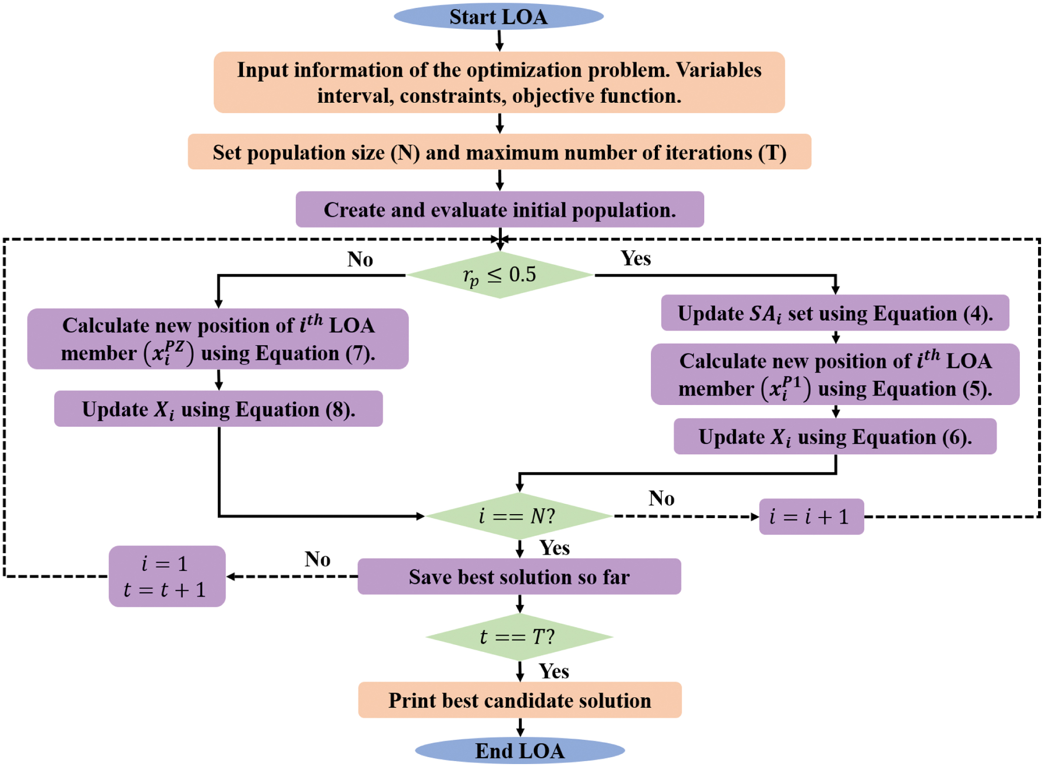
D.CLASSIFICATION
This kind of partially recurrent Spiking Neural Network (SNN) incorporates the simple Elman Neural Network (ENN) topology, which contains input, hidden, context, and output layers as defined in the ENN model. Self-feedback with a tunable gain factor is used in a context layer to save the previous output of the hidden layer while concurrently providing positive feedback. Because of this architecture, which is relatively light, the ESNN is especially amenable to compute intensive operations in embedded systems. The nodes of the input layer are designated by Eq. (9):
Consider , where is a th iteration, is input, and is a result of the initial layer. The ESNN dynamic is labeled in Eqs. (10)–(12):
where is an arbitrary nonlinear function that determines the organization and presentation of the EESNN. So, the input and the output are indicated through , which stands for output. For hidden and context layers, state node vectors are represented with and , respectively. The symbols of and express the weights between neurons of the first intermediate layer linked to the data layer. Here, the parameter of self-connective feedback gain is marked as , while weights interconnect output neurons with hidden layer outputs are marked as . The hidden layer is presented in Eqs. (13) and (14): where is a sigmoid function, are data from input and hidden layers, and is an output of hidden layer. Then, nodes within a context level are presented with respect to the layer as shown in Eq. (15):Here, signifies the self-connecting feedback gain, which is propagated in the context layer for adequate materialization of the required classification of the IDS. The self-feedback gain conserves temporal patterns from previous hidden outputs, thereby enabling ESNN to retain short-term memory required for sequential IDS traffic with less computational overhead. Each connection between layers in the ESNN is developed to include some terminals, where each of the terminals has its own set of weights and delays for each sub-connection. In the hidden layer of the ESNN architecture, there are only two input neurons and two output neurons. The outputs of nodes are determined at the end of the output layer as shown in Eq. (16):
where is a parameter which is managed through ESNN as shown in Eq. (17):The behavior of nodes in hidden layer is described through a formula and representing neural weights threading through the hidden layer outputs and neurons in other layers. The network connection statistics dynamically adapt to meet the requirements for best performance. The final stage of categorization is defined using Eq. (18):
In this model, is used to symbolize learning rate, while symbolizes unit of time frame. The value neuron threshold determines IDS classification according to the spiking during the period . This means that the threshold values fixed on the neurons are capable of distinguishing between normal activity and attacks. Membrane potential is considered into specific attack groups when it goes beyond a certain limit, and then specific groups of attacks are identified. This shows the delta function of neurons by , and it is possible for accurate categorization of IDS by using Eq. (19). The difference between final neurons is estimated by Eq. (20):
This equation estimates the deviations in actual vs predicted spike time, thereby guiding synaptic adjustments to enhance temporal-spatial patterns without retaining, where is a duration of neuron spike and is a result of the neuron’s actual spike time. The BHL utilizes a beta distribution as a portion of its weight update procedure to plan higher-dimensional datasets into low-dimensional subspaces for data extraction. In contrast to other examining approaches, the BHL provides a better presentation of internal structure. The BHL learning rule includes beta distributions to update weights by associating probability density function (PDF) of residual by dataset distribution. The residual denotes a difference between the input and output feedback by weights, and the optimal cost function is defined through the residual PDF. Hence, the residual is expressed by beta distribution parameters as shown in Eq. (21):
Where, alpha (α) and beta (β) control the shape of the probability density function (PDF). e is residual, x is a network input, W is the weight matrix, and is a network output. The beta distribution is adopted due to its bounded [0, 1] which matches the normalized residuals from spike responses. Its shape parameters and are flexible to adapt to the statistical nature of IDS. This enables accurate temporal encoding, thereby updating informative regions and suppressing noise, thereby outperforming fixed update of ESNN rules. Lastly, gradient descent is applied to enhance the weight as in Eq. (22):Therefore, the BHL denotes through the Eq. (23)–(25):
where is the learning rate. These equations integrate the beta PDF into Hebbian weight updates, thereby providing data-driven convergence. By modeling residual error distributions, the network update is selectively applied, thereby enhancing detection accuracy. The adaptive nature of ESNN ensures robustness against attack patterns in IDS. The ESNN supports incremental learning that is valuable for updating IDS continuously without retaining it entirely. The BHLESNN leverages the Hebbian learning rule to strengthen the connection adaptively based on correlation patterns of input data, thereby enhancing the network’s ability to identify complex attacks. Furthermore, its elite mechanism ensures optimal neuron selection, which enhances the classification performance and reduces false positives. This adaptability and robustness ensure the effectiveness of IDS in a highly dynamic network environment. Figure 3 shows the architecture of BHLESNN, showing forward inference and post-output learning with elite neuron selection.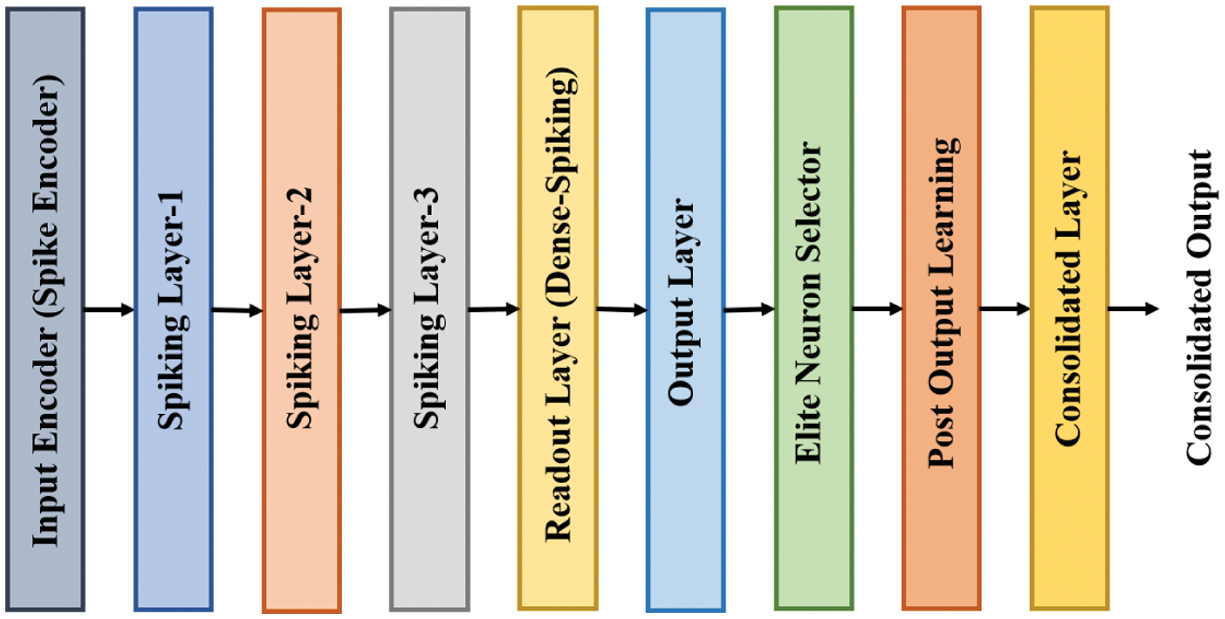 Fig. 3. Architecture of BHLESNN, including spike encoding, hierarchical spiking layers, elite neuron selection, and post-learning consolidation.
In BHLESNN, the ESNN is retained for its temporal memory capability, but the conventional Hebbian weight update is replaced with the BHL rule. This happens during the synaptic weight update after the neuron fires, where the BHL adjusts the weights using the beta PDF of residual error among predicted and actual spike responses, thereby providing adaptive and accurate temporal-spatial learning. Furthermore, the elite mechanism selects the fixed propagation of higher performing neurons at every epoch, thereby preserving the learned weights. This approach stabilizes training, prevents loss, and guides learning toward underperforming neurons, thereby enhancing the detection accuracy in IDS. The hyperparameters in Table I are selected by tuning and preliminary experiments on validating subsets of ToN-IoT, BoT-IoT, and IoT-23 datasets to balance detection accuracy, convergence speed, and computational efficiency. The 80:20 validation split was applied, and grid search with predefined ranges is combined with manual fine-tuning. The parameters such as learning rate, decay factor, and regularization are adjusted based on validation performance to prevent overfitting and ensure stable convergence. The activation function includes Sigmoid in hidden layers and a beta function for spike encoding, with the top 10% of neurons retained as elite neurons to improve learning ability. The maximum of 100 epochs is selected to enable learning without overfitting, to enhance performance. The batch size of 32 provides a trade-off between gradient estimation and memory usage. The Adam optimizer is selected for its adaptive learning rate ability, which enhances the convergence in higher-dimensional feature spaces. The initial learning rate is set as 0.01 with a learning rate drop factor of 0.99 and a gradient decay factor of 0.9 applied to reduce the step size for fine-grained weight adjustments. The gradient decay factor managed the moving average of past gradients, thereby enhancing the weight update stability, while the L2 regualirzation ranges within 0.001 helps to prevent overfitting by penalizing large weights. Overall, these parameters ensure that the BHLESNN maintains higher classification accuracy while minimizing false positives and training time.
Table I. Parameters and its values
| Parameters | Values |
|---|---|
| Maximum epoch | 100 |
| Batch size | 32 |
| Optimizer | Adam |
| Initial learning rate | 0.01 |
| Learning rate drop factor | 0.99 |
| Gradient decay factor | 0.9 |
| L2 regularization | 0.001 |
| Activation function | Sigmoid (hidden), beta function (spike encoding) |
| Validity split | 80:20 |
| Early stopping | 10 epochs |
| Elite neuron percentage | Top 10% retained |
The pseudocode of the proposed method is given below for reproducibility.
Input: Dataset
Output: Trained LOA-BHLESNN model
1. Preprocessing
Apply hash encoding to categorical features in .
Apply min-max normalization to scale all features to [0, 1].
2. Feature Selection using LOA
Initialize population of lyrebirds with random feature subsets.
Evaluate fitness of each subset using a validation classifier.
For each iteration:
For each lyrebird:
Generate random number r ∈ [0, 1].
If
Else Hiding Strategy
Update position using respective equations.
Evaluate new fitness; replace if improved.
Return optimal feature subset .
3. Classification using Beta Hebbian Learning Elite SNN (BHLESNN):
Initialize ESNN architecture (input, hidden, context, output layers).
Encode inputs using beta function for spike timing.
Set firing threshold θ = 0.5 and elite neuron selection parameter k = 10% of total neurons
Perform hyperparameter tuning:
Define candidate values for learning rate, decay factor, regularization coefficient, and elite ratio
Use k-fold cross-validation on training data to select the best combination
For each training epoch:
Forward pass: compute hidden/context states and outputs.
Compute residuals between predicted and actual spikes.
Update synaptic weights using the Beta Hebbian Learning rule:
Apply Elite mechanism:
Rank neurons by accuracy contribution
Retain top-k neurons and freeze their weights
Update remaining neurons
If membrane potential :
Classify as attack
Else:
Classify as benign
4. Evaluation:
Evaluate trained BHLESNN model on test data using selected features
Report accuracy, precision, recall, F1-score, training time, inference time, and memory usage
Return trained BHLESNN model.
IV.RESULT ANALYSIS
The LOA-BHLESNN effectiveness is analyzed in this research with the Python tool and the configurations of RAM 16GB, Windows 11 OS, Intel i9 processor, and GPU of NVIDIA GeForce RTX 3060/RTX 3070. The metrics, including precision, accuracy, F1-score, and recall, are assessed to show the efficiency of LOA-BHLESNN. The mathematical formula for these matrices is specified in Eq. (26)–(29):
where , and are True Positive, True Negative, False Positive, and False Negative, respectively.In Table II, the result analysis of optimization is provided with the metrics of precision, accuracy, F1-score, and recall for ToN-IoT, BoT-IoT, and IoT-23 datasets. The Coot Optimization Algorithm (COA), Kookaburra Optimization Algorithm (KOA), and Parrot Optimization Algorithm (POA) are analyzed and compared with the proposed LOA. The LOA achieves accuracy of 99.96%, 99.94%, and 99.81% for ToN-IoT, BoT-IoT, and IoT-23 datasets, respectively.
Table II. Result analysis of optimization
| Dataset | Method | Precision (%) | Accuracy (%) | F1-score (%) | Recall (%) |
|---|---|---|---|---|---|
| ToN-IoT | COA | 99.78 | 99.87 | 99.80 | 99.84 |
| KOA | 99.81 | 99.90 | 99.83 | 99.86 | |
| POA | 99.84 | 99.93 | 99.86 | 99.89 | |
| LOA | 99.87 | 99.96 | 99.89 | 99.92 | |
| BoT-IoT | COA | 99.64 | 99.85 | 99.74 | 99.85 |
| KOA | 99.67 | 99.88 | 99.77 | 99.88 | |
| POA | 99.70 | 99.91 | 99.80 | 99.91 | |
| LOA | 99.72 | 99.94 | 99.82 | 99.93 | |
| IoT-23 | COA | 99.68 | 99.72 | 99.63 | 99.60 |
| KOA | 99.71 | 99.75 | 99.66 | 99.63 | |
| POA | 99.73 | 99.78 | 99.68 | 99.65 | |
| LOA | 99.75 | 99.81 | 99.71 | 99.68 |
In Table III, the result analysis of the classifier with actual features is provided with the metrics of precision, accuracy, F1-score, and recall for ToN-IoT, BoT-IoT, and IoT-23 datasets, respectively. The RNN, SNN, and ESNN are analyzed and compared with the proposed BHLESNN. The BHLESNN achieves the accuracy of 99.93%, 99.92%, and 99.78% for ToN-IoT, BoT-IoT, and IoT-23 datasets, respectively.
Table III. Result analysis of classifier with actual features
| Dataset | Method | Precision (%) | Accuracy (%) | F1-score (%) | Recall (%) |
|---|---|---|---|---|---|
| ToN-IoT | RNN | 99.76 | 99.85 | 99.78 | 99.82 |
| SNN | 99.79 | 99.88 | 99.81 | 99.85 | |
| ESNN | 99.82 | 99.91 | 99.84 | 99.88 | |
| BHLESNN | 99.85 | 99.93 | 99.87 | 99.90 | |
| BoT-IoT | RNN | 99.62 | 99.83 | 99.72 | 99.84 |
| SNN | 99.65 | 99.85 | 99.75 | 99.87 | |
| ESNN | 99.68 | 99.88 | 99.78 | 99.89 | |
| BHLESNN | 99.70 | 99.92 | 99.80 | 99.91 | |
| IoT-23 | RNN | 99.65 | 99.71 | 99.61 | 99.59 |
| SNN | 99.68 | 99.73 | 99.64 | 99.61 | |
| ESNN | 99.71 | 99.75 | 99.66 | 99.63 | |
| BHLESNN | 99.73 | 99.78 | 99.68 | 99.65 |
In Fig. 4, the result analysis of the classifier with optimized feature is provided with the metrics of precision, accuracy, F1-score, and recall for ToN-IoT, BoT-IoT, and IoT-23 datasets, respectively. The RNN, SNN, and ESNN are analyzed and compared with the proposed BHLESNN. The BHLESNN achieves accuracy of 99.96%, 99.94%, and 99.81% for ToN-IoT, BoT-IoT, and IoT-23 datasets, respectively.
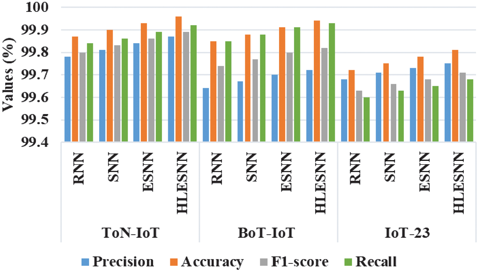 Fig. 4. Result analysis of classifier with optimized features.
Table IV presents the computational and statistical analysis of RNN, SNN, ESNN, and BHLESNN classifiers on ToN-IoT, BoT-IoT, and IoT-23 datasets. All p-values from the ANOVA test are less than 0.05, thereby ensuring the model is statistically significant in performance. The p-value from ANOVA was used as it was specifically developed to compare the multiple groups simultaneously, enabling the determination of whether there are statistically significant differences in model performance among various experimental settings. The other tests, such as the t-test, are limited to pairwise comparisons, whereas the ANOVA effectively handles multiple classes in a single analysis and provides an overall significant measure. The ESNN-based models, specifically BHLESNN, provide less training and inference time as well as reduced memory usage compared to other baseline models. Additionally, BHLESNN has a lightweight architecture with only 0.063 M trainable parameters that contribute to its computational efficiency. It required only 575 MB of memory on this configuration, thereby demonstrating its efficiency. The BHLESNN achieves less training time of 155.3 s, 170.5 s, and 140.7 s on ToN-IoT, BoT-IoT, and IoT-23 datasets, respectively. This ensures that the BHLESNN achieves computationally lightweight and suitable for resource-constrained environments than conventional baseline models by addressing higher inference time and memory usage. Given its lower parameter count and memory usage, the BHLESNN is feasible to deploy on lower-end edge devices, thereby making it better for IoT environments.
Table IV. Complexity and statistical analysis of classifier on different datasets such as ToN-IoT, BoT-IoT, and IoT-23
| Dataset | Method | Training time (s) | Inference time (s) | Memory usage (MB) | Parameter count (M) | P-value from ANOVA |
|---|---|---|---|---|---|---|
| ToN-IoT | RNN | 200.5 | 160.2 | 650 | 0.098 | 0.006 |
| SNN | 210.8 | 155.6 | 670 | 0.085 | 0.006 | |
| ESNN | 190.2 | 150.3 | 640 | 0.076 | 0.005 | |
| BHLESNN | 155.3 | 120.6 | 575 | 0.063 | 0.003 | |
| BoT-IoT | RNN | 185.7 | 145.4 | 620 | 0.098 | 0.004 |
| SNN | 195.3 | 140.8 | 630 | 0.085 | 0.004 | |
| ESNN | 175.9 | 135.6 | 610 | 0.076 | 0.003 | |
| BHLESNN | 170.5 | 110.3 | 590 | 0.063 | 0.004 | |
| IoT-23 | RNN | 180.6 | 130.2 | 605 | 0.098 | 0.003 |
| SNN | 185.9 | 125.5 | 615 | 0.085 | 0.003 | |
| ESNN | 165.4 | 115.8 | 595 | 0.076 | 0.004 | |
| BHLESNN | 140.7 | 95.1 | 550 | 0.063 | 0.002 |
Table V presents the cross-dataset evaluation results where the models are trained on BoT-IoT dataset and tested on IoT-23 datasets. BoT-IoT with a larger number of features is selected for training as it provides a higher and more varied representation of network behaviors, thereby enabling the model to learn a wider range of discriminative patterns. The IoT-23 dataset is considered for training because it has a smaller number of features compared to ToN-IoT, which represents the unseen environments. The proposed BHLESNN achieves better performance with 75.63% precision, 90.42% accuracy, 77.66% F1-score, and 79.82% recall, thereby outperforming the RNN, SNN, and ESNN. These results ensure that BHLESNN shows better discriminative feature selection and an adaptive Beta Hebbian weight update, thereby ensuring robust detection.
Table V. Analysis of different classifiers trained on BoT-IoT dataset and tested on IoT-23 dataset
| Method | Precision (%) | Accuracy (%) | F1-score (%) | Recall (%) |
|---|---|---|---|---|
| RNN | 69.84 | 85.92 | 69.27 | 70.12 |
| SNN | 70.53 | 86.78 | 70.68 | 71.56 |
| ESNN | 72.14 | 88.05 | 72.95 | 74.94 |
| BHLESNN | 75.63 | 90.42 | 77.66 | 79.82 |
The confusion matrices indicated in Fig. 5 show lower percentages of misclassification. In the case of ToN-IoT, nearly all the types of attacks are accurately classified with minimal off-diagonal errors, which implies the model’s capability to identify recognition to a fine-grained level. In the case of BoT-IoT, a very large class imbalance is dealt with successfully, and both large-scale instances of DDoS and DoS are detected near perfectly, and rare classes such as Reconnaissance or Theft are detected. In the case of IoT-23, the model is very precise at distinguishing between different, difficult-to-distinguish variants of botnet-like malware such as Mirai, Okiru, and Torii, with only slight confusion between similar malware families, demonstrating its robustness to challenges of feature similarity.
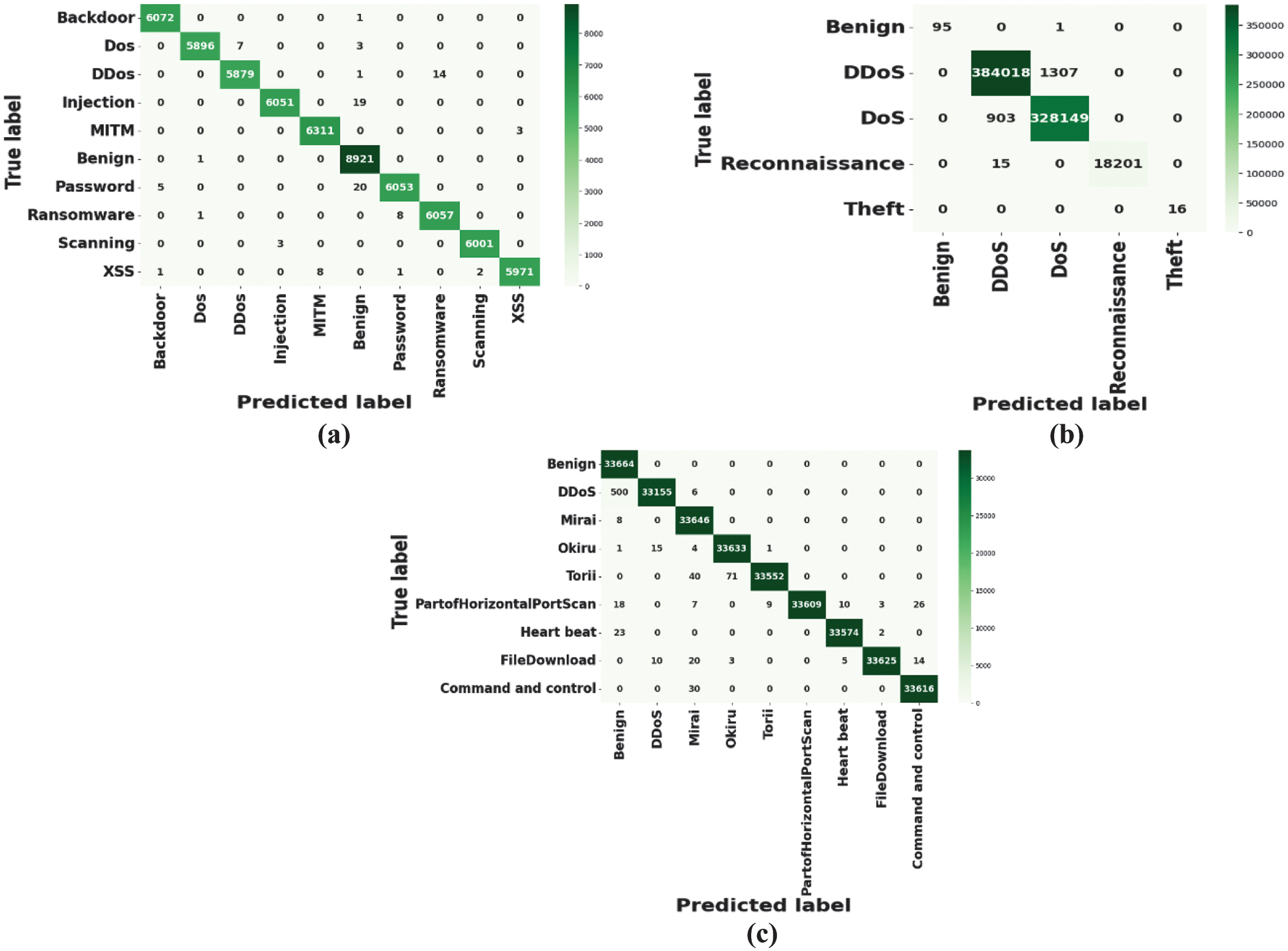 Fig. 5. Confusion matrix for the classifier on (a) ToN-IoT (b) BoT-IoT, and (c) IoT-23 datasets.
The area under the curve (AUC) in the ROC curves are exceptionally high indicating excellent discriminating ability between the attack classes and benign traffic of all the three datasets as in Fig. 6. ToN-IoT has all of the classes of AUC greater than 0.998 with Backdoor and Benign having an AUC of nearly perfect 0.9999 and 0.9995, respectively, displaying the resilience of the model to deal with a variety of types of attacks. The model retains a high detection performance of above 0.997 in the majority of the classes and a perfect AUC of Theft at a value of 1.0000, which affirms that critical threats are precisely detected in BoT-IoT. Even in IoT-23, where we have even higher heterogeneous botnet families and traffic patterns, the values of AUC turn out to be more than 0.992, thereby indicating great generalization across heterogeneous traffic patterns.
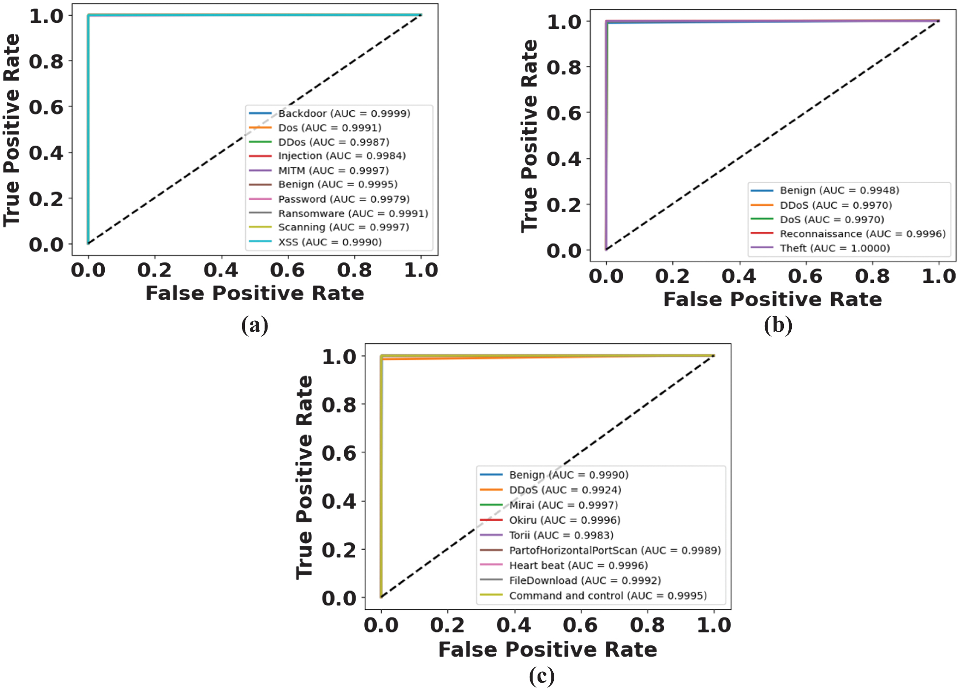 Fig. 6. ROC curve for the classifier on (a) ToN-IoT (b) BoT-IoT, and (c) IoT-23 datasets.
To analyze the model’s sensitivity to specific attack types, Table VI–VIII presents class-wise performance of the proposed LOA-BHLESNN on the Ton-IoT, BoT-IoT, and IoT-23 datasets, respectively. In this research, no new or synthetic attack types are created. The analysis is performed on the specific attack types already included in the datasets, such as Ton-IoT, BoT-IoT, and IoT-23. By reporting precision, recall, and F1-score for each of the attack classes, the model’s sensitivity and robustness against various threat types are demonstrated. Table VI illustrates the results of the suggested model on the ToN-IoT dataset on its 11 categories and recounts the precision, recall, and F1-scores, which showed fine values. The majority of the classes show above 99.7% of results across all the metrics, meaning that they are quite strong in terms of robustness in separating benign and wide varieties of attacks. Attack patterns that are related or similar, such as DDoS, DoS, injection, and XSS, are labeled with close to 100% precision. The model is displayed to have an outstanding generalization to different categories of threats. Overall, it achieves the mean recall of 99.92%, the mean precision of 99.87%, and an F1-score of 99.89% securing high-scale intrusion detection of IoT.
Table VI. Class-wise result analysis of the classifier on the ToN-IoT dataset
| Classes | Precision (%) | F1-score (%) | Recall (%) |
|---|---|---|---|
| Backdoor | 99.90 | 99.98 | 99.94 |
| Dos | 99.98 | 99.83 | 99.91 |
| DDoS | 99.81 | 99.75 | 99.78 |
| Injection | 100.00 | 99.69 | 99.84 |
| MITM | 99.95 | 99.95 | 99.95 |
| Benign | 99.46 | 99.99 | 99.73 |
| Password | 99.98 | 99.59 | 99.79 |
| Ransomware | 99.98 | 99.85 | 99.92 |
| Scanning | 99.92 | 99.95 | 99.93 |
| XSS | 99.63 | 99.80 | 99.72 |
| Average | 99.87 | 99.92 | 99.89 |
Table VII. Class-wise result analysis of the classifier on the BoT-IoT dataset
| Classes | Precision (%) | F1-score (%) | Recall (%) |
|---|---|---|---|
| Benign | 100.00 | 99.48 | 98.96 |
| DDoS | 99.76 | 99.71 | 99.66 |
| DoS | 99.60 | 99.66 | 99.73 |
| Reconnaissance | 99.80 | 99.90 | 100.00 |
| Theft | 99.96 | 99.98 | 100.00 |
| Average | 99.62 | 99.77 | 99.93 |
Table VIII. Class-wise result analysis of the classifier on the IoT-23 dataset
| Classes | Precision (%) | F1-score (%) | Recall (%) |
|---|---|---|---|
| Benign | 99.76 | 99.73 | 99.70 |
| DDoS | 99.72 | 99.69 | 99.65 |
| Mirai | 99.75 | 99.71 | 99.68 |
| Okiru | 99.74 | 99.70 | 99.66 |
| Torii | 99.73 | 99.70 | 99.67 |
| PartofHorizontalPortScan | 99.77 | 99.73 | 99.70 |
| Heart beat | 99.75 | 99.71 | 99.68 |
| FileDownload | 99.76 | 99.72 | 99.69 |
| Command and control | 99.74 | 99.70 | 99.67 |
| Average | 99.75 | 99.71 | 99.68 |
Table VII shows the results of the proposed model on the BoT-IoT dataset in five classes, which perform with an overall high precision, recall, and F1-scores. The values of classes are near or above 99.7%, which shows that the model was robust in discriminating between benign traffic and various types of attacks. Even the most similar vulnerabilities, like DDoS and DoS, are detected with almost no omission. The model exhibits better generalization abilities with little decrease in terms of performance as the threat categories change. Overall, it has an average precision of 99.62%, a recall of 99.30%, and an F1-score of 99.77%, which guarantees effective IoT intrusion detection.
Table VIII indicates that the proposed model performed well on the IoT-23 dataset across nine classes, realizing a high precision, recall, and F1-scores. The majority of classes have values of at least 99.7% which indicates that they are quite robust when differentiating benign traffic from many kinds of attacks. The related or similar attack patterns, for example, DDoS and Mirai, are detected with the accuracy of nearly 100%. The model has a high degree of generalization, and there is little variance in the results of various classes of IoT threats. Finally, it has an average precision of 99.75%, average recall of 99.68%, and F1-score of 99.71% to ensure stability in terms of intrusion detection in IoT.
A.COMPARATIVE ANALYSIS
In this context, the performance of various existing methods is compared with the proposed LOA-BHLESNN using metrics such as precision, accuracy, F1-score, and recall among ToN-IoT, BoT-IoT, and IoT-23 datasets. Here, the DPFEN-CTGAN [17], SATIDS [18], ROAST-IoT [19], CNN-based Metaverse IDS [20], and AAFSO with GA-FR-CNN [21] are considered as existing research. Compared to the above-mentioned existing methods, LOA-BHLESNN accomplishes an accuracy of 99.96%, 99.94%, and 99.81% for ToN-IoT, BoT-IoT, and IoT-23 datasets, respectively. Table IX shows the comparison for all three datasets.
Table IX. Comparison of all three datasets
| Dataset | Method | Precision (%) | Accuracy (%) | F1-score (%) | Recall (%) |
|---|---|---|---|---|---|
| ToN-IoT | DPFEN-CTGAN [ | 99.58 | 99.63 | 99.56 | NA |
| SATIDS [ | 97.3 | 96.56 | 97.35 | NA | |
| ROAST-IoT [ | NA | 99.78 | NA | NA | |
| CNN-based Metaverse IDS [ | 97.6 | 99.8 | 98.9 | 99.9 | |
| LOA-BHLESNN | 99.87 | 99.96 | 99.89 | 99.92 | |
| BoT-IoT | DPFEN-CTGAN [ | 99.47 | 99.51 | 99.45 | 99.43 |
| CNN–based Metaverse IDS [ | 99.3 | 99.8 | 99.7 | 99.9 | |
| AAFSO with GA-FR-CNN [ | 86.66 | 93.77 | 91.03 | 95.87 | |
| LOA-BHLESNN | 99.62 | 99.94 | 99.77 | 99.93 | |
| IoT-23 | DPFEN-CTGAN [ | 99.61 | 99.67 | 99.59 | 99.57 |
| ROAST-IoT [ | NA | 99.15 | NA | NA | |
| LOA-BHLESNN | 99.75 | 99.81 | 99.71 | 99.68 |
B.DISCUSSION
The drawbacks of existing research and the advantages of the proposed methods are explained in this section. The DPFEN-CTGAN [17] might not account for the possibility of attacks that target an IDS. In SATIDS [18], IoT devices have limited energy and computational resources, which creates challenges without significant resource optimization. The ROAST-IoT [19] algorithm ensures optimal classifier performance under dynamic network and attack conditions. The CNN-based Metaverse IDS [20] increased the processing latency that affects a system’s ability to perform real-time attack detection. AAFSO with GA-FR-CNN [21] relies on hyperparameter tuning, which consumes time and challenges to optimize for various network conditions. The hash encoding converts the categorical features into integer form with the assistance of a hash function. The min-max normalization is applied to standardize all the variables in a similar range. Then, the LOA is applied to select optimal features and reduce the redundant features due to the ability to explore and exploit the search space, which enhances classifier performance. The BHLESNN includes the Hebbian learning rule to increase the connection adaptively based on correlation patterns of input data, thereby improving network capability for recognizing complex attacks. Moreover, the beta function is utilized for spike encoding, which enables a better presentation of features in network traffic.
C.LIMITATIONS
The proposed LOA-BHLESNN is validated on benchmark datasets, which may not reflect the real-world IoT traffic diversity and evolving attack patterns. The LOA is computationally insensitive for high-dimensional data, and BHL requires hyperparameter tuning. Furthermore, the performance is highly resource-constrained for an IoT environment.
V.CONCLUSION
The LOA with BHLESNN is proposed in this research for IDS classification. Initially, the three IDS datasets are preprocessed by hash encoding and min-max normalization. The hash encoding converts the categorical features into integer format with the help of a hash function. The min-max normalization process is utilized to standardize every variable into the same range of values to eliminate the indicators of large scales from taking over the features of other variables. Then, LOA selects optimal features and reduces redundancy because it can explore and exploit the search space, thereby enhancing classifier performance. The usage of the beta function for spike encoding enhances temporal precision and allows a better presentation of dynamic features in network traffic. The proposed LOA-BHLESNN achieves the accuracy of 99.96%, 99.94%, and 99.81% for ToN-IoT, BoT-IoT, and IoT-23 datasets, respectively. This approach can be adopted into other domains involving sequential data such as medical diagnosis, industrial fault detection, and financial fraud detection. Future work will focus on handling concept drift through continual learning, thereby enhancing zero-day attack detection and integrating explainable AI techniques to enhance model interpretability. This will help security analysis to understand the reasoning of the detection decision and assist in identifying model biases for better performance. Additionally, it focuses on investigating the applicability and generalization ability of the model in other domains, such as 5G and edge computing environments, by cross-domain experiments, as this requires access to domain-specific datasets, preprocessing, and system adaptations to ensure reliable evaluation.
NOTATION LIST
| Normalized feature | |
| Actual feature | |
| and | Minimum and maximum number of features |
| Random number in [0, 1] | |
| and | Lower and upper bound of decision variable |
| Group of safer areas for lyrebird | |
| Best objective function | |
| New location estimated for th lyrebird according to its escaping strategy | |
| New location estimated for th lyrebird according to hiding strategy | |
| Iteration count | |
| Input | |
| Result of the initial layer | |
| Arbitrary nonlinear function | |
| Parameter of self-connective feedback gain | |
| Weights interconnect output neurons with hidden layer outputs | |
| Sigmoid function | |
| Data from input and hidden layers | |
| Output of hidden layer | |
| Symbolize learning rate | |
| Unit of time frame | |
| Membrane potential | |
| Duration of neuron spike | |
| Result of the neuron’s actual spike time | |
| Residual | |
| Network input | |
| Weight matrix | |
| Network output | |
| True positive | |
| True negative | |
| False positive | |
| False negative | |
| ML | Machine Learning |
| DoS | Denial of Service |
| DDoS | Distributed Denial of Service |
| RNN | Recurrent Neural Network |
| SNN | Spiking Neural Network |
| ESNN | Elman Spiking Neural Network |
| ROC | Receiver Operating Characteristic |
CONFLICT OF INTEREST STATEMENT
The author(s) declared no potential conflicts of interest with respect to the research, authorship, and/or publication of this article.
AUTHOR CONTRIBUTIONS
M.G.V. conducted the research and drafted the initial manuscript. A.B.J. contributed to the design of the study and performed data analysis. C.L.C. provided critical insights and technical guidance and contributed to the interpretation of results. L.C.L. assisted with validation, manuscript review, and overall supervision of the work. All authors read and approved the final version of the manuscript.