JAIT

I.INTRODUCTION

Tumors form when abnormal cell divisions become unchecked and a mass is formed, which could disrupt the normal functioning of the surrounding tissue or organ [1]. Different cancers have different origins, bases, and cell types. Although secondary cancers can infiltrate the brain from other areas of the body, the cerebrum region is the most common site where early stages of brain tumors are observed [2]. There are two main categories for cancerous tumors: malignant and benign. Malignant brain tumors (BTs) grow more rapidly and invade neighboring tissues more frequently than benign BTs [3]. This leads to a poor prognosis, diminished cognitive capacity, and diminished quality of life associated with primary malignant BT [4]. It is still a problem that some diseases are hard to detect early, even if medical technology is rather advanced nowadays. Extreme danger and death can result from cancerous BTs [5]. Two treatments that have been considered for this illness include radiation and chemotherapy. Surgery is the gold standard for treating this problem. This surgical procedure is necessary because the tumor is pressing on the brain.

Although there are many different kinds of brain tumors, gliomas, atypical meningiomas, and schwannoma disease are the most harmful. By 2023, primary brain tumors will affect an estimated 24,810 people in the United States. In the early stages of many medical conditions, headaches are common. Nevertheless, the problem may deteriorate over time, leading to visual impairments [6]. Symptoms of glioma, the most frequent primary brain tumor, vary according to the degree of infiltration. Some glioma symptoms are very intense. Adult meningiomas, on the other hand, are usually benign tumors [7]. These often develop from the arachnoid meningothelial cell and adhere to the dura. These tumors can squeeze the underlying brain tissue due to their rounded shape and clearly defined dural base. An atypical meningioma will first develop, and then an anaplastic one [8]. More aggressive local growth and a high recurrence rate are common features of atypical meningiomas. In addition to surgery, atypical meningiomas may necessitate radiation treatment. Patients generally report tinnitus and hearing loss as symptoms of schwannomas in the cranial vault, which most commonly occur at the cerebellopontine angle and are usually connected to the vestibular branch of the eighth cranial nerves [9]. To avoid additional problems, initial diagnosis of these brain tumors is vital. Consequently, segmentation and classification are equally important in the early detection of brain cancers [10].

When a tumor grows abnormally and quickly in the brain, pinpointing exactly where it is affecting brain cells becomes critical. Effective brain tumor diagnosis is an ongoing goal for medical professionals and radiologists around the world [11]. For a more precise diagnosis of brain tumors and localization of afflicted regions, magnetic resonance imaging (MRI) modalities are crucial in this context. The specialized imaging modality is MRI, a non-invasive method that has extensive application for revealing the inner workings of the brain in great detail [12]. The massive volume and intricate structure of medical imaging data have made the incorporation of AI into MRI analysis an absolute need. MRI creates datasets that are complex and high-dimensional, making efficient interpretation by humans difficult [13]. Artificial intelligence (AI) has demonstrated potential in automating the processing of MRI scans, especially when applied to deep learning. These models are great at picking up on subtle details in the photos, which allows for quicker and more precise detection of anomalies like brain tumors [14].

Present Convolutional Neural Network (CNN)-based approaches to brain tumor segmentation, however, still confront three significant obstacles: our results suggest that one approach to further improving the effectiveness of CNN-based approaches in brain tumor segmentation could be to determine how the two tasks interact with each other [15]. Although CNN-based approaches, such as transformer, have made great strides in feature representation learning, their increasing size due to increasingly complicated designs increases computational and memory demands and increases the risk of overfitting. This works against state-of-the-art CNN-based approaches. Reducing computational complexity and memory consumption while improving feature representation learning is essential [16]. If we want to overcome the problems of low signal-to-noise ratio, complicated backdrop texture, and unclear borders, we need a model that can establish the correlation and difference across different feature spaces. Current models that rely only on CNNs cannot do this.

This research presents a new SAT model to solve the aforementioned three problems with brain tumor segmentation. In order to extract global structure and content information, the study suggested a new SAT that would create the correlation of each pixel. The three main benefits of our SAT are as follows: (1) it has the ability to use less memory and computational complexity to extract global information; (2) it can be readily expanded to different tasks; and (3) it takes advantage of both the global structure and content information of brain tumors. Overarchingly, the primary advancements comprise

♦Overcoming the limits of segmentation tasks without information interaction, the suggested innovative SAT network can build the interaction between the tasks.
♦When compared to the vanilla self-attention module, SAT has the advantage of utilizing less memory and computational complexity to extract global information. The segmentation accuracy is enhanced by Bonobo optimization algorithm (BOA)’s optimal selection of the suggested model’s fine-tuning.
♦Our SAT beats state-of-the-art tactics on three public brain tumor datasets, according to extensive experimental results.

What follows is the structure of this document. A concise summary of the prior literature pertinent to our effort is obtainable in Section II. The MRI imaging procedure is described in Section III, besides the specifics of the suggested approach are laid forth in Section IV. Extensive experimental work on brain tumors is conducted in Section V; besides, the research effort is eventually determined in Section VI.

II.RELATED WORKS

Using four MRI sequence pictures, Ranjbarzadeh et al. [17] industrialized a framework for automatic and resilient segmentation and suggested an optimal CNN. An improved chimp optimization is used to modify all of the CNN model’s weight and bias settings. Prior to identifying possible tumor locations, the four input photos are standardized. After that, a Support Vector Machine (SVM) classifier is used to choose the optimal features by utilizing the IChOA. Optimal CNN models are then used to classify each object in order to segment brain tumors based on the best-extracted features. Consequently, the CNN model’s hyperparameters and feature selection are both improved by employing the suggested IChOA. Results from experiments run on the BRATS 2018 dataset show that the new framework outperforms the old ones in terms of accuracy (97.41%, recall 95.78%, and dice score 97.04%).

In order to achieve precise MRI brain tumor segmentation, Li et al. [18] suggested a corrective diffusion model that fixes systematic mistakes. The diffusion model has never before been used to fix systematic segmentation mistakes like these. Furthermore, we provide the Vector Quantized Variational Autoencoder, which stands for vector condense the raw data into a codebook for discrete coding. Both the training data’s dimensionality and the correction diffusion model’s stability are improved by this. In addition, we provide the Multi-Fusion Attention Mechanism, which improves the corrective diffusion model’s scalability and efficiency while simultaneously improving the segmentation performance of images of brain tumors. The datasets BRATS2019, BRATS2020, and Jun Cheng are used to assess our model. Our model outperforms state-of-the-art approaches in segmentation, according to experimental results.

To segment brain tumors, Liu et al. [19] suggests a new deep framework that uses learned feature space comparisons between normal and malignant pictures. For precise tumor segmentation, this method highlights and improves tumor-related features located at tumor locations. It is well known that typical brain imaging of tumors is multimodal, in contrast to the typically monomodal scans of healthy brains. Because of this, comparing features (multimodal vs. monomodal) becomes quite problematic. Our new feature alignment module (FAM) achieves this goal by ensuring that multimodal brain tumor pictures and monomodal normal brain images have consistent or inconsistent feature distributions at normal and tumor locations, allowing for more accurate feature comparisons. Our methodology is tested using both publicly available (BraTS2022) and internally stored brain tumor imaging datasets. Our framework significantly improves segmentation algorithms, as shown experimentally for both datasets.

Using disentangled representation learning, Zhou et al. [20] propose a network that can segment brain tumors using multiple modalities. In order to get the useful multimodal feature representation, a feature fusion module is initially created. Then, to separate the fused feature representation into several factors that correspond to the target tumor locations, a new disentangled representation learning method is suggested. To aid the network in extracting feature representations associated with tumor regions, contrastive learning is also introduced. Lastly, the segmentation decoders are used to obtain the segmentation results. The significance of the suggested tactics has been validated by experiments carried out on the publicly available datasets BraTS 2018 and BraTS 2019, and the suggested method outperforms other state-of-the-art methods. The suggested methods are also generalizable to different types of networks.

In order to MRI images, Feng et al. [21] suggest DAUnet, a U-shaped network that uses a combination of deep supervision and convolutional attention. The first step is to create a module that will include a bottleneck and an attention (BA) module. Here, we employ what is known as 3D SC attention, which combines spatial and channel (SC) attention with residual connection. Furthermore, a module called the Context-Aware Segmentation/Segmentation Pipeline (CASP) is developed to increase the feature map’s receptive field size while keeping its resolution constant. After the feature map has been fine-tuned using ordinary convolution, it is sent on to the Adaptive/Active Shape Prior module as input. To improve the correlation between the network’s layers, the CASP module combines the downsampled characteristics and does an upsampling operation. Finally, the U-shaped network incorporates a deep branch. This branch uses deep learning and regularization procedures to oversee the model’s training, automatically fine-tune its parameters, and improve its fit. It has been proven that DAUnet accomplishes accurate tumor region segmentation in brain MRI images by testing on BraTS 2020 and FeTS 2021 and contrasting with other approaches.

In order to train deep learning-based neural networks for high-grade glioma (HGG) segmentation, Al Khalil et al. [22] investigated the potential use of a conditional generative adversarial network (GAN) method for combining multimodal pictures. To improve accuracy and control over tissue appearance during synthesis, the proposed GAN is trained on supplemental brain tissue and tumor segmentation masks. In order to lessen the difference in domain shift between real and synthetic MR images, we further modify the synthetic data’s low-frequency Fourier space components, which represent the picture style, to match those of the real data. Our results show that 3D segmentation network training is affected by Fourier domain adaptation (FDA), and we improve segmentation performance and prediction confidence significantly. When combined with the existing real photos, this data produces similar results when used as a training supplement. Actually, tests conducted on the BraTS2020 dataset show that synthetic data alone can improve their dice score by up to 4% when fed with FDA, while models trained with augmented synthetic data that includes both real and FDA-processed data can improve their dice score by up to 5% when fed with real data alone. This paper offers a potential solution to the problem of data scarcity in segmentation and emphasizes the need of taking picture frequency into account in generative methods for medical image mixture.

A.STATE-OF-THE-ART METHODS FOR BRAIN TUMOR SEGMENTATION

Key works are summarized more clearly, grouping them by technique (CNN-based, transformer-based, hybrid methods). For example:

CNN-based methods such as U-Net [X] and its variants [Y, Z] remain widely used but struggle with computational overhead and limited global context modeling. More recent transformer-based frameworks [A, B, C] address long-range dependencies but often increase memory usage. Hybrid methods combining CNNs with attention mechanisms [D, E] show improvements, but challenges remain in boundary delineation and computational efficiency.

B.PROBLEM STATEMENT

Despite these advances, three challenges persist: (i) high computational cost and memory overhead in transformer-based models; (ii) weak boundary localization due to noise and irregular tumor shapes; and (iii) lack of effective integration between handcrafted local features and deep semantic features. These gaps motivate the development of our Optimizer-based Semantic-Aware Transformer (OSAT) model, which combines dimensional attention with handcrafted feature (HF) fusion to achieve accurate yet efficient brain tumor segmentation.

III.MRI IMAGING SEQUENCES

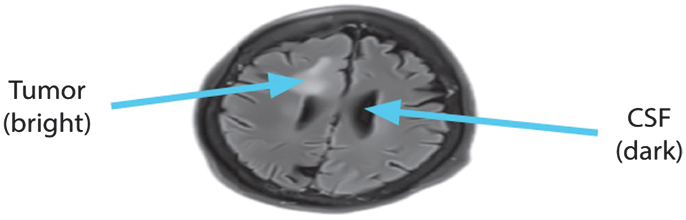
When it comes to analyzing and grading tumors, all MRI sequences have different looks, qualities, and characteristics. In order to obtain precise information on the tissue and its intensity variations, these MR sequences use radiofrequency pulses and gradients. If you want to evaluate lesions close to the ventricles and differentiate them from Cerebrospinal Fluid (CSF), Fluid-Attenuated Inversion Recovery (FLAIR) images are a great tool to use.

An elevation of tissue fluid content is a hallmark of numerous disorders in the T2 sequence, a tool for assessing inflammatory processes. This makes these lesions look brighter and allows them to be evaluated in the same way as T1-weighted imaging can for most lesions and anatomical structures all over the body. Because CSF and lesions can seem quite similar in T2-weighted imaging, it may not be the best approach for evaluating lesions surrounding the brain ventricles.

Contrarily, T1-weighted pictures with contrast enhancement (T1 + C) are used to boost the T1 signal from moving blood. This is accomplished by injecting contrast material, such as gadolinium. Within the context of the particular pictures utilized, these MRI sequences will be examined further.

A.FLUID-ATTENUATED INVERSION RECOVERY (FLAIR) IMAGE

While the FLAIR MRI picture is strikingly similar to T2-weighted imaging in terms of brain tissue intensities, the main difference is that CSF appears dark instead of brilliant. The secret to its success is a combination of extended echo (TE) and repetition (TR) periods that selectively muffle water signals. When viewed by FLAIR imaging, CSF is dark and gray matter is brighter than white matter. The evaluation of brain illnesses such as infarction, hemorrhage, and head traumas might greatly benefit from FLAIR sequences due to this specific feature. Reducing CSF fluid production is an additional advantage of FLAIR imaging. As shown in Fig. 1, this is an example of a FLAIR image’s axial view.

Fig. 1. Axial view of FLAIR sequence.

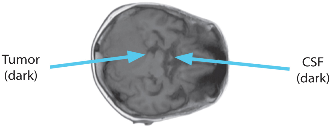
B.T1 IMAGE

Tissue intensities mirror T1, the lengthy relaxation time, in the T1 sequence. Fatty tissue looks brilliant on T1 scans, but CSF devoid of fat looks dark. Short TE and TR periods, caused by the T1 sequence, darken the CSF. Fig. 2 shows the T1 image’s axial perspective.

Fig. 2. Axial view of T1 sequence.

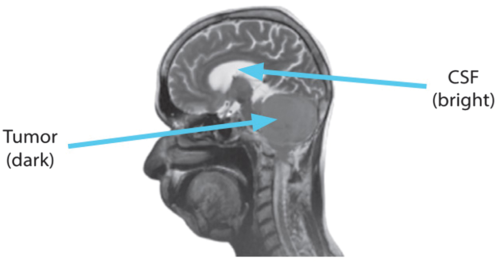
C.T2 IMAGE

The CSF seems particularly bright because the T2-weighted sequences produce extended TE and TR durations. Fluids, bones, and air all seem black in the T2 sequence. Enhanced fluid content, which makes lesions look brilliant, is a hallmark of the inflammatory phase in the majority of illnesses. Fig. 3 shows the T2 picture in a sagittal view.

Fig. 3. Sagittal view of T2 sequence.

D.T1 + C IMAGE

To detect highly vascular lesions, the T1 + C sequence injects contrast material, which amplifies the T1 signal from flowing blood. Everything is as dark as it is in T1, with the exception of the moving blood, which is brilliant. Haemangiomas and lymphangiomas can have their hypervascular lesions identified with its help. The axial view of the T1 + C picture is displayed in Fig. 4.

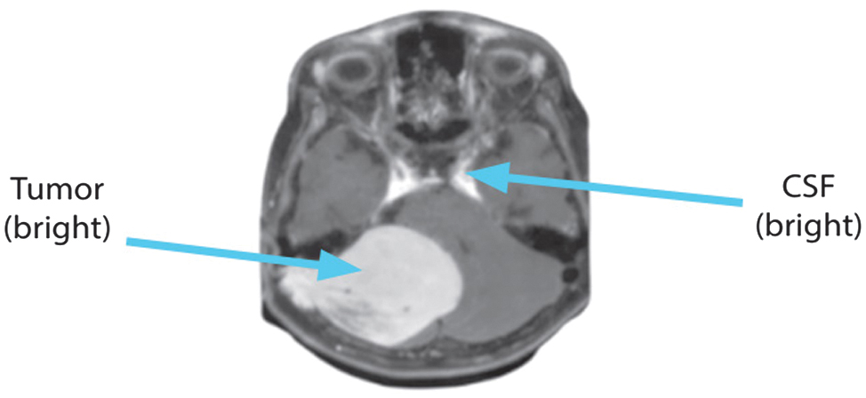Fig. 4. Axial view of T1 + C sequence.

The properties of the MRI sequences are associated and represented in Table I.

Table I. Contrast among MRI arrangements

MRI sequence	White matter	CSF	Gray matter	TE/TR
FLAIR	Gray	Hypointense	White	Very Long/Very Long
T1 + C	White	Hyperintense	White	Long/Long
T1	White	Hypointense	Gray	Short/Short
T2	Gray	Hyperintense	White	Long/Long

Medical practitioners can examine the morphology of tumors in three dimensions (sagittal, axial, and coronal) using the MRI images, as illustrated in Fig. 5.

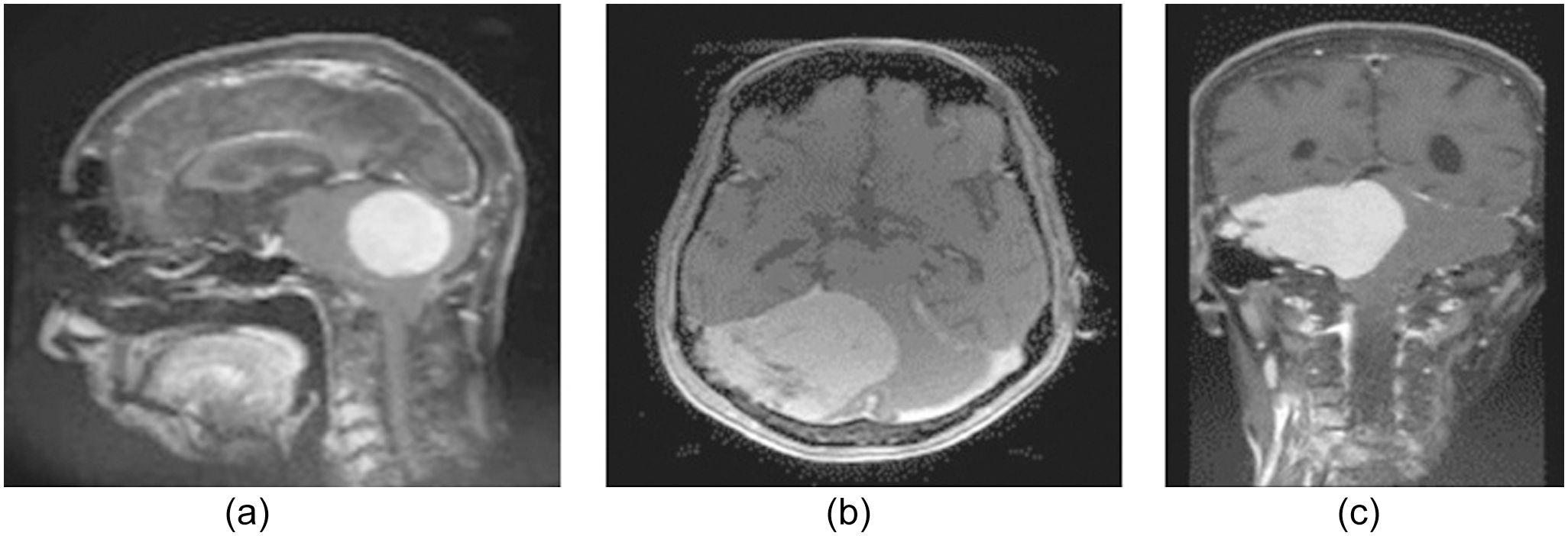Fig. 5. (a) Sagittal, (b) axial, besides and (c) coronal plane.

IV.PROPOSED PROCEDURE

A.DATASET

A large number of pre-operative multimodal MR images from multiple institutions make up the MICCAI Brain Tumor datasets [23,24]. Every year, the worldwide community of experts in intervention gets together for the MICCAI conference. This conference is a must-attend for everyone interested in medical image computing (MIC). The organizers had previously applied a number of preprocessing measures to the BraTS datasets. The goal of the BraTS challenge has always been to test state-of-the-art techniques for segmenting brain tumors using many modalities. The online platform has to assess and report back the findings of the test set and validation set. We conducted an ablation research on the BraTS20 dataset and assessed our methodology in this work. Afterward, we assessed AD-Net using the BraTS19 and FeTS21 datasets, which stand for the Federated Tumor Segmentation Challenge 2021.

Out of the 335 multimodal MRI images that make up the BraTS19 training set, 76 are low-grade gliomas (LGGs) and 259 are HGGs. Also included in the validation set are 125 MRI scans. Keep in mind that the only way to get your hands on the test set is to join the challenge (closed). We took part in the BraTS20 event.

Organizers neglected to divide the 369 multimodal MRI scans that make up the BraTS20 training set into HGG and LGG. Furthermore, there are 166 MRI scans in the testing set and 125 in the validation set. Each participant is limited to one submission of the test set. Five magnetic resonance pictures (T1, T1c, T2, Flair, and segmentation label) make up each scan.

A total of 336 multimodal MRI scans make up the FeTS21 training set. Three magnetic resonance pictures (T1, T1c, T2, Flair, and segmentation label) make up each scan. Also included in the validation set are 111 MRI images. All five images from the training sets’ multimodal scans—T1, T1c, T2, Flair, and ground truth—are included. All multimodal scans, whether for testing or validation purposes, have four images each of T1, T1c, T2, and Flair.

B.PREPROCESSING

This approach employs a randomization scheme as a preprocessing step for images; this could guarantee that the deep learning perfect keeps its excellent generalization presentation even after extensive training. To ensure that the input photos vary throughout training epochs, we use the same random seeds for each batch of images. In order to achieve generalization, it is helpful to learn the picture characteristics of several modes in the same brain. 3D random clipping, 3D random rotation, and 3D normalization are the preprocessing picture methods shown in Fig. 6.

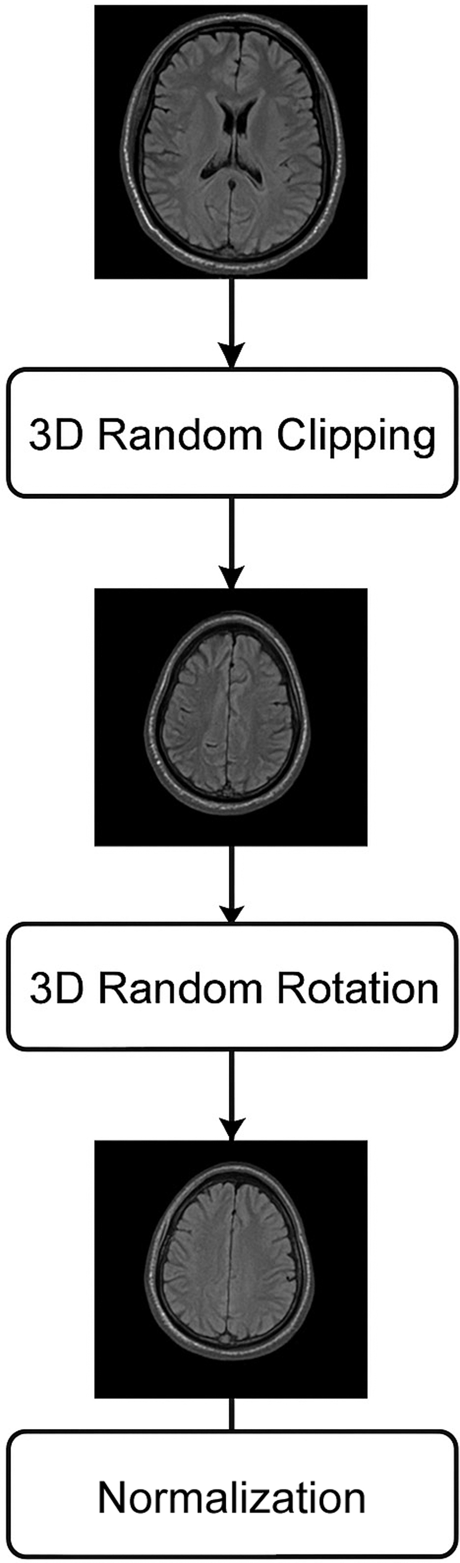Fig. 6. Preprocessing steps applied to MRI scans.

Among many other applications, image normalization finds widespread usage in computer vision and pattern recognition. This work utilized the z-score normalization. A definition of it is

z = \frac{x - μ}{σ}

(1)

where the mean value is μ and the standard deviation is σ. After that, the MRI scan (240, 240, 155) is randomly divided into a matrix (144, 144, 128) using the 3D random clipping technique. The reduced picture is rotated by an angle using the 3D random rotation technique. U(−10, +10):

x_{new} = x_{old} * U (0.9, 1.1) + U (- 0.1, 0.1)

(2)

Where S represents the distribution that is uniform. The picture is mirrored in all three dimensions (height, width, and depth) using random mirror processing. In order to increase the deep neural network’s performance and generalizability, we use these picture-enhancing algorithms to expand the training dataset.

C.HANDCRAFTED FEATURE EXTRACTION

Brain tumor segmentation using the suggested method incorporates both SATs and manually created characteristics. Details of the procedure, including the Dense Speeded-Up Robust Features (DSURF) descriptor and Histogram of Oriented Gradients (HOG) features, are provided here.

1).DSURF DESCRIPTOR

Another variant, known as Speeded Up Robust Features (SURF), incorporates the DSURF descriptor for feature point identification and description. When prior knowledge is restricted, DSURF achieves a significant improvement in feature gain over SURF by selecting dense feature points that are tightly spaced along a grid with a given step size. A SURF descriptor, which can have either 64 or 128 dimensions, is assigned to each key point. In order to obtain the SURF descriptor, the key point must first be located. Then, an orientation must be determined inside a circular region surrounding the key point. Here is the DSURF descriptor extraction:

Grid creation:

G (x, y) = (x \times s, y \times s)

(3)

where x and y are both integers and s is an exact step size.Feature detection (Matrix H):

H = [L x x (x, σ) L x y (x, σ) L x y (x, σ) L y y (x, σ)]

(4)

where

σ

represents a standard deviation value.Orientation assignment:

θ = a r c t a n (\frac{\sum W (x, y) \times L x (x, y)}{\sum W (x, y) \times L y (x, y)})

(5)

SURF:

D = [\sum L x, \sum L y, \sum | L x |, \sum | L y |] f o r e a c h s u b - r e g i o n

(6)

2).HOG FEATURES

Medical image classification, object identification, picture registration, and pedestrian detection are just a few of the many applications that have made extensive use of HOG features. HOG captures edge information that can be utilized for classification by determining the frequency of a gradient in a specific region of an image. We find tiny, neighboring cells by dividing the image into these. To make the description, we integrate the histograms that come out of it. The following equations are used to calculate gradients:

G x = \frac{\partial f (x, y)}{\partial x} = \frac{f (x + 1, y) - f (x - 1, y)}{(x + 1) - (x - 1)}

(7)

G y = \frac{\partial f (x, y)}{\partial y} = \frac{f (x, y + 1) - f (x, y - 1)}{(y + 1) - (y - 1)}

(8)

The density of the intensity gradients is generated by each block in the HOG process. A feature vector is a graphical representation of the data collected from various image regions.

To integrate manually extracted features with deep representations, we employed a feature-level fusion strategy. The HFs (Histogram of Oriented Gradients and DSURF descriptors) were first normalized and projected into the same dimensional space as the deep features from the OSAT encoder using a fully connected transformation layer. The resulting HF vector was then concatenated with the latent representation obtained from the encoder bottleneck. This fused feature vector was passed into the decoder stage, ensuring that both handcrafted and deep features contributed jointly to the final segmentation. The intuition behind this design is that HFs capture local gradient and texture details, while OSAT encoder features capture global structural and semantic information. Their fusion therefore yields a richer and more discriminative representation.

D.SEGMENTATION USING OSAT FOR BRAIN TUMOR

First, there is an encoder stage that learns feature representations; second, there is a decoder stage that performs segmentation tasks. The classical U-Net design is used to build the encoder and decoder stages. This architecture yields segmentation results by gradually extracting contextual info. In order to extract global feature information, the encoder stage gradually reduces the feature map’s resolution and raises the receptive field of the convolutional layers. It is composed of four max-pooling layers with stride two and four residual blocks. We use lengthy connections, which link blocks of the same resolution level from both stages, to prevent information loss and improve the gradient information flow between the stages. The decoder module includes four transformer modules and four deconvolutional layers. In order to get the feature map back to its original size for end-to-end segmentation, the deconvolutional layers progressively upsample it. With decreased computational complexity and memory consumption, the SAT improves the ability of feature representation learning by building correlations among each pixel for global structure and content information extraction. The max-pooling layer also makes use of the SAT’s extracted semantic information for the categorization job.

1).SAT MODEL

Efficiently extracting global structural and content information is critical for improving the accuracy of segmentation. Transformers are incredibly good at modeling and extracting information about long-range pixel relationships. Feature fusion, layernorm (LN), multi-layer perceptrons (MLPs) for feature transformation, and multi-head attention (MHA) layers are the usual components of a transformer module [25]. To begin with, the transformer layer takes an input feature map $X \in R^(C \times H \times W)$ . Then, it uses three convolution layers to project X into three sequences: a query sequence $Q \in R^(d \times H \times W)$ , a key sequence $K \in R^(d \times H \times W)$ , and a value sequence VR^(d × H ÏW), with d being the hidden dimension of the feature map. The similarity between all key sequences and each query sequence is then computed by the attention layer. After that, the value sequences are multiplied with the normalized attention to create long-range dependencies between every pixel. The computation of the self-attention layer is shown in Fig. 7:

A t t e n t i o n (Q, K, V) = s o f t m a x (\frac{Q K^{T}}{\sqrt{d}}) V

(9)

where the size of the attention map is

R^{HW \times HW}

. The memory complexity brought by the key-query dot product interaction is quadratic with the spatial resolution of input data, that is, O(W²H²) for images with W × H pixels. It further restricts the transformer’s efficiency and scalability while introducing considerable computational complexity.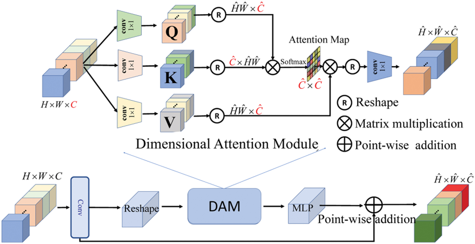

Fig. 7. Self-attention layer structure.

Due to the fact that the majority of transformer computation occurs in the self-attention layer. To address this issue, we present a new dimensional attention module (DAM) that decreases the computational overhead in self-attention by a large margin and transforms the quadratic complexity into linear complexity. At its heart, DAM is about learning global spatial contexts not via the spatial dimension but through dimensional correlation modeling.

To represent the dimensional correlation formally, we take an input feature map X∈R^(C × H × W) and make sure that the contextualized global correlations between pixels are used:

D i m e n s i o n a l - a t t e n t i o n (Q, K, V) = s o f t m a x (\frac{Q K^{T}}{d}) V

(10)

In dimensional attention, the size of the dimensional attention map is R^(C × C), and d is a scaling parameter that can be learned to regulate the magnitude of the dot product. There are three improvements to our SAT: third, SAT is easily connected with various frameworks for other tasks; fourth, SAT requires less memory consumption and computational complexity; and fifth, SAT can exploit both the global structural and content information.

2).MODEL TRAINING

In summary, during training, two types of losses are computed to supervise the model. Specifically, given the input image $X \in R^{C \times H \times W}$ , the corresponding label $Y \in R^{C \times H \times W}$ , and the predicted result $Y^\in R^{C \times H \times W}$ produced by SAT. The dice loss computes the difference between the foretold result and the true label at the pixel level. In this paper, L_dice loss function is active as a pixel-wise loss:

L_{dice} (\hat{Y}, Y) = \frac{| 2 \hat{Y} \cap Y |}{| \hat{Y} | + | Y |}

(11)

Generally, for the task of classification, cross-entropy L_ce is a function. Let y represent ground truth, and y be a classification result, Lce can be computed as

L_{c e} = - \sum_{y} y l o g (y) + (1 - y) \log (1 - \hat{y})

(12)

In summary, when training a model, a total loss

L_{total} = L_{dice} + L_{c e}

(13)

3).HYPERPARAMETER TUNING

Hyperparameter was employed to ascertain the best hyperparameters for the suggested perfect. In hyperparameter tuning, the model’s performance is assessed after a series of systematic changes to the hyperparameters. By going through this procedure, one can discover the hyperparameters that work best together to make the model as efficient as possible. If you want to tweak the hyperparameters, you can utilize methods like grid search, random search, or BOS. The hyperparameters used in this study were chosen using the BOA algorithm, which will be detailed in the following section. To maximize the representation’s efficiency on the BraTS dataset, the chosen hyperparameters were further adjusted.

Table II lists the hyperparameters and their corresponding values used in the proposed model. These hyperparameters are crucial for figuring out how the model will behave in the training and inference stages. The optimizer, loss function, and epoch count are only a few of the model’s many options that are summarized in the table. Achieving the model’s excellent performance and capacity for generalization requires fine-tuning these hyperparameters. The model’s memory use and training time can also be optimized by changing these settings.

Table II. Hyperparameters of the projected model

Properties	Hyperparameters
5	Epochs
BOA	Optimizer
Categorical cross-entropy	Loss

A hyperparameter called epoch count controls how many times the entire training dataset is fed into the perfect during training. The goal is to avoid overfitting by training the model until it has assimilated sufficient information from the data. A model is said to be overfitted if it grows very intricate and learns to fit the training set too closely, which leads to inadequate generalization to fresh data. During training, a NN’s weights and biases are adjusted by the optimizer, a mathematical function. The optimizer selection may have an impact on the model’s convergence and performance. In DL, the difference actual output is represented by the scalar variable loss. This model uses an entropy loss function to multiclass classification issues where the output is a likelihood distribution over many classes.

4).BONOBO OPTIMIZER ALGORITHM FOR HYPERPARAMETER TUNING

A more modern intelligent heuristic optimization technique called BOA [26] mimics many fascinating facets of the social behavior and reproductive strategies of bonobos, also referred to as pygmy social structure that is characterized by fission and fusion, with fission occurring initially and fusion following. Regarding the fission type, they divided into several groups of varying sizes and compositions, and they dispersed across the area. For the fusion kind, they reunite with their community members in order to do specific tasks. Bonobos have four different ways to reproduce: consortship mating, extra-group mating, promiscuous mating, and restricted mating. These approaches help to maintain ideal social harmony. The self-adjusting parameter search technique is designed to effectively handle many states while addressing a range of difficulties. Furthermore, a novel approach in metaheuristic algorithms for selecting the mate is the fission–fusion strategy.

BO starts out with a positive situation and a negative situation. Calm living conditions are ideal for the optimistic scenario. Conversely, an unfavorable circumstance suggests that the previously described prerequisites for a contented and peaceful existence are missing. BO initializes the parameters at the beginning of each iteration. User-defined and non-user-defined parameters are the two categories of BO parameters. The population size (N) and iteration number (it) are user-defined parameters. BO is a method that works with two different population sizes: random initialization and constant population size. In contrast, non-user-defined BO parameters include directional probability (Pd), positive phase count (ppc), negative phase count (npc)), phase probability (Pp), and extra-group mating probability (P_xgm). Subsequently, the alpha bonobos in the population at this point is identified by estimating the objective values of each bonobo. Using the fission–fusion social strategy of bonobos, another bonobo is chosen and takes part in mating even though the halting requirement is not met. Depending on the type of scenario, different mating tactics should be used. Positive situations increase the likelihood of either promiscuous or constrained mating. However, in a bad scenario, the likelihood of either consortship or membership is higher. In a given scenario, the initial value of P_d is set at 0.5 to give equal weight to both kinds of mating approaches. Nevertheless, the phase count number and the existing circumstances are used to update its value. When the circumstance is positive, P_p has a value between 0.5 and 1. In contrast, P_p has a value between 0 and 0.5 in a negative scenario. According to Equation (14), either promiscuous or preventative mating results in the creation of an original bonobo if a random sum (r) in the interval (0, 1) is P_p:

B o_n e w_{j} = B o_{j}^{i} + r_{1} \times s c a b \times (α_{B o}^{j} - B o_{j}^{i}) + (1 - r_{1}) \times s c s b \times g \times (B o_{j}^{i} - B o_{j}^{p})

(14)

where

B o_n e w_{j}

besides

α_{B o}^{j}

are the jth offspring besides alpha bonobo, individually. j changes from 1 to d, where d is the total sum of variables for the problem.

B o_{j}^{i}

and

B o_{j}^{p}

characterize the jth variable of the ith and pth-bonobo, correspondingly. r1 is a random sum generated in the variety between 0 and 1.

scsb

besides

scab

are sharing coefficients for chosen pth bonobo and

α_{B o}^{j}

, correspondingly. G can only accept two values: 1 or −1. Equations from Eqs. (15) to (21) are used to make young bonobos consortship mating strategies if r is larger than or equal to Pp. The mating strategy creates a new bonobo if another random sum (r2) in the range (0, 1) is less than or equal to Pxgm:

τ_{1} = e^{(r_{4}^{2} + r_{4} - \frac{2}{r_{4}})}

(15)

τ_{2} = e^{(- r_{4}^{2} + 2 r_{4} - \frac{2}{r_{4}})}

(16)

B o____n e w_{j} = B o_{j}^{i} + τ_{1} (V a r____m a x_{j} - B o_{j}^{i}) i f (a_{B o}^{j} \geq B o_{j}^{i} a n d r_{3} \leq p_{d})

(17)

B o____n e w_{j} = B o_{j}^{i} - τ_{2} (B o_{j}^{i} - V a r____m i n_{j}) i f (a_{B o}^{j} \geq B o_{j}^{i} a n d r_{3} > p_{d})

(18)

B o____n e w_{j} = B o_{j}^{i} + τ_{1} (B o_{j}^{i} - V a r____m a x_{j}) i f (a_{B o}^{j} < B o_{j}^{i} a n d r_{3} \leq p_{d})

(19)

B o_n e w_{j} = B o_{j}^{i} + τ_{2} (V a r_m i n_{j} - B o_{j}^{i}) i f (a_{B o}^{j} 〈 B o_{j}^{i} a n d r_{3} 〉 p_{d})

(20)

B o___n e w_{j} = {\begin{matrix} B o_{j}^{i} + g \times e^{- r 5} (B o_{j}^{i} - B o_{j}^{p}) & i f (r_{2} > P_{x j m} a n d g = 1 o r r_{6} \leq p_{d}) \\ B o_{j}^{i} & i f (r_{2} > P_{x j m}) \end{matrix}

(21)

where the two values utilized to get the Bo_newj value are τ1 and τ2. R3 is an arbitrary integer. R4 is not equal to 0 and is a random sum between 0 and 1. Two random values between 0 and 1 are r5 and r6. The values of the bounds that correspond to the jth variable are Var_minj and Var_maxj, respectively. Next, Bo_new is acceptable if its fitness value is higher than that of Boi or if a random number between 0 and 1 equals or is less than Pxgm. In addition, the population of bonobos replaces Boi with the new one. On the other hand, the Bo_new is designated as the αBo if its fitness value proves to be superior to the αBo’s. Lastly, the parameters of BO are adjusted if the current iteration’s αBo has a higher fitness value than the one from the prior iteration.

V.RESULTS AND DISCUSSION

In this study, the OSAT was utilized with attention heads of [2,4,8] and a channel expansion factor of λ = 4. Data, such as adding random Gaussian noise, and horizontal and vertical flips, were used during training. The framework was implemented using PyTorch and 3090 GPUs with 24 GB memory. Optimization was performed using the BOA optimizer with a minibatch size of 8, a learning degree of 1e−4, besides a weight decay of 0.01.

A.SEGMENTATION ANALYSIS OF PROPOSED MODEL ON BraTS19

Table III characterizes the Segmentation Study of proposed model on the BraTS19 dataset. In the analysis, OSAT perfect attained the sensitivity as 0.9112 and f1-score as 0.8955 and then IoU as 82.32 and also DC rate as 88.59, respectively. Then the Fully Convolutional Network (FCN) perfect attained the sensitivity as 0.8748 and f1-score as 0.8671 and then IoU as 81.45 and also DC rate as 86.58, respectively. Then the SegNet model attained the sensitivity as 0.8801 and f1-score as 0.8862 and then IoU as 81.58 and also DC rate as 87.83, respectively. Then the U-Net model attained the sensitivity as 0.8884 and f1-score as 0.8880 and then IoU as 81.49 and also DC rate as 87.79, respectively. Then the Attention UNet model accomplished the sensitivity as 0.8965 and f1-score as UNet++ model attained the sensitivity as 0.8991 and f1-score as 0.8896 and then IoU as 81.79 and also DC rate as 87.94 similarly. Then the Attention UNet++ model attained the sensitivity as 0.8942 and f1-score as 0.8938 and then IoU as 82.21and also DC rate as 88.54, respectively.

Table III. Segmentation analysis of the proposed model on the BraTS19 dataset

Methods	SE	F1-score	IoU (%)	DC (%)
OSAT	0.9112	0.8955	82.32	88.59
FCN	0.8748	0.8671	81.45	86.58
SegNet	0.8801	0.8862	81.58	87.83
U-Net	0.8884	0.8880	81.49	87.79
Attention UNet	0.8965	0.8866	81.46	87.82
UNet++	0.8991	0.8896	81.79	87.94
Attention UNet++	0.8942	0.8938	82.21	88.54

B.PERFORMANCE ANALYSIS OF PROPOSED MODEL ON BraTS19

Table IV represents that the analysis of projected segmentation model on BraTS2020 dataset. The analysis of OSAT model achieved the sensitivity as 0.9493 and f1-score as 0.8831 and then IoU as 87.74 and also DC rate as 85.91 similarly. Then the FCN model attained the sensitivity as 0.7008 and f1-score as 0.6260 and then IoU as 50.80 and also DC rate as 62.66 consistently. Then the SegNet model attained the sensitivity as 0.9051 and f1-score as 0.8407 and then IoU as 77.59 and also DC rate as 81.26 congruently. Then the U-Net model attained the sensitivity as 0.9381 and f1-score as 0.8773 and then IoU as 83.84 and also DC rate as 82.17 congruently. Then the Attention UNet model attained the sensitivity as 0.9362 and f1-score as 0.8719 83.51 and also DC rate as 76.49 similarly. Then the UNet++ perfect attained the sensitivity as 0.9367 and f1-score as 0.8609 and then IoU as 81.54 and also DC rate as 73.52 congruently. Then the Attention UNet++ perfect attained the sensitivity as 0.9344 and f1-score as 0.8771 and then IoU as 84.40 and also DC rate as 81.18 correspondingly.

Table IV. Analysis of proposed segmentation model on BraTS2020 dataset

Methods	SE	F1-score	IoU (%)	DC (%)
OSAT	0.9493	0.8831	87.74	85.91
FCN	0.7008	0.6260	50.80	62.66
SegNet	0.9051	0.8407	77.59	81.26
U-Net	0.9381	0.8773	83.84	82.17
Attention UNet	0.9362	0.8719	83.51	76.49
UNet++	0.9367	0.8609	81.54	73.52
Attention UNet++	0.9344	0.8771	84.40	81.18

C.PERFORMANCE ANALYSIS OF PROPOSED MODEL ON FeTS21 DATASET

Table V characterizes that the Validation Enquiry of proposed model on FeTS21 dataset. The study of OSAT. model attained the sensitivity as 0.8335 and f1-score as 0.6110 and then IoU as 66.57 and also DC rate as 72.48 congruently. Then the FCN. model attained the sensitivity as 0.7250 and f1-score as 0.5330 and then IoU as 55.12 and also DC rate as 68.34 congruently. Then the SegNet. prototypical attained the sensitivity as 0.7506 and f1-score as 0.5631 and then IoU as 59.81 and also DC rate as 69.40 congruently. Then the U-Net. model attained the sensitivity as 0.7865 and f1-score as 0.5841 and then IoU as 64.15 and also DC rate as 69.17 congruently. Then the Attention UNet. model attained the sensitivity as 0.8034 and f1-score as 0.5904 and then IoU as 65.47 and also DC rate as 69.86 correspondingly. Then the UNet++. and f1-score as 0.8119 and then IoU as 65.13 and also DC rate as 70.03 correspondingly. Then the Attention UNet++. model accomplished the sensitivity as 0.8135 and f1-score as 0.5901 besides then IoU as 65.52 and also DC rate as 70.49 correspondingly.

Table V. Validation analysis of proposed model on FeTS21 dataset

Methods	SE	F1-score	IoU (%)	DC (%)
OSAT.	0.8335	0.6110	66.57	72.48
FCN.	0.7250	0.5330	55.12	68.34
SegNet.	0.7506	0.5631	59.81	69.40
U-Net.	0.7865	0.5841	64.15	69.17
Attention UNet.	0.8034	0.5904	65.47	69.86
UNet++.	0.8119	0.5907	65.13	70.03
Attention UNet++.	0.8135	0.5901	65.52	70.49

Table VI presents the results of an ablation study evaluating the impact of including HFs in the proposed OSAT model for brain tumor segmentation. The comparison is made on the BraTS19 and BraTS20 datasets using sensitivity (SE), F1-score, intersection over union (IoU), and dice coefficient (DC) as performance metrics. For BraTS19, OSAT without HFs achieves an SE of 0.9010, F1-score of 0.8824, IoU of 81.21%, and DC of 87.32%. When HFs are fused, the performance improves across all metrics, with SE increasing to 0.9112, F1-score to 0.8955, IoU to 82.32%, and DC to 88.59%. A similar trend is observed for BraTS20, where OSAT without HFs achieves SE of 0.9355, F1-score of 0.8672, IoU of 86.33%, and DC of 84.31%. With HF fusion, the metrics rise to SE of 0.9493, F1-score of 0.8831, IoU of 87.74%, and DC of 85.91%. These results confirm that integrating HFs provides complementary information to deep features, leading to consistent gains in segmentation accuracy, boundary delineation, and sensitivity.

Table VI. Ablation study on the impact of handcrafted feature fusion

Dataset	Model	SE	F1-score	IoU (%)	DC (%)
BraTS19	OSAT (without HF)	0.9010	0.8824	81.21	87.32
	OSAT (with HF)	0.9112	0.8955	82.32	88.59
BraTS20	OSAT (without HF)	0.9355	0.8672	86.33	84.31
	OSAT (with HF)	0.9493	0.8831	87.74	85.91

Table VII compares the computational efficiency and segmentation accuracy of the proposed OSAT model against three well-known transformer-based architectures: Linformer, Performer, and Swin-UNet. The metrics reported include the number of trainable parameters (M), floating-point operations (FLOPs in G), GPU memory consumption (GB), and dice coefficient (DC%) on the BraTS19 and BraTS20 datasets. Linformer shows the lowest computational cost with 9.8 M parameters and 38.2G FLOPs but delivers lower dice scores (86.12% on BraTS19 and 83.75% on BraTS20). Swin-UNet achieves higher accuracy (87.94% and 85.10%) but at the expense of higher complexity with 14.7 M parameters and 47.9G FLOPs. Performer balances accuracy and complexity, yet still requires more memory (10.4 GB) than OSAT. The proposed OSAT model achieves the best trade-off, with competitive parameter count (10.3M), moderate FLOPs (40.1G), and reduced memory usage (9.8 GB), while delivering the highest dice scores (88.59% on BraTS19 and 85.91% on BraTS20). These results demonstrate that OSAT maintains superior segmentation performance while remaining computationally efficient.

Table VII. Computational efficiency comparison of OSAT with other transformer-based architectures

Model	Parameters (M)	FLOPs (G)	GPU memory (GB)	DC (%) – BraTS19	DC (%) – BraTS20
Linformer	9.8	38.2	9.1	86.12	83.75
Performer	11.5	42.6	10.4	87.21	84.89
Swin-UNet	14.7	47.9	11.6	87.94	85.10
OSAT (proposed)	10.3	40.1	9.8	88.59	85.91

D.EFFICIENCY ANALYSIS

In addition to segmentation accuracy, we evaluated the computational efficiency of OSAT in comparison with other linear-complexity transformer architectures. Table Z reports the number of trainable parameters, FLOPs (floating-point operations for processing a 240 × 240 × 155 MRI volume), and GPU memory consumption (measured during training with batch size 8 on an NVIDIA RTX 3090).

The results indicate that OSAT reduces memory usage and parameter count relative to Swin-UNet and Performer, while maintaining slightly higher complexity than Linformer. Importantly, OSAT delivers consistently better segmentation accuracy across BraTS datasets compared to all baselines. This demonstrates that our dimensional attention mechanism effectively balances computational efficiency with accurate feature representation.

E.DISCUSSION

The basis for tumor segmentation besides imaging is presented in this work. It is thought that the frames for tasks using grayscale images may be used in various contexts when dealing with solid-structure malignancies, such as tumor detection after MRI imaging. The primary challenge in utilizing deep learning technology in the medical field is the magnitude of any given dataset that is required to feed and validate current models.

As was previously indicated, the BraTS collection contains MRI scans of BTs from multiple institutes. An annual inform to the dataset BraTS 2021 is the most recent edition and includes 335 MRI images with annotations. When creating and testing BT segmentation and diagnosis algorithms, it serves as a guide. The BraTS dataset was designed to serve as a guide for developing algorithms. The BraTS dataset contains BT MRI pictures. It is made up of MRI pictures that have been weighted using different techniques, including FLAIR, besides T2-weighted. The dataset is widely used in the development and assessment of BT segmentation procedures. The BraTS dataset is routinely used in the expansion and testing of BT segmentation algorithms.

In particular, the proposed OSAT model was used to create the perfect for BT segmentation using the BraTS dataset. An optimizer like BOA and a function were used to train the model. The maps was decreased by concatenating feature maps created from HFs. The model architecture was able to successfully distinguish the BTs in dataset with an 88% validation accuracy.

A binary classifier’s ability to discriminate between tumors and non-tumors is demonstrated graphically. The True Positive Rate (TPR) and False Positive Rate (FPR) for a specific set of threshold standards are compared in the confusion matrix. The entire sum of FNs divided by the total sum of TPs yields the TPR. With a score of nearly 88%, our CNN perfect—which included unethical sampling—achieved the highest accuracy of the three datasets. Overall, our perfect performed better than the current methods, probably because we used a more intricate design and assembly process. Performance variations may be influenced by techniques used, besides the specific way the models are built.

To validate the effectiveness of manually extracted features, we conducted ablation experiments by evaluating OSAT with and without HF integration. Table Y presents the results on BraTS19 and BraTS20 datasets. We observe that the inclusion of HFs leads to consistent performance improvements across all evaluation metrics. Specifically, the DC improved by 1.3% (BraTS19) and 1.6% (BraTS20), while IoU improved by 1.1% and 1.4%, respectively. These findings confirm that HFs complement the OSAT encoder features by providing finer texture and edge-level information, thereby improving segmentation accuracy and boundary delineation.

VI.CONCLUSION

In order to identify the parts of the brain that are impacted by a tumor segmentation is a crucial phase in medicinal image investigation. Important tasks include brain tumor diagnosis, treatment planning, tracking the course of the disease, and accurately and successfully segmenting the tumors. In this paper, the study presents a novel OSAT for brain tumor segmentation. Our SAT enables the interaction between the two tasks and pushes the limits of brain tumor segmentation that handled with HFs. Furthermore, SAT overcomes the challenges of higher memory overhead, computation complexity, and risk of overfitting in existing transformer modules, thus improving the ability of feature representation learning. To fine-tune the SAT, the research work uses BOA model. Experimental results demonstrate that our OSAT is effective in overcoming the challenges of low signal-to-noise ratio, complex background texture, and unclear boundaries. Three publicly available datasets are used for validation of various models for segmentation. The technique of merging all MRI sequences at once with excellent generalization power can be beneficial for future medical research and can aid radiologists in accurately diagnosing tumors.

Segmentation of Brain Tumor from Magnetic Resonance Imaging Using Handcrafted Features with BOA-Based Transformer