JAIT

I.INTRODUCTION

Recently, the critical role played in digital worlds is software that integrates systems applications into complex system. The increasingly crucial issue is software efficiency, security, and reliability. Software defects lead to system failures, data breaches, and severe performance degradation. To deliver high-quality software products, it is essential to address and identify them early in the development cycle.

A.SOFTWARE AND ITS VULNERABILITIES

A group of applications, processes, and routines is called software, which cooperates with a computer to perform a specific task [1]. Complex machine learning applications and computationally intensive tasks are simplified by essential factors [2]. Software structures are constructed using numerous programming languages, frameworks, and tools, and they are designed to meet specific practical and non-practical necessities [3]. Software, like many complex devices, is vulnerable to errors or flaws that might compromise its reliability, overall performance, and security [4]. Any anomaly or flaw in a software that causes it to function differently than predicted is considered a software fault [5]. Human mistakes at some stage of the improvement process, poor testing, and a lack of resources are just a few of the causes of these flaws [6]. These flaws can be due to quite several factors, including poor testing, human errors during development, and a lack of funding [7]. They fall into one among four classes, such as usability flaws, security vulnerabilities, performance issues, or intentional mistakes. To guarantee software program quality and user pleasure, those flaws must be found, fixed, and avoided [8].

B.ROLE OF SDP AND CLASSIFICATION

Software defect prediction (SDP) is a procedure used to identify potential flaws in software programs before they seriously impair performance or fail to meet expectations [9]. Defect prediction and classification aim to determine the probability that particular software components have flaws so that the development team can concentrate their testing and debugging efforts on high-risk areas [10]. Teams can improve software quality and lower development costs by prioritizing testing efforts and allocating resources wisely when software problems are predicted early in the development lifecycle [11]. Software release risks are minimized through defect prediction. Before deployment, ensure problems are identified [12]. Additionally, SDP improves the overall efficiency of the software lifecycle by reducing the time spent on post-release maintenance [13]. Traditional debugging and testing techniques are frequently inadequate due to the growing complexity and scope of contemporary software systems [14].

Defect prediction is therefore essential to improving software application performance, security, and reliability. Based on software metrics and historical data, software components and defects are categorized using SDP [15]. More effective and targeted interventions are enabled by effective classification. An expensive post-deployment issue lowers the possibility of offering reliable applications [16].

C.CHALLENGES AND THE PROPOSED HYBRID APPROACH

To guarantee dependability and software quality, an essential is SDP, which addresses the issues of ineffective optimization strategies and unbalanced datasets. Because of the existing methods, the predictive performance is generally unsatisfactory, especially when handling sparse data and noisy data. To balance the data, a strong SDP model is required; it maximizes forecasting accuracy and software defect pattern identification. The variational autoencoder (VAE) model performs superiorly by leveraging important defect-inducing properties and structured latent representations. Both particle swarm optimization (PSO) and the crayfish bobcat optimization algorithm (CBOA) are combined to enhance predictive performance. Based on adaptive undersampling, the class imbalance resolves to guarantee the balanced datasets.

D.MAJOR CONTRIBUTIONS

•The learning-to-rank under-sampling (LTRUS) model uses rank, which enhances performance by improving class balance and neglecting the majority of irrelevant class instances.
•The better generalization is ensured, and the meaningful latent representations are captured using the VAE, along with intricate defect patterns.
•Search diversity enhancement and premature convergence prevention are achieved using the proposed hybrid CBOA to optimize the VAE.
•The defect classification is adjusted, and undersampling iteration limits and ratios are dynamically adjusted via a combination of PSO and CBOA. An accurate SDP and reliable results are resultant with the exploration and exploitation balances of the proposed framework.
•An effective defect categorization is enabled using the proposed scalable graph relearn attention network (SGRAN). The proposed SGRAN is introduced for effective defect classification. It combines graph-structured relearning and attention-based feature enhancement to improve consistency and accuracy. By leveraging both temporal stability and hierarchical attention, SGRAN ensures precise classification of defective modules across diverse defect types.

Organization: The existing SDP models are summarized in Section II, followed by the proposed work design which is delineated in Section III. Experimental analysis and discussions are handled in Section IV, and Section V concludes the paper.

II.LITERATURE SURVEY

Various previously created models predicting software defects and their classification are listed.

In 2024, Q. Zhang et al. [17] introduced an SDP approach using a deep Q-learning network (DQN)-based feature extraction method to improve classification performance. By eliminating irrelevant and redundant features, the approach improves interpretability and generalization. For feature selection, weight ranking and relation matrix constructions are used after a balanced sampling technique. When compared to current methods, the method achieves superior predictive accuracy and effectiveness.

In 2025, R. G. Huassain et al. [18] propose a new framework for automating the prediction of software flaws that focuses on eight distinct defect classes: LINKER, SIGFPE, NZEC, LOGICAL, SYNTAX, SIGSEGV, SIGABRT, and SEMANTIC. A specialized dataset with nine classes, eight of which contain common programming faults and one class that is error-free, was used. Finding flaws in code snippets is intended to improve software testing and development procedures. The suggested framework optimizes model hyperparameters to attain higher accuracy in defect prediction using a CodeBERT-based approach.

In 2025, J. Sararireh et al. [19] introduced a binary white shark optimizer (WSO) to enhance ensemble learning models for SDP. To increase classification accuracy, the method maximizes the number of weak learners in an ensemble. The technique improves model stability and cross-dataset generalization by honing ensemble learning.

In 2024, S. S. S. Mishra and S. K. Barisal [20] proposed an approach to software defect classification that uses supervised Machine Learning (ML) techniques to automate and improve the accuracy of bug categorization. The system employs algorithms such as decision trees, random forests, and artificial neural networks (ANNs), trained on labeled datasets with attributes such as test day, number of faults, and fault classes. These datasets are split into training and evaluation sets to build and validate the models.

In 2025, A. L. Alem et al. [21] explored a deep learning-based method for multi-label software requirement smell categorization that combines word embeddings such as ELMo and Word2Vec with sophisticated neural network architectures such as long short-term memory (LSTM), Bidirectional Long Short-Term Memory (Bi-LSTM), and Gated Recurrent Unit (GRU).

In 2025, S. Mostafa et al. [22] proposed an approach to software defect classification that emphasizes improving prediction accuracy through feature transformation. It involves extracting features from software artifacts and applying a genetic algorithm to compute a weighted transformation that better separates buggy from non-buggy instances in a lower-dimensional space. Predictive models are then trained on the transformed dataset.

In 2025, Y. Tang et al. [23] introduced a metric-based oversampling method using instance gravity to address class imbalance in software defect datasets. The technique aids in the formation of instance groups by introducing a new metric, instance gravity, to measure instance similarity. By assigning weights based on their gravity, defective instances are synthesized.

In 2025, C. Shelke et al. [24] discussed the importance of software fault prediction in improving testing efficiency and software quality. The main goal is to use classification techniques to analyze coding features and other attributes to predict software defects. The need for improved executive models to enhance fault detection accuracy is highlighted. A recent work comparison analysis is presented in Table I.

Table I. Recent work comparative analysis

Author’s	Focus	Techniques	Advantages	Limitations
Q. Zhang et al. [17]	SDP using deep Q-learning	DQN	Improves accuracy by automating feature extraction and identifying defects	Requires large datasets and is hard to interpret
R. G. Hussain et al. [18]	Multiclass software defect classification	Feedforward neural network (FNN)	Leverages pretrained language models for better defect context understanding	Model size and training time can be large; needs large labeled datasets
J. Sararireh et al. [19]	Adaptive ensemble learning for defect classification	CNN	Adapts well to changing data and improves accuracy	Risk of overfitting with imbalanced data
S. S. S. Mishra and S.K. Barisal [20]	Software bug classification	ANN	Simplicity, easy implementation, and interpretation	Lower accuracy compared to deep learning approaches
A. L. Alem et al. [21]	Multi-label classification of software requirement smells	Long short-term memory (LSTM)	Addresses multi-label nature of software smells	Requires high-quality annotated data and can be resource-intensive
S. Mostafa et al. [22]	Feature transformation for bug detection and commit classification	ANN	Enhances defect detection accuracy with refined features	Feature engineering is manual and dataset-dependent
Y. Tang et al. [23]	Imbalanced data handling in defect prediction	Generative adversarial networks (GAN)	Improves classifier performance on minority class	May introduce noise if oversampling is excessive
C. Shelke et al. [24]	Optimized ML techniques for fault prediction	CNN	Optimizes accuracy and reduces false positives.	Needs careful feature selection and struggles with noisy data.

A.PROBLEM STATEMENT

SDP and classification aim to proactively identify defect-prone components in software systems to improve software quality and maintenance efficiency. However, this task is challenged by several significant limitations, including the reliance on large, well-labeled datasets that are often difficult and costly to obtain. The overfitted and biased model leads to class imbalance. In real-world scenarios, the practical usability is reduced, and interpretability is lacking. The modeling process is complicated by noisy data and sensitivity to hyperparameter tuning.

The software structures have evolved, and it struggles with current SDP models, making it more complex. The imbalance data is limited and needs a more interpretable and robust prediction model.

III.PROPOSED METHODOLOGY

Input data are collected from five benchmark datasets and preprocessd, including missing value imputation and normalization. The LTRUS can handle class imbalance using undersampling techniques, preserving feature distributions while neglecting relevant majority-class instances. To improve defect prediction, an instance selection method is optimized using differential evolution (DE). The probabilistic modeling captures latent defect patterns, and the VAE with SDP uses refined datasets. The global exploration of BOA and structured local search of COA combined to form a novel CBOA to enhance training, thereby avoiding premature convergence. The proposed SGRAN effectively classifies the defective samples. This methodology effectively addresses class imbalance, overfitting, and interpretability issues in SDP, ensuring reliable software quality assurance. The two distinct levels of software fault behavior are represented by using functional errors and bugs. Implementation or logical-level faults are referred to as functional errors, where an incorrect deviation or functionality from the expected behavior is caused. Defect manifestations or runtime anomalies are referred to as functional bugs. During compilation, the errors are indeed resolved and detected, including syntax errors. The syntax-level issues may still arise during automated code generation, version control merging, and integration in certain large-scale compiled systems. A diagrammatic illustration of the proposed methodology is exposed in Fig. 1.

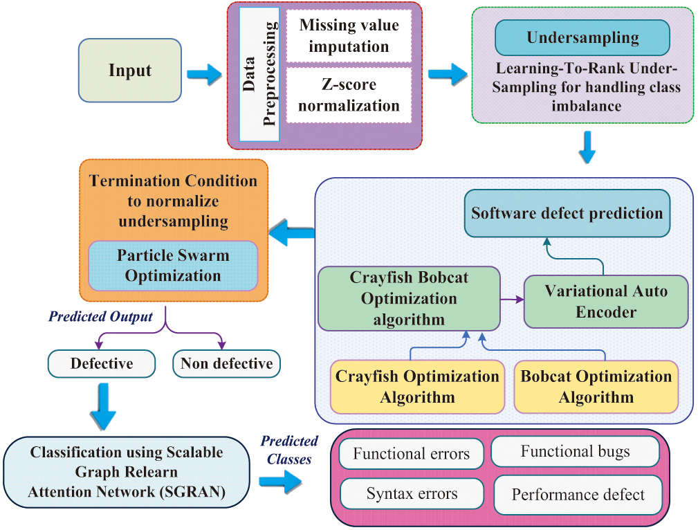Fig. 1. Schematic representation of the proposed methodology.

A.DATA COLLECTION

The input data are collected from the AEEEM, ReLink, PROMISE, SOFTLAB, and NASA repositories. The dataset $D$ is considered having $i$ data on software defects, which can be given by

D = S_{1}, S_{2}, …, S_{h}, …, S_{i}

(1)

where

S_{h}

denotes the input data and

i

denotes the total number of data items.

B.DATA PREPROCESSING

After data collection, the data undergo missing value imputation to address any incomplete entries, ensuring the dataset is complete and accurate. Z-score normalization is then applied to standardize the data, making all features comparable by removing scale differences. These preprocessing phases help to enhance the excellence and consistency of the data before further analysis. The input data $S_{h}$ is employed as the preprocessing input.

1).MISSING VALUE IMPUTATION

Missing value imputation [25] is the process of filling in missing or incomplete data with estimated values based on observed data. More reliable analysis, reduced bias, and maintained data integrity are achieved. To underline the data pattern, the relationships among the variables are preserved.

2).Z-Score Normalization

The zero mean and standard deviation for each feature are transformed and standardized using Z-score standardization. The data are normally distributed, and performance is enhanced with Z-score normalization [26]. The accuracy is improved, and the faster convergence is accomplished. The following expression represents the Z-score normalization:

g (y) = \frac{1}{σ \sqrt{2 π}} f^{- \frac{{(y - μ)}^{2}}{2 σ^{2}}}

(2)

where the feature mean, standard deviation, variables, natural logarithm base, and constant pi are described as

μ

σ

y

f

, and

π

. Hence, the preprocessed data

N_{p}

is subjected to undersampling.

3).UNDERSAMPLING

The LTRUS [27] approach aims to enhance the performance of SDP models by effectively handling class imbalance. LTRUS ranks the majority class (non-defective modules) instances by their relevance to prediction performance and removes less relevant ones, thereby improving the dataset’s overall balance. The goal is to optimize the termination condition to achieve an ideal trade-off between data reduction and predictive accuracy.

i)Generate Candidate SolutionsIn LTRUS, the DE algorithm initializes $M$ random vectors $B_{j}^{(H)}$ at generation $H = 0$ , forming a candidate solution population. Each vector $B_{j}^{(H)}$ has dimension $e$ , matching $Y$ , and is bounded by predefined limits:
$B_{\max}^{(H)} = (α_{\max, 1}^{(H)}, α_{\max, 2}^{(H)}, …, α_{\max, d}^{(H)})$ (3)
$B_{\min}^{(H)} = (α_{\min, 1}^{(H)}, α_{\min, 2}^{(H)}, …, α_{\min, d}^{(H)})$ (4)
Each feature is initialized as:
$α_{j, k}^{(H)} = α_{\min, k}^{(H)} + r a n d * (α_{\max, k}^{(H)} - α_{\min, e}^{(H)})$ (5)
where $H$ and $rand$ are the current generation and random number to [0, 1] intervals.
ii)Operate on the PopulationThe mutation operation is performed on the vectors to enhance population diversity. The mutation can be
$W_{j}^{(H + 1)} = B_{s 1}^{(H)} + G * (B_{s 2}^{(H)} - B_{s 3}^{(H)})$ (6)
where $B_{s 1}^{(H)}$ , $B_{s 2}^{(H)}$ , and $B_{s 3}^{(H)}$ are randomly chosen vectors and $G$ denotes the scaling factor. Crossover then creates a trial vector:
$V_{j}^{(H + 1)} = (v_{j, 1}^{(H + 1)}, v_{j, 2}^{(H + 1)}, … ., v_{j, e}^{(H + 1)})$ (7)
Each feature $v_{j, 1}^{(H + 1)}$ is determined as
$v_{j, 1}^{(H + 1)} = {\begin{matrix} w_{j, k}^{(H + 1)}, & i f r a n d (k) \leq C R o r k = r n b r (j) \\ α_{j, k}^{(H)}, & otherwise \end{matrix}$ (8)
where $C R$ refers to the crossover rate, $r a n d (k)$ denotes the random values in [0,1], and $r n b r (j)$ selects a feature to ensure mutation.
iii)Final Solution SelectionIf the trial vector $V_{j}^{(H + 1)}$ outperforms $B_{j}^{(H)}$ , it is replaced $B_{j}^{(H)}$ as the new candidate for the next generation. Once DE converges, LTRUS selects the best-performing candidate $B$ as the final solution, and the model $f (Y)$ is built.
iv)Handling Imbalanced DatasetsThe imbalanced dataset is processed by feeding majority class instances into the model $f (Y)$ , which ranks them based on its outputs. The lowest-ranked majority instances are then removed until the dataset achieves balance. After removal, the remaining majority instances, along with all minority instances, are used to train classifiers. Importantly, $f (Y)$ is used only for ranking and does not serve as the final prediction model. Additionally, the feature values of the majority class instances remain unchanged throughout the process. Using this method ensures a balanced dataset without changing the feature distribution. Improved model performance is classified, and SDP is subjected to the sampling data $U_{d}$ .

D.SOFTWARE DEFECT PREDICTION

The VAE performs SDP, and the connections among software metrics are captured to improve the detection of defects. The meaningful defect patterns are preserved, and the VAE learns the structured latent relationships. Smooth interpolation is maintained, and also an improved generalization is achieved. The integration of COA and BOA, called hybrid CBOA, is suggested to optimize the training of VAE. The structured local search of COA is provided, and the global exploration is enhanced using COA, thereby avoiding premature convergence. The proposed CBOA describes enhanced predictive accuracy, faster convergence, and better parameter tuning. A more reliable and efficient software defect system is enabled by the proposed VAE and CBOA.

VAE for prediction

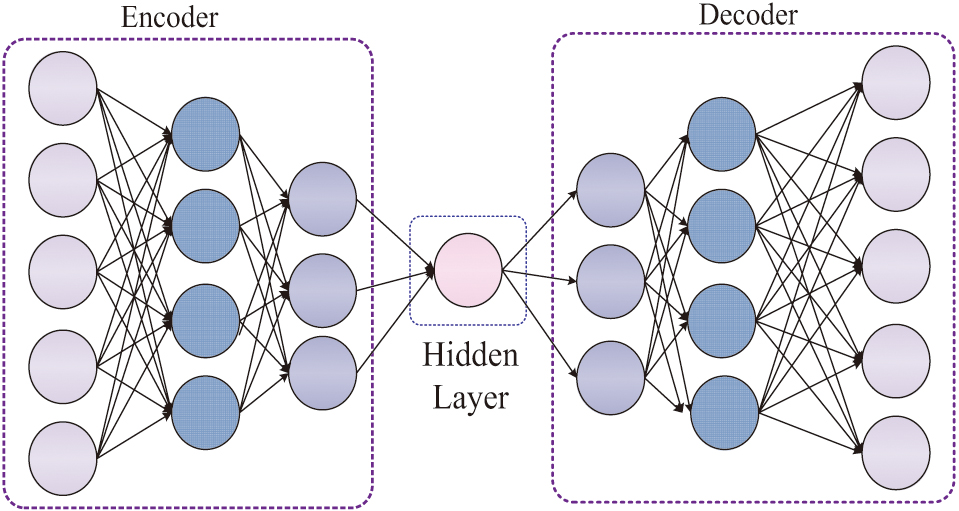
Based on the input data, the random variables represent the VAE as an unsupervised generative learning [28]. The input data map is compressed, unlike in conventional autoencoders. A useful property in SDP is one that improves defect detection and captures intricate relationships. The VAE key components are the encoder and decoder.

The below expression formulates the VAE generative model:

q (y, z) = q (y | a) q (a)

(9)

From this, the latent representation and observed data are described as $a$ and $y$ , respectively. Over $a$ , the prior distributions are assumed using a generative process, and the Gaussian distribution is selected:

q (a) = M (a | o, J)

(10)

Smooth interpolation among data points is facilitated, generalization is improved, and structured distributions are followed. However, the true posterior $q (a | y)$ , which represents the actual distribution of latent variables given input data, is generally intractable due to its complex nature. To address this, VAE approximates the posterior using a variational distribution modeled as another Gaussian:

r (a | y) = M (a | μ (y), σ (y))

(11)

where the mean

μ (y)

and variance

σ (y)

are functions of

y

, learned through a neural network. These parameters determine how the latent representation is distributed, allowing the model to capture variability in software features, such as complexity, coupling, and code churn. The training of VAE is based on maximizing the log-likelihood of the input data, but since directly computing

\log q (y)

is complex, it is rewritten using the evidence lower bound (ELBO):

\log q (y) = L M (r (a | y) | | q (a | y)) + M

(12)

where

L M

denotes the divergence term, which qualifies the difference among the approximate posteriors, ensuring that the learned latent space aligns with the prior distribution. Since divergence is

L M

always non-negative, exploiting

\log q (y)

is equivalent to exploiting

M

, which served as an optimization objective for VAE. The ELBO expression is given by:

M = F_{r (a | y)} \log q (y | a) - L M (r (a | y) | | q (a))

(13)

The first term represents the reconstruction loss, which ensures that the generated output is similar to the original input. In SDP, this corresponds to accurately reconstructing software metrics, preserving relevant defect patterns. The additional term reduces the $L M$ divergence between the approximate posterior and the prior, ensuring that latent representations remain smooth and well structured. The $L M$ divergence between two distributions $r (y)$ and $q (y)$ is mathematically defined as:

L M (r (y) | | q (y)) = \sum_{y} r (y) \frac{r (y)}{q (y)} = F_{r (y)} \frac{r (y)}{q (y)}

(14)

In unseen software modules, defects are predicted, and model generalization is allowed, reducing overfitting. Where $a$ learns the latent model and defect classification use an informative feature space. Predictive performance is enhanced, and the representations train the classifier. According to software systems, subtle defect-inducing patterns are enabled to leverage VAE. The optimization model subjected $S_{p}$ as the software defect predicted. The architecture of VAE can be shown in Fig. 2.

i)CBOAThe COA [29] is a nature-inspired metaheuristic approach that mimics the movement and social foraging behavior of crayfish. It uses swarm intelligence, in which individual crayfish interact and communicate to collectively find optimal solutions. This technique has been widely applied in solving optimization problems, particularly in training machine learning models, as it enhances parameter selection and improves predictive accuracy. By efficiently exploring the search space, COA helps refine model generalization and convergence speed, making it particularly effective for complex tasks such as fault detection and anomaly identification. However, a significant limitation of COA is its tendency to get trapped in local optima, leading to premature convergence and suboptimal solutions. This occurs because COA, like many swarm-based algorithms, may prioritize exploitation over exploration, limiting its ability to fully traverse highly complex search spaces. As a result, the algorithm sometimes fails to escape local minima, affecting overall model performance. To overcome this limitation, the BOA [30] is introduced as a complementary approach. An intelligent hunting mechanism inspires BOA. The search diversity is enhanced, and escape from local optima is enabled by incorporating BOA. The BOA ensured adaptability and better search space, preventing stagnation during the optimization process. By incorporating BOA into machine learning model training, we can significantly enhance the optimization process, leading to better convergence, improved parameter tuning, and higher predictive accuracy.

Fig. 2. Architecture of VAE.

1).INITIALIZATION

The initialization of the solution is represented in (15):

Z = [Z_{1}, Z_{2, \dots,} Z_{P}] = [\begin{matrix} Z_{1, 1} & \dots & Z_{1, l} & \dots & Z_{1, \dim} \\ ⋮ & \dots & ⋮ & \dots & ⋮ \\ Z_{k, 1} & \dots & Z_{k, l} & \dots & Z_{k, \dim} \\ ⋮ & \dots & ⋮ & \dots & ⋮ \\ Z_{P, 1} & \dots & Z_{P, l} & \dots & Z_{P, \dim} \end{matrix}]

(15)

where

Z

denotes the position of the population,

P

symbolizes the quantity of populations,

\dim

refers to the dimension of the population, and

Z_{k, l}

represents the position of the individual

k

in the

l

dimension.

2).FINDING ERROR

The optimal solution is calculated with error and can be represented in (16):

{Mean Squared Error (MSE)}_{error} = \frac{1}{n} \sum_{h = 1}^{n} [C_{b} - S_{p}]

(16)

where

C_{b}

denotes the expected outcome and

S_{p}

refers to the predicted software defect data from the VAE.

3).EXPLORATION PHASE

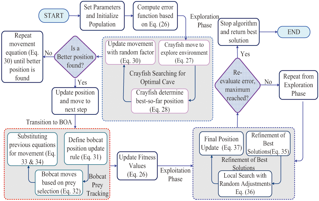
During the exploration phase, the crayfish initially explore their environment to locate the optimal cave, which serves as a promising solution. The movement is governed by:

Y_{shade} = (Y_{H} + Y_{M}) / 2

(17)

where

Y_{H}

denotes the optimal position so far attained by the number of iterations and

Y_{M}

represents the current population optimal solution:

Y_{j, k}^{u + 1} = Y_{j k}^{u} + D_{2} \times r a n d \times (Y_{shade} - Y_{j, k}^{u})

(18)

D_{2} = 2 - (\frac{u}{U})

(19)

where

u

denotes the current iteration number,

u + 1

denotes the iteration number on the next generation,

D_{2}

denotes the decreasing curve, and

U

denotes the maximum iteration. Substituting

D_{2}

in (20),

Y_{j, k}^{u + 1} = Y_{j k}^{u} + 2 - (\frac{u}{U}) \times r a n d \times (Y_{shade} - Y_{j, k}^{u})

(20)

where

Y_{j, k}^{u + 1}

and

Y_{j k}^{u}

describe the updated position of the current iteration and position. This exploration phase naturally transitions into the BOA by incorporating the concept of prey tracking. Here, the optimal cave locations identified by the crayfish are treated as prey, and bobcats simulate a tracking behavior to further refine the search. Assume,

x_{m, n}^{y} = Y_{j k}^{u}

x_{m, n}^{y + 1} = Y_{j, k}^{u + 1}

and

x_{m, n}^{best} = Y_{j, k}^{best} x_{m, n}^{y + 1} = x_{m, n}^{y} + (1 - 2 r_{m n}) \cdot (S P_{m, n} - I_{m . n} \cdot x_{m, n}^{b e s t})

(21)

x_{m, n}^{y} = x_{m, n}^{y + 1} - (1 - 2 r_{m n}) \cdot (S P_{m, n} - I_{m . n} \cdot x_{m, n}^{best})

(22)

where

x_{m, n}^{y + 1}

denotes the updated bobcat position in the next iteration,

x_{m, n}^{y}

denotes the current bobcat position,

S P_{m, n}

denotes the selected prey’s position,

I_{m, n}

denotes the influence factor, and

x_{m, n}^{best}

denotes the best bobcat position. Assume that

r_{m, n} = r_{j, k}, S P_{m, n} = S P_{j, k}, I_{m, n} = I_{j, k} .

Substitute the assumption in equation (23):

Y_{j, k}^{u} = Y_{j, k}^{u + 1} - (1 - 2 s_{j, k} - J_{j, k} \cdot Y_{j, k}^{best})

(23)

Apply equation (23) in (20)

Y_{j, k}^{u + 1} = Y_{j, k}^{u + 1} - ((1 - 2 s_{j, k}) \cdot (S P_{j, k} - J_{j, k} \cdot Y_{j, k}^{b e s t})) + (2 - \frac{u}{U}) \times r a n d \times (Y_{s h a d e} - Y_{j, k}^{u})

(24)

The best achieved position and adjustment factors are represented as $Y_{j, k}^{best}$ and $J_{j, k}$ , respectively. The search process is more effective through the integration of bobcat’s prey hunting with preliminary cave explorations of crayfish. The promising solutions with exploration and search are refined.

The global optimization capabilities are enhanced, and premature convergence is minimized, thereby balancing exploitation and exploration.

4).EXPLOITATION PHASE

From broad exploration to fine-tuning solutions, the shifts focus on the exploitation phase, ensuring rapid convergence. The updated position is demonstrated as follows:

Y_{j, k}^{u + 1} = Y_{j, k}^{u + 1} - Y_{a, k}^{u} + Y_{shade}

(25)

a = r o u n d (r a n d \times (O - 1)) + 1

(26)

Y_{j, k}^{u + 1} = (Y_{j, k}^{u} - Y) \times q + q \times r a n d \times Y_{j, k}^{u}

(27)

The random binary adjustment factor and scaling coefficients are represented as $a$ and $q$ . To achieve more accuracy, crucial model parameter fine-tuning plays a better role in optimizing the VAE. For effective and accurate fault detection, the training process is optimized, and the prediction tasks are handled. The model performance of CBOA is significantly improved, and overall performance is enhanced.

5).RE-EVALUATE THE ERROR

The error is recalculated, in which it has a lower error with the solution. Figure 3 shows the CBOA flowcharts.

Fig. 3. Flowchart for CBOA.

E.OPTIMIZE THE TERMINATION CONDITION

The collective movement of fish and birds is the metaheuristic algorithm called PSO [31]. According to the search space, the position and velocity are updated as candidate solutions. The parameters are effectively fine-tuned. The termination condition is adjusted, and optimal parameter values are determined. The undersampling process is normalized, and the termination condition is optimized by using this hybrid strategy. The premature convergence is avoided, and the search capability is improved by PSO combining with CBOA. The PSO integrates CBOA to enhance optimization. CBOA introduces diverse movement strategies inspired by crayfish and bobcats, improving search diversity and avoiding premature convergence. As the CBOA update in Equation (24) guides the search process, its influence is integrated into the PSO framework. The PSO update equations are then refined as follows:

y_{j}^{u + 1} = y_{j}^{u} + w_{j}^{u + 1}

(28)

W_{j}^{u + 1} = x w_{j}^{u} + d_{1} s + (Q_{best}^{u} - y_{j}^{u}) + d_{2} s_{2} (h_{best}^{u} - y_{1}^{u})

(29)

Y_{j}^{u + 1} = y_{j}^{u} + [x w_{j}^{u} + d_{1} s + (Q_{best}^{u} - y_{j}^{u}) + d_{2} s_{2} (h_{best}^{u} - y_{1}^{u})]

(30)

Assume

y_{j}^{u + 1} = Y_{j, k}^{u + 1}, y_{j}^{u} = Y_{j, k}^{u}, w_{j}^{u} = W_{j, k}^{u}

Substitute the assumption in equation (30),

Y_{j, k}^{u + 1} = Y_{j, k}^{u} + [x w_{j, k}^{u} + d_{1} s + (Q_{bes t_{j, k}}^{u} - Y_{j, k}^{u}) + d_{2} s_{2} (h_{best}^{u} - Y_{j, k}^{u})]

(31)

Y_{j, k}^{u + 1} = Y_{j, k}^{u} + [x w_{j, k}^{u} + d_{1} s Q_{bes t_{j, k}}^{u} - d_{1} s Y_{j, k}^{u} + d_{2} s_{2} h_{best}^{u} - d_{2} s_{2} Y_{j, k}^{u}]

(32)

Y_{j, k}^{u + 1} = Y_{j, k}^{u} [1 - D_{1} s_{1} - D_{2} s_{2}] + (x w_{j, k}^{u} + Q_{bes t_{j, k}}^{u} + d_{2} s_{2} h_{best}^{u})

(33)

Y_{j, k}^{u} [1 - D_{1} s_{1} - D_{2} s_{2}] = Y_{j, k}^{u + 1} - ((x w_{j, k}^{u} + Q_{bes t_{j, k}}^{u} + d_{2} s_{2} h_{best}^{u}))

(34)

Y_{j, k}^{u} = \frac{1}{1 - D_{1} s_{1} - D_{2} s_{2}} [Y_{j, k}^{u + 1} - (x w_{j, k}^{u} + Q_{bes t_{j, k}}^{u} + d_{2} s_{2} h_{best}^{u})]

(35)

Y_{j, k}^{u + 1} = [Y_{j, k}^{u + 1} - ((1 - 2 s_{j, k}) \cdot (S P_{j, k} - J_{j, k} \cdot Y_{j, k}^{best})) + (2 - \frac{u}{U})] \times r a n d \times (Y_{shade} - [\frac{1}{1 - D_{1} s_{1} - D_{2} s_{2}} (Y_{j, k}^{u + 1} - (x w_{j, k}^{u} + Q_{bes t_{j, k}}^{u} + d_{2} s_{2} h_{best}^{u}))])

(36)

Substitute equation (35) in (25),

Y_{j, k}^{u + 1} - Y_{j, k}^{u + 1} + \frac{Y_{j, k}^{u + 1}}{1 - D_{1} s_{1} - D_{2} s_{2}} = [- ((1 - 2 s_{j, k}) \cdot (S P_{j, k} - J_{j, k} \cdot Y_{j, k}^{best})) + (2 - \frac{u}{U})] \times r a n d \times (Y_{shade} + [\frac{1}{1 - D_{1} s_{1} - D_{2} s_{2}} (x w_{j, k}^{u} + Q_{bes t_{j, k}}^{u} + d_{2} s_{2} h_{best}^{u})])

(37)

Y_{j, k}^{u + 1} = (1 - D_{1} s_{1} - D_{2} s_{2}) + [\begin{matrix} (- ((1 - 2 s_{j, k}) \cdot (S P_{j, k} - J_{j, k} \cdot Y_{j, k}^{best})) + (2 - \frac{u}{U})) \cdot r a n d \cdot \\ (Y_{shade} + [\frac{1}{1 - D_{1} s_{1} - D_{2} s_{2}} (x w_{j, k}^{u} + Q_{bes t_{j, k}}^{u} + d_{2} s_{2} h_{best}^{u})]) \end{matrix}]

(38)

The combination of PSO and CBOA provides a refined, adaptive approach to optimizing termination conditions, thereby enhancing the selection of the defective-to-non-defective module ratio and iteration limits. The termination condition is crucial in undersampling, as it determines when to stop reducing the majority class while preserving sufficient training data. By dynamically optimizing parameters such as the undersampling ratio and the maximum number of iterations, PSO and CBOA effectively prevent overfitting and underfitting, ensuring better model generalization. Fine-tuning the termination point achieves an optimal balance between defective and non-defective modules, ultimately improving defect detection accuracy. This prediction, which comprises both defective and non-defective modules, ensures a well-balanced dataset, thereby enhancing predictive performance. The defective can be denoted as $d_{f}$ , and the non-defective can be denoted as $d_{n o}$ . The term $d_{f}$ is subject to the SGRAN for the classification.

F.SGRAN FOR CLASSIFICATION

The SGRAN integrates graph-based consistency correction and attention-driven feature enhancement for robust classification. It comprises two key modules: the graph relearn network (GRN) [32] and the scalable attention network (SAN) [33]. GRN stabilizes classification via graph-structured relearning, while SAN refines representations with hierarchical attention. This combined architecture ensures consistent, context-aware classification outcomes. Figure 4 shows the architecture of SGRAN.

i)GRNGRN is a two-phase graph-based learning framework that enhances classification performance by identifying and correcting unstable classification via a relearning process. The GRN enhances software defect classification by identifying and correcting unstable classification over training epochs. It helps to stabilize outcomes and improve reliability by refining instance classification that fluctuates across graphs using graph structure and neighbor consistency. GRN can be chosen for its robust mechanism for detecting classification inconsistencies and its ability to adaptively correct them using neighborhood-based learning. In the pre-predict phase, GRN uses a graph dense encoder (GDE) to extract deep structural features from the input data. The representation is updated using:
$d_{f} = σ (L a p {\hat{Y}}^{m} X_{l} + Y^{u} Re s_{l} + {\hat{Y}}^{m} E_{l})$ (39)
where $d_{f}$ denotes the input from the prediction output, $Lap = E - B$ is a Laplacian matrix, ${\hat{Y}}^{m}$ denotes the output of the previous layer, $X_{l}$ , $Re s_{l}$ , and $E_{l}$ denote the learnable weight matrix, and $σ$ denotes the activation function. In matrix $Q$ , the last $F$ epochs over classification are collected. The pulse matrix $Q^{'}$ is generated for tracking classification consistency:
$q_{j, k}^{'} = {\begin{matrix} 1 & i f q_{j, k} \neq q_{j, k + 1} \\ 0 & O t h e r w i s e \end{matrix}$ (40)
Based on the time, the classification variations are highlighted with binary functions. The temporal classification characteristics compute the similarity matrix:
$x_{j, k} = \sum_{l = 0}^{O} \exp (- \frac{{‖ Q_{j}^{'} - Q_{l}^{'} ‖}^{2}}{2 σ^{2}})$ (41)
The feature variance is $σ^{2}$ , and the below formula constructs the Laplacian matrix:
$L a p_{t} = E_{t} - X_{t}$ (42)
The matrix formed degree $X_{t}$ is denoted as $D_{t}$ . The informative sample set and the SAN output is $J_{G R N}$ .
ii)SANThe SAN obtains the output from GRN, and it performs final classification. Both channel and spatial-scale attention mechanisms are incorporated into the design of SAN. To distinguish both defective and non-defective instances, both global and local semantic information are preserved, and the features across multiple receptive fields are effectively extracted. More precise and efficient classification is achieved by leveraging channel-wise, scalable spatial mechanisms in SAN. The final reconstruction unit incorporates depth-related attention blocks (DRABs). The initial representations are generated by input $J_{G A N}$ :
$J_{P} = I_{S P U} (J_{G R N})$ (43)
The Deep Reconstruction Unit (DRU) refines the representations:
$J_{D R U} = I_{D R U} (J_{P})$ (44)
The expression below shows the classification output:
$J_{O U T} = I_{R E C O N} (J_{D R U} + J_{P})$ (45)
In parallel fashion, multiple DRABs are arranged within the deep refined units. Based on two parallel streams, the previous blocks processed each DRAB:
$J_{D R A B_{m}}^{(1)} = I_{D R A B} (J_{D R A B_{m - 1}}^{(1)})$ (46)
$J_{D R A B_{o}}^{(2)} = I_{D R A B} (J_{D R A B_{m - 1}}^{(2)})$ (47)
The outputs are concatenated and passed through a fusion layer:
$J_{D R U} = I_{fuse} (C o n c a t (J_{D R A B_{1}}^{(1)}, …, J_{D R A B_{M}}^{(1)}))$ (48)
From GRN outputs, a scalable attention mechanism is added to ensure broader contextual cues and local irregularities. Defective classes such as performance defects, syntax errors, functional defects, and functional errors are classified correctly. Table II outlines the overall proposed pseudocode.

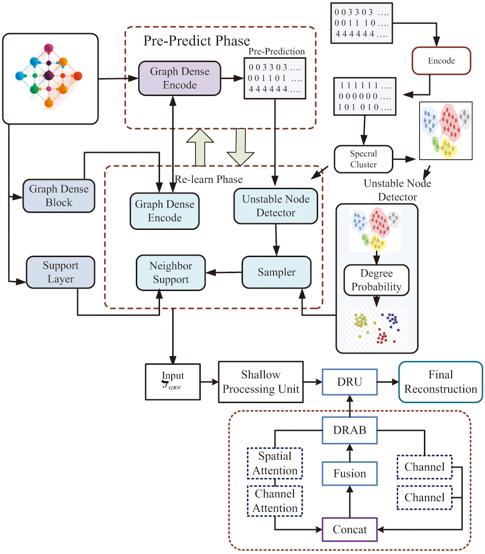Fig. 4. Architecture of SGRAN.

Table II. Overall proposed methodology pseudocode

def collect_and_preprocess():

data = collect_data()

data = impute_missing_values(data)

normalized_data = z_score_normalization(data)

return normalized_data

def train_and_optimize(data):

undersampled_data = undersample(data)

VAE_model = train_VAE(undersampled_data)

optimized_params = optimize_CBOA(VAE_model)

final_model = optimize_PSO(optimized_params)

return final_model

def predict_defects(final_model):

predictions = classify_defects(final_model)

return predictions

def refine_with_GRN(data, predictions):

graph_features = graph_dense_encoder(data, predictions)

pulse_matrix = compute_pulse_matrix(predictions)

similarity_matrix = compute_similarity_matrix(pulse_matrix)

laplacian_matrix = construct_laplacian(similarity_matrix)

refined_features = graph_refinement(graph_features, laplacian_matrix)

return refined_features

def classify_with_SAN(refined_features):

initial_representation = Self-Attention Processing Unit (SPU) (refined_features)

deep_representation = DRU(initial_representation)

final_output = reconstruct_output(deep_representation)

return final_output_class

IV.EXPERIMENTAL RESULTS

This section analyzes the experimental results. Performance metrics that provide a comparative overview of the models are used for SDP. The accuracy, precision, recall, and F1-score are used as key performance indicators, offering insight into the model’s effectiveness in detecting defects. Additionally, error metrics are analyzed to assess the predictive reliability and precision of the models. These evaluation metrics are essential for understanding the strengths and weaknesses of different classification approaches. The results provide a comprehensive comparison, highlighting the advantages of the proposed model over existing methods.

A.SYSTEM CONFIGURATIONS

The system configuration included a 2.15 GHz processor, 128 GB of RAM, Windows 10 OS, and an NVIDIA RTX 4090 (24 GB VRAM) GPU, along with Python 3.12.7 as the programming language. The VAE was trained for 20 epochs. This setup ensures robust performance and scalability during model development. The summary of the experimental setup is outlined in Table III.

Table III. Summary of experimental setup

Component	Specifications
Processor	2.15 GHz
RAM	128 GB
GPU	NVIDIA RTX 4090 (24 GB VRAM)
Operating system	Windows 10
Programming language	Python 3.12.7
Integrated Development Environment (IDE) and tools	Visual Studio Code and Jupyter Notebook
Frameworks and libraries	TensorFlow 2.12, PyTorch 2.1, Scikit-learn 1.5, Pandas, NumPy

B.DATASET EXPLORATION

Input data are collected from the AEEEM [34], ReLink [35], PROMISE [36], SOFTLAB [37], and NASA [38] datasets, which are widely used for SDP. The datasets are split into training (70%), testing (20%), and validation (10%). The AEEEM datasets consist of five open-source Java projects (Eclipse, Equinox, Lucene, Mylyn, and PDE) and include both static code and change metrics to classify instances. It contains approximately 19,945 instances, with around 13,962 used for training and 5,983 for testing. The ReLink dataset, derived from open-source repositories such as Apache, Safe, and ZXing, links bug reports to commit logs to support cross-project defect prediction (CPDP), comprising about 11,618 instances, with 8,132 for training and 3,486 for testing. The PROMISE dataset is a widely used benchmark collection of static code attributes, including Lines of Code (LOC), complexity, and coupling, gathered from multiple open-source and proprietary projects, with defect labels assigned based on historical bug reports. 3,000 test and 7,000 training samples are used across 10,000 instances. In the SOFTLAB dataset, there are 1050 test and 2450 training instances, for a total of 3500 instances. The Metrics driven prediction (MDP) complies with the NASA dataset and has 4800 test and 11200 training instances out of 16000. The predictive module valuations and developments are enabled.

Table IV shows that the SGRAN configuration consists of two main modules, GRN and SAN, each with its own hyperparameters. For the GRN module, the GDE layers range from 2 to 3, using either Graph Convolutional Network (GCN) or Graph Attention Network (GAT), with hidden dimensions of 64 or 128 and Rectified Linear Unit (ReLU) activation functions. It employs a pulse matrix window of 5–10 epochs, a similarity threshold of 0.7, and 2–5 relearn iterations, while the Laplacian smoothing factor is fixed at 0.1. In the SAN module, the SPU output dimension is either 64 or 128, and the DRU depth varies from 3 to 5 layers. The DRAB uses hidden dimensions of 64 or 128, with spatial attention kernel sizes of 3 × 3 or 5 × 5. The channel attention ratio is set at 1/8 or 1/16, and the attention fusion method is Concatenate followed by a Convolution layer. Lastly, the reconstruction unit consists of 1–2 fully connected layers.

Table IV. Settings for SGRAN configuration

Module	Hyperparameter	Value/range
GRN	GDE layers	2–3
	Hidden dimension	64 or 128
	Activation function	ReLU
	Pulse matrix window (epochs)	5–10
	Similarity threshold	0.7
	Relearn iterations	2–5
	Laplacian smoothing factor	0.1
SAN	SPU output dimension	64 or 128
	DRU depth	3-5
	DRAB hidden dimension	64 or 128
	Spatial attention kernel size	3 × 3 or 5 × 5
	Channel attention ratio	1/8 or 1/16
	Attention fusion method	Concatenate + Conv
	Reconstruction unit	1–2 Fully connected layers

C.VISUALIZATION FOR UNDERSAMPLING

Figure 5 shows the principal component analysis (PCA) visualization of the distribution of predictions before and after applying undersampling across five datasets: AEEM, Relink, PROMISE, SOFTLAB, and NASA. Each dataset’s data points are color-coded to represent four categories like non-defect and defect predictions both before and after undersampling. PCA reduces the feature space to two principal components, making it easier to visualize changes in the distribution. The horizontal axis represents PCA Component 1, while the vertical axis shows PCA Component 2. After undersampling, a more balanced and tighter clustering of defect and non-defect predictions can be observed. This visualization highlights how undersampling affects the spread and structure of the data used for prediction.

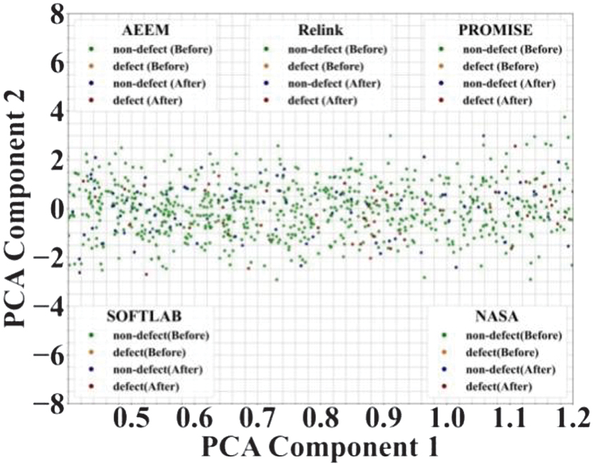Fig. 5. PCA visualization of prediction distributions before and after undersampling for five datasets.

D.ANALYSIS OF TRAINING AND TESTING

Figure 6 presents a comprehensive analysis of testing and training performance across 100 epochs for five datasets, AEEM, Relink, PROMISE, SOFTLAB, and NASA.

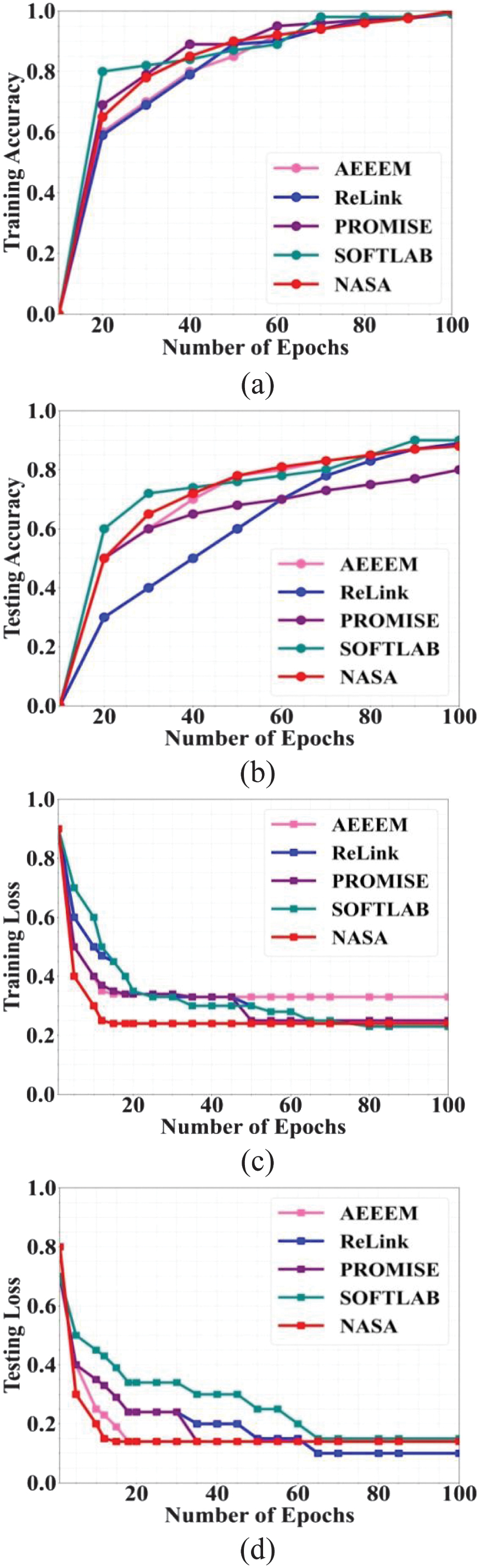Fig. 6. Training and testing performance across epochs for five datasets: (a) training accuracy, (b) testing accuracy, (c) training loss, and (d) testing loss.

The training accuracy, as shown in Fig. 6 (a), indicates stronger model training and ranges from 0.95 to 0.99. In Fig. 6 (b), the lower generalization performance is slightly improved, and the accuracy fluctuates between 0.75 and 0.9. The training loss trend is shown in Fig. 6 (c). During training, the effective error is minimized and steadily stabilizes at 0.25 and 0.35. The low error prediction is confirmed, and the test loss ranges from 0.12 to 0.19 in Fig. 6 (d). According to the middle behavior, consistency is highlighted in the performance curve. Across diverse datasets, robust performance with more reliable training convergence is demonstrated.

E.EVALUATING PERFORMANCES USING STATISTICAL PARAMETERS

For defect prediction, various models used for comparative results are described in Fig. 7. The recall is 72.05%, the F-score is 75.35%, the precision is 84.35%, and the accuracy is 82.32% for CNN-SVM [17]. For Convolutional Neural Network (CNN) [24], recall is 79.25%, F-score is 79.45%, precision is 70.12%, and accuracy is 89.25%. For Enhanced Harris Hawks Optimization with Evolutionary Crossover (EHHO-EC) [19], the findings are 85.76% recall, F-score of 81.11%, precision of 70.12%, and accuracy of 86.05%. For the proposed VAE-CBOA, the findings are 97.99% recall, F-score are 99.01%, precision of 98.96%, and accuracy of 99.05%. The proposed work achieves minimal false positives and more effective results based on the comparison analysis.

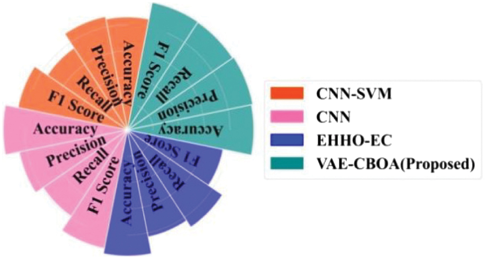Fig. 7. The SDP model analysis using various measures.

State-of-the-art studies on various classification models are described in Fig. 8. The approaches, namely K-Nearest Neighbors (KNN) [17], ANN [22], and Support Vector Machine (SVM) [19], along with the proposed SGRAN, demonstrate better performance. The recall is 70.35%, and precision is 79.12%; precision is 84.26% for ANN, and accuracy is 78.12% for KNN. However, the performance of the proposed method is 97.92% F1-score, 98.92% recall, 99.01% precision, and 98.02% accuracy. The classification performance significantly improved, and optimal results were obtained. Over the existing model, the reliability and robustness are effectively highlighted.

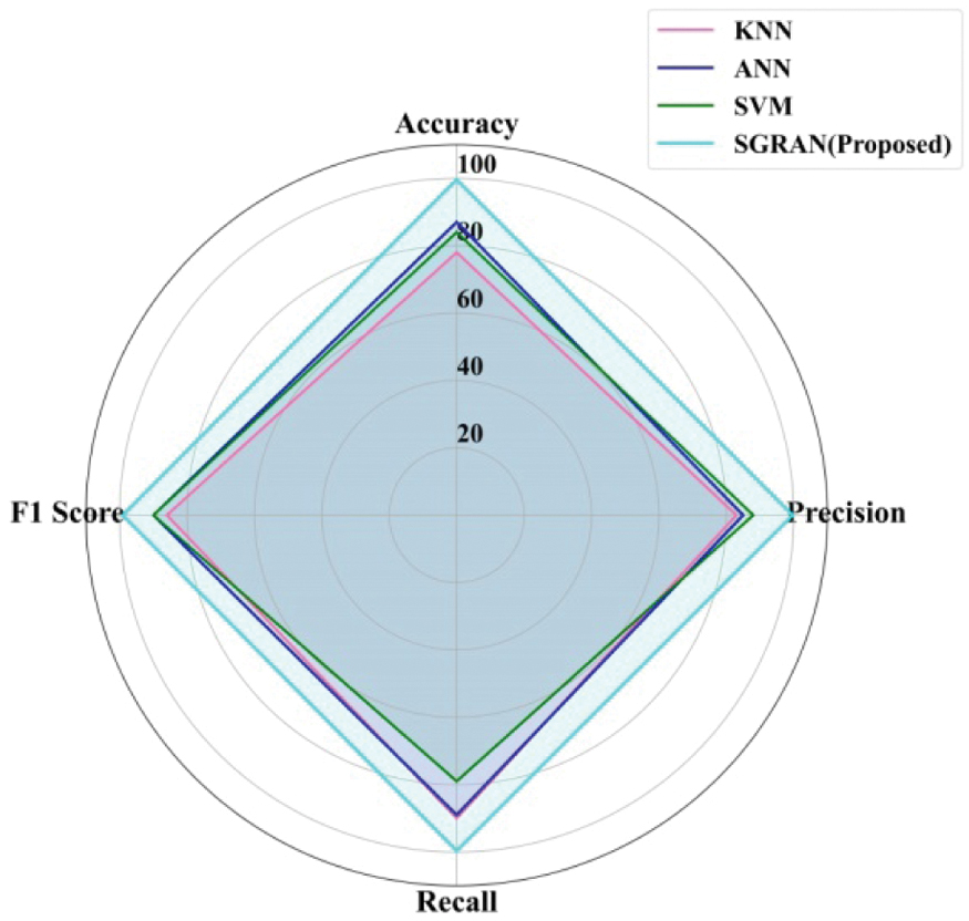Fig. 8. Classification of the proposed model with existing models.

The comparison results over various error metrics are displayed in Fig. 9. The existing method, SVM, demonstrates an MSE of 0.3, an Mean Absolute Error (MAE) of 0.58, and a MAPE of 0.8. The findings achieve 0.6 MAPE, 0.4 MAE, and 0.13 MSE for KNN; also, 0.9 MAPE, 0.48 MAE, and 0.2 MSE for ANN. The most promising results are observed, and the proposed model achieves the highest SGRAN among all the evaluated models. In the proposed work, 0.4 MAPE, 0.3 MAE, and 0.09 MSE metrics are achieved. More reliable and precise classification is provided, resulting in better results.

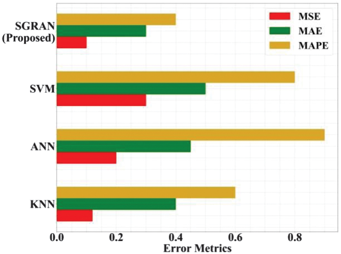Fig. 9. Error metrics evaluation for classification models.

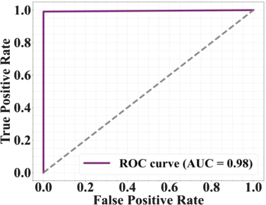
Figure 10 displays the proposed ROC performances. The model’s performance across threshold levels is plotted. The proposed classification model, SGRAN, has the AUC of 0.98. The substantial deviation from the diagonal dashed line indicates random classification.

Fig. 10. ROC performances.

F.FITNESS FUNCTION

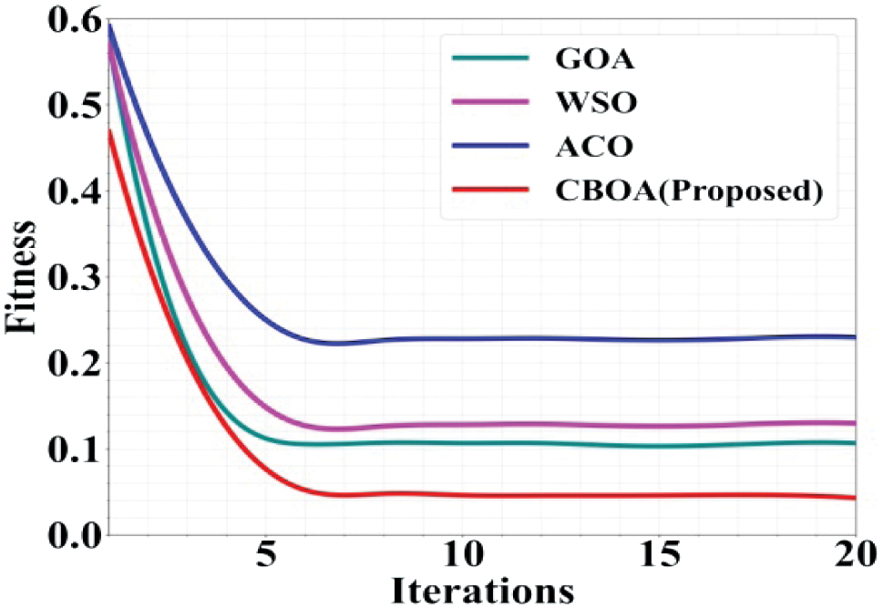
Figure 11 shows the convergence performance analysis of the proposed hybrid optimization over the 20 iterations. The existing optimization methods, like GOA [22], have the fitness of 0.13, WSO [19] has the accuracy of 0.15, and Ant Colony Optimization (ACO) [24] has the accuracy of 0.28. The proposed hybrid optimization, CBOA, outperforms the existing methods by achieving a fitness value of 0.05. Thus, the proposed model has the lowest error rate, which means training the prediction parameter should be more accurate.

Fig. 11. Convergence performance analysis.

G.ABLATION STUDY

The ablation study is displayed in Table V, which compares the performance of three models, namely DQN, feedforward neural network (FNN), and the proposed SGAN, using four evaluation metrics. DQN archives an accuracy of 83% and a precision of 79%. FNN achieves an accuracy of 64.44%, a precision of 69.29%, and a recall of 66.75%. The SGAN achieved the best results, with 98.02% accuracy, 99.01% precision, 98.92% recall, and an F1-score of 97.92%.

Table V. Ablation study

Models	Accuracy (%)	Precision (%)	Recall (%)	F1-scoce (%)
DQN	83	79	62	78
FNN [18]	64.44	69.29	66.75	63.80
SGAN (proposed)	98.02	99.01	98.92	97.92

V.DISCUSSION

This work presented a new model to address the significant challenges. For undersampling, the LTRUS is employed without warping feature distributions, and the class imbalance is handled. The generalization is enhanced, and complex latent defect patterns are extracted by incorporating a VAE. Strong model tuning is guaranteed, prediction reliability is enhanced, and premature convergence is prevented by integrating the hybrid CBOA-PSO model. PSO and CBOA optimize the termination condition to balance the non-defective and defective samples. Context-aware and precise predictions are produced via SGRAN.

Based on the all-encompassing approach, the software systems are changed, and model adaptability and predictive accuracy are evaluated. To tackle data imbalance and overfitting, the software quality assurance is ensured. All things considered, this work offers an intelligent, scalable solution for next-generation defect-detection systems. To support ongoing quality assurance, the proposed model is integrated into continuous deployment or continuous integration. Potential defects are detected during build or deployment, and the newly committed source code is automatically analyzed. The faulty component is prevented from entering production. To leverage graph-based dependency analysis, the defects-prone areas are dynamically identified, and latent representations from incoming code metrics are rapidly extracted using a VAE component. Operational efficiency and software reliability are enhanced through faster release cycles, reduced debugging costs, and proactive defect detection, achieved by embedding the proposed model into development teams and the software delivery workflow. In real-world development ecosystems, the proposed model demonstrated practical relevance and deployment.

VI.CONCLUSION

This study proposed an efficient SDP model that integrates a VAE with a hybrid CBOA. The preprocessing steps including missing value imputation and Z-score normalization ensured data consistency and improved feature comparability. The LTRUS-based undersampling techniques effectively addressed class imbalance, enhancing model performance. For defect classification, the robust latent representation provided by the VAE captured intricate defect patterns and software metrics. The model training was optimized, premature convergence was prevented, and the proposed model effectively balanced both the global exploration and local search abilities of both BOA and COA. A balanced defective and non-defective module ratio was ensured, and the termination condition was fine-tuned during PSO. The generalization ability, convergence speed, and defect detection accuracy were improved. Software quality predictions were optimized, and imbalanced datasets were handled with effective findings of experimental results. Reliable defect identification was achieved with 97.99% accuracy and 98.96% precision. The F-score was 97.92%, precision was 99.01%, and the robust model was the SGRAN model. Emphasizing the enhancements was to support early defect detection. In the future, additional deep learning models and transformers will be explored and used to enhance the prediction performance defect. Practical applicability will improve the large-scale software systems. Across various software environments, diverse datasets will ensure robustness.

Hybrid Approach to Software Defect Prediction and Classification using a Variational Autoencoder and Scalable Graph Attention Network

I.INTRODUCTION

A.SOFTWARE AND ITS VULNERABILITIES

B.ROLE OF SDP AND CLASSIFICATION

C.CHALLENGES AND THE PROPOSED HYBRID APPROACH

D.MAJOR CONTRIBUTIONS

II.LITERATURE SURVEY

A.PROBLEM STATEMENT

III.PROPOSED METHODOLOGY

A.DATA COLLECTION

B.DATA PREPROCESSING

1).MISSING VALUE IMPUTATION

2).Z-Score Normalization

3).UNDERSAMPLING

D.SOFTWARE DEFECT PREDICTION

1).INITIALIZATION

2).FINDING ERROR

3).EXPLORATION PHASE

4).EXPLOITATION PHASE

5).RE-EVALUATE THE ERROR

E.OPTIMIZE THE TERMINATION CONDITION

F.SGRAN FOR CLASSIFICATION

IV.EXPERIMENTAL RESULTS

A.SYSTEM CONFIGURATIONS

B.DATASET EXPLORATION

C.VISUALIZATION FOR UNDERSAMPLING

D.ANALYSIS OF TRAINING AND TESTING

E.EVALUATING PERFORMANCES USING STATISTICAL PARAMETERS

F.FITNESS FUNCTION

G.ABLATION STUDY

V.DISCUSSION

VI.CONCLUSION

ACKNOWLEDGMENTS

COMPETING INTERESTS

FUNDING STATEMENT

COMPLIANCE WITH ETHICAL STANDARDS

REPLICATION OF RESULTS

DATA AVAILABILITY STATEMENTS

AUTHORS’ CONTRIBUTION

REFERENCES