I.INTRODUCTION
Skin cancer is among the most common malignancies, with over 1.5 million new cases and nearly 100 000 deaths annually; melanoma, though only 1% of lesions, causes over 75% of mortality [1]. Dermoscopy—a noninvasive imaging modality—reveals subsurface structures but demands specialist training and exhibits over 20% inter-observer variability [2,3]. Early computer-aided systems relied on handcrafted features (color histograms, texture descriptors, and border irregularity) with classical classifiers such as Support Vector Machine (SVMs) and random forests (RFs) [4,5].
With the advent of deep learning, CNNs have achieved dermatologist-level performance on large, curated lesion datasets such as HAM10000 and ISIC, automatically learning hierarchical features from pixels [2,6]. However, CNNs exhibit two critical limitations in high-stakes clinical settings: (i) they function as opaque “black-box” predictors with limited interpretability; and (ii) they lack robust, calibrated measures of predictive confidence, undermining trust and hindering triage decisions [7]. In high-stakes clinical settings, an overconfident yet incorrect prediction can result in serious consequences such as misdiagnosis and inappropriate treatment. This underscores the critical need for well-calibrated uncertainty estimates that help distinguish clear-cut cases from ambiguous ones. Uncertainty quantification (UQ) addresses this challenge by measuring the confidence of model predictions [6]. Broadly, uncertainty in artificial intelligence (AI) models can be categorized into two types: epistemic uncertainty, arising from gaps in the model’s knowledge due to limited training data or insufficient model capacity, and aleatoric uncertainty, reflecting intrinsic noise or ambiguity in the input data (e.g., poor image quality) [8]. Effective UQ enables AI systems to flag uncertain predictions, allowing clinicians to exercise caution or seek second opinions, thereby enhancing the reliability and safety of automated diagnostic tools. Quantifying these uncertainties allows models to express confidence: low-uncertainty predictions can be trusted directly, while high-uncertainty cases are flagged for further expert review. Numerous studies in medical imaging have shown that uncertainty estimation techniques [9]. Monte Carlo dropout (MCD) remains a practical Bayesian approximation for estimating epistemic uncertainty by retaining dropout layers at test time [10]. Concurrently, graph neural networks (GNNs) and their transformer extensions encode inter-sample relationships by treating each image as a node and defining edges via feature- or metadata-based similarity [11]. Recent work on attentive GNNs has highlighted the importance of neighbor-scoring mechanisms: Fang et al. proposed Kolmogorov–Arnold Attention (KAA) to improve how GNNs weight neighbor contributions, yielding over 20% performance gains across benchmark graphs [12]. Despite these advances, no prior skin lesion classification framework unifies graph-based relational learning with rigorous Bayesian or conformal uncertainty in a single pipeline. In neurology, population graph constructions have enhanced disease prediction [11,13,14], and in vision, conformal calibration has improved trustworthiness [15]. Yet, bridging these strengths in dermatologic imaging remains an open challenge.
To bridge this gap, we propose GraphSkinUQ, the first end-to-end framework that unifies an augmented Keras CNN and ResNet50 embeddings for feature extraction, a tunable -nearest-neighbor (k-NN) graph, a three-layer graph transformer with multi-head attention and residual connections, and MCD inference (50 stochastic passes) to compute per-node predictive entropy and calibration metrics. We validate GraphSkinUQ using accuracy, F1-score, Brier score, calibration curves, and ROC/Precision–Recall (PR) analyses, demonstrating its potential for trustworthy AI in dermoscopic diagnosis.
The remainder of this paper is organized as follows. Section II reviews related work; Section III details our architecture; Section IV presents experimental results; and Section V concludes with future directions.
II.RELATED WORKS
Research on automated skin cancer classification has progressed rapidly, motivated by the critical demand for accurate and interpretable diagnostic systems. Early studies predominantly leveraged CNNs to learn hierarchical features from dermoscopic images.
Although CNN-based models have achieved dermatologist-level performance on public benchmarks such as HAM10000 and ISIC, they present notable limitations: (i) they provide deterministic outputs without calibrated uncertainty measures, and (ii) their generalization degrades under domain shifts or data scarcity [4,5,16,17]. These challenges have catalyzed interest in integrating uncertainty estimation within deep learning pipelines.
A.CNN WITH BAYESIAN DROPOUT
Afshar et al. utilized MCD at inference to approximate predictive distributions, reporting an average accuracy of 85.65% across MNIST, HAM10000, and synthetic lesion datasets while demonstrating enhanced detection of uncertain predictions [18]. Rajeev Kumar et al. advanced this line by combining MCD with test-time augmentation (TTA) in the SkiNet framework, achieving classification accuracy of 73.65% alongside lesion segmentation and saliency-based explainability (Grad-CAM, XRAI). However, the additional segmentation and multiple inference passes introduced substantial computational overhead [19].
B.COMPACT CONVOLUTIONAL TRANSFORMERS (SKINNET-14)
Lateef et al. introduced SkinNet-14, a compact convolutional transformer (CCT) optimized for low-resolution (32 × 32) dermoscopy images. By reducing model depth and parameter count, SkinNet-14 trains in seconds per epoch yet attains up to 98.14% accuracy on HAM10000, ISIC, and PAD datasets. Its data-efficient design and aggressive augmentation addressed class imbalance, making it suitable for resource-constrained settings. Limitations include potential loss of fine-grained lesion details at ultra-low resolution and the need for real-world clinical validation to confirm generalizability [5].
C.ENHANCED CNN ARCHITECTURES (FCDS-CNN)
Patel et al. proposed the Fully Connected Deep Supervised-CNN (FCDS-CNN), which leverages extensive data augmentation, class-weighted loss functions, and transfer learning from ImageNet-pretrained backbones to tackle intra-class variability and dataset imbalance. Achieving 96% average accuracy on benchmark sets, FCDS-CNN demonstrated robust, real-time inferencing capability. Its strengths lie in computational efficiency and adaptability; however, dependency on dataset quality and limited external validation remained concerns for broader clinical deployment [16].
Ray et al. (2024) presented a comprehensive review of 107 studies on skin cancer classification covering the past 18 years, emphasizing the evolution of AI-driven dermatologic analysis. The paper traced progress from early handcrafted feature-based models to advanced deep learning frameworks such as CNNs, Generative Adversarial Network (GANs), and Vision Transformers. It also reviewed widely used datasets (HAM10000, ISIC), compared hybrid and multimodal approaches, and discusses performance evaluation metrics and optimization strategies. Importantly, the authors identified persistent challenges—including data scarcity, interpretability, and lack of standardization—and proposed future directions aimed at improving clinical integration and diagnostic reliability [20].
D.SEGMENTATION-LEVEL UNCERTAINTY
Elfatimi et al. embedded MCD and Bayes-by-Backpropagation within U-Net architectures to generate pixel-wise uncertainty maps, reporting Dice scores of 0.8809 (from-scratch) and 0.8313 (transfer learning) on ISIC-2019. While this approach enhanced lesion boundary reliability, its high computational cost and reliance on precise ground-truth annotations limited real-time applicability and scalability [21].
E.THREE-WAY DECISION BAYESIAN ENSEMBLES
Abdar et al. designed a Three-Way Decision Bayesian Deep Learning (TWDBDL) framework that unites MCD, ensemble MCD, and deep ensembles to capture diverse uncertainty modalities. This ensemble yielded 88.95% accuracy with improved calibration, but at the expense of substantially increased inference time and implementation complexity, posing challenges for deployment in time-sensitive clinical workflows [22].
F.TRANSFORMER-BASED MODELS
Guang et al. adapted Vision Transformers (ViTs) for skin lesion classification, incorporating class rebalancing and patch decomposition to reach 94.1% accuracy on HAM10000. Standard ViTs, however, lack intrinsic UQ, limiting their transparency in high-stakes medical settings [23]. Graph transformer variants—marrying self-attention with sample-relationship embeddings—remain largely unexplored in tandem with Bayesian inference. In addition to this, Adebiyi et al. conducted a comprehensive systematic review analyzing 57 studies from 2017 to 2023 that applied transformer-based models to skin lesion classification tasks. Their findings highlighted the adaptability of transformers across various skin lesion datasets, including dermoscopic, clinical, and histopathological images. The review emphasizes the utilization of pretrained models and the integration of mechanisms such as attention modules to enhance feature extraction. This work provides valuable insights into the current state of transformer applications in dermatological diagnostics and identifies potential areas for future research [24]. More recently, Zoravar et al. proposed a conformal ensemble of Vision Transformers (CE-ViTs) that explicitly addresses domain shifts in skin lesion datasets by combining an ensemble of ViTs with conformal prediction techniques. The method achieved ∼90.38% coverage of true labels, improving significantly over single model baselines. While promising in terms of uncertainty and domain adaptation, the approach still bears the computational overhead typical of ensemble-based methods [25].
G.UNCERTAINTY IN MEDICAL IMAGING
Leibig et al. explored uncertainty estimation in deep neural networks applied to disease detection, specifically diabetic retinopathy, by interpreting dropout at inference time as a Bayesian approximation. They showed that dropout-based predictive distributions allow the network to flag uncertain cases, which can then be referred for human expert review. This referral mechanism both improves overall diagnostic accuracy and aligns model behavior with clinical practice, where cases deemed uncertain by the algorithm prompt secondary evaluation [26].
Zhao et al. extended the notion of uncertainty learning to breast cancer recognition in their 2023 DOCS paper. Instead of treating all training samples as equally reliable, their framework explicitly models data uncertainty—accounting for noise and ambiguity in imaging—during feature learning. By integrating a learned uncertainty weight into the loss function, their method boosts robustness against noisy or borderline examples, yielding higher detection sensitivity and more calibrated confidence scores compared to deterministic baselines [27].
H.RELATIONAL HYBRID MODELS
Putra et al. proposed Tiny Pyramid ViG, fusing capsule networks with GNNs to model part–whole hierarchies and inter-sample dependencies, achieving 95.52% accuracy on HAM10000. The complexity of graph construction and tuning, however, increases design overhead and may hinder reproducibility [28]. Alwakid et al. (2025) proposed a graph attention network (GAT) framework that integrated CNN-derived node features for skin lesion classification. Dermoscopic images were first segmented into superpixels via Simple Linear Iterative Clustering (SLIC) to construct a region-adjacency graph, with each node described using EfficientNet-B0 embeddings. A five-layer GAT then modeled the relationships between nodes, dynamically weighting local and global dependencies. The method achieved 88.35% accuracy and 98.04% area under the curve (AUC) on the DermaMNIST dataset, outperforming conventional CNNs and GNN baselines. The approach’s robustness—achieved without data augmentation or metadata—demonstrated the strength of combining graph relational reasoning with deep visual features for multi-class skin lesion diagnosis [29].
I.GAP IN THE LITERATURE
No prior work jointly (i) uses a graph transformer to learn inter-sample relations, (ii) embeds MCD into graph-based inference, and (iii) delivers a single end-to-end pipeline from CNN features through -NN graph construction to uncertainty-aware predictions.
J.OUR CONTRIBUTION: GraphSkinUQ
We introduce GraphSkinUQ, a unified pipeline that combines CNN feature learning, graph-based relational modeling, and uncertainty estimation:
- 1.Augmented CNN Backbone. Train a lightweight Keras CNN on heavily augmented dermoscopic images (rotations, flips, shifts, shear, zoom) to extract robust features.
- 2.ResNet50 Embeddings. Remove the final layer of a PyTorch ResNet50 to obtain 2048-dimensional deep representations for each image.
- 3.k-NN Graph Construction. Build a similarity graph by connecting each embedding to its closest neighbors (validated on held-out data) via Euclidean distance.
- 4.Graph Transformer. Apply three TransformerConv layers (multi-head attention, LayerNorm, and residuals) to propagate information across the -NN graph and capture higher-order relationships.
- 5.MC-Dropout Uncertainty. At inference, perform stochastic forward passes with dropout enabled to compute:
- ○Predictive entropy .
- ○Expected calibration error (ECE) to assess confidence calibration.
GraphSkinUQ achieves ≈92% accuracy on dermoscopic benchmarks, delivers well-calibrated confidence estimates (low Brier score, favorable ECE), and is fully reproducible from raw images to uncertainty-aware predictions.
III.METHODOLOGY
The proposed framework, termed GraphSkinUQ, as shown in Fig. 1, for skin spot cancer classification comprises a sequence of integrated stages. It begins with data acquisition and augmentation, progresses through deep learning-based feature extraction and classification, followed by graph construction and Graph Transformer Network (GTN) training, and concludes with UQ through MCD. GraphSkinUQ combines three key capabilities—robust feature extraction to capture diverse lesion patterns, relational graph modeling to leverage similarities across cases, and principled uncertainty estimation to flag ambiguous predictions—ensuring both high diagnostic accuracy and trustworthy confidence measures for safer skin cancer screening.
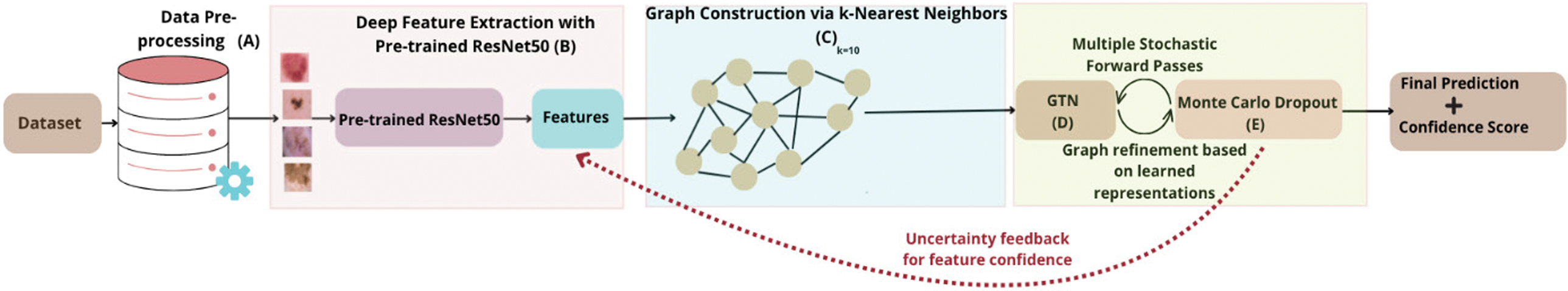 Fig. 1. Overall architecture of GraphSkinUQ, illustrating feature extraction, graph construction, transformer reasoning, and MC dropout inference.
Initially, the dataset—already organized into subdirectories for the two classes (benign and malignant)—undergoes extensive preprocessing and augmentation. Using TensorFlow’s ImageDataGenerator, each image is normalized (using a scaling factor ) and augmented via random rotations (up to 25°), horizontal flips, width and height shifts (10%), shearing, and zooming (10% each). In mathematical terms, given an input image , the normalized image is defined as:
and subsequent augmentations are applied using affine transformations. For instance, an original benign image of size 224 × 224 pixels from the Kaggle dataset is normalized by dividing pixel intensities by 255, resulting in values between 0 and 1. Random transformations such as 15° rotation and 10% zoom produce augmented versions that help the CNN learn invariance to orientation and scale.A.DETAILED ARCHITECTURE
The overall architecture of GraphSkinUQ comprises several interconnected modules, each governed by mathematically rigorous operations:
1).CNN FOR CLASSIFICATION
During CNN training with Keras, the dataset is divided only into a training set and a validation set (20% held out for validation). A separate test split is not created at this stage.
In contrast, during the PyTorch-based feature extraction and graph modeling stage, we explicitly split the full ImageFolder dataset into 80% training, 10% validation, and 10% test subsets before building the k-NN graph and training the GTN.
The CNN consists of multiple convolutional blocks. In each block, the convolution operation is defined as:
where is the input feature map from the previous layer, denotes the weights of the layer, is the bias term, and represents the activation function (Rectified Linear Unit (ReLU) in our case). Each convolutional layer is succeeded by batch normalization and max pooling to reduce spatial dimensions. After flattening the feature maps, two fully connected (dense) layers with 256 and 128 units are applied with L2 regularization and dropout regularization. Dropout helps preventing overfitting is mathematically modeled as: where is the dropout probability and represents element-wise multiplication. The final dense layer uses a sigmoid activation for binary classification, and the loss function is defined by the binary cross-entropy: with being the ground truth and the predicted probability for the sample. The training employs the Adam optimizer with a learning rate of 0.0005, and techniques such as early stopping and learning rate reduction on plateau are applied to ensure convergence.2).DEEP FEATURE EXTRACTION WITH PRETRAINED RESNET50
A pretrained ResNet50 model, with the final classification layer removed, is used to extract high-level representations. The images are resized to pixels and normalized using ImageNet statistics. If represents an input image, the deep feature vector is obtained by:
where denotes the forward pass through ResNet50 up to the penultimate layer and is the dimensionality of the extracted feature space.After preprocessing, a sample image is passed through ResNet50, producing a 2048-dimensional feature vector. For example, one malignant image yields a feature embedding where higher activations correspond to darker, irregular lesion regions. These embeddings form the basis for subsequent graph construction.
3).GRAPH CONSTRUCTION VIA k-NNS
The extracted feature vectors are used to construct a k-NN graph. Let and be feature vectors of images and , respectively; the Euclidean distance between these vectors is given by:
For each node, connections are established with its nearest neighbors, resulting in a connectivity matrix that is later converted into an edge list suitable for processing with PyTorch Geometric’s Data class. Training, validation, and test masks are defined on this graph to enable supervised learning.
Using these embeddings, the similarity graph is built. For instance, the feature vector of Image #210 (benign) is connected to its 10 most similar nodes, such as Images #134, #598, and #623, based on Euclidean distances ranging from 0.45 to 0.63. This structure ensures that visually similar lesions share information during graph learning.
4).GTN AND HYPERPARAMETER TUNING
At the core of GraphSkinUQ lies the GTN, which leverages the relational structure within the graph. At each transformer layer, multi-head attention computes new node representations. For an input node feature matrix and adjacency information given by , the transformer convolution is formulated as:
with each head computed via: where and are learnable parameters for the attention head, and is an activation function (ReLU). Skip connections and layer normalization are integrated to enhance gradient flow and model stability. The final classification is achieved using a linear layer followed by a log-softmax function:A comprehensive grid search over learning rate, hidden channel dimensions, and dropout rates is conducted. Each configuration is trained for 300 epochs using a ReduceLROnPlateau scheduler, and the model achieving the highest validation accuracy is selected for further evaluation.
5).UQ VIA MCD
In order to quantify predictive uncertainty, GraphSkinUQ enables MCD during inference. The best-performing GTN is maintained in training mode to activate dropout. For stochastic forward passes (with ), the predictive probability for each node is averaged:
and the uncertainty is assessed via entropy: where is a small constant to prevent numerical instability.Figure 2 illustrates each step of our MCD pipeline. We start by extracting CNN features, building the 10-NN graph, and training the GTN with active dropout (steps 1–4). At inference, the “MCD?” decision node triggers stochastic forward passes (steps 5–7), whose outputs are aggregated (step 8) and converted to a Shannon entropy score (step 9) to yield a robust per-case uncertainty measure. Embedding this diagram immediately after our equations lets readers directly map theory to practice.
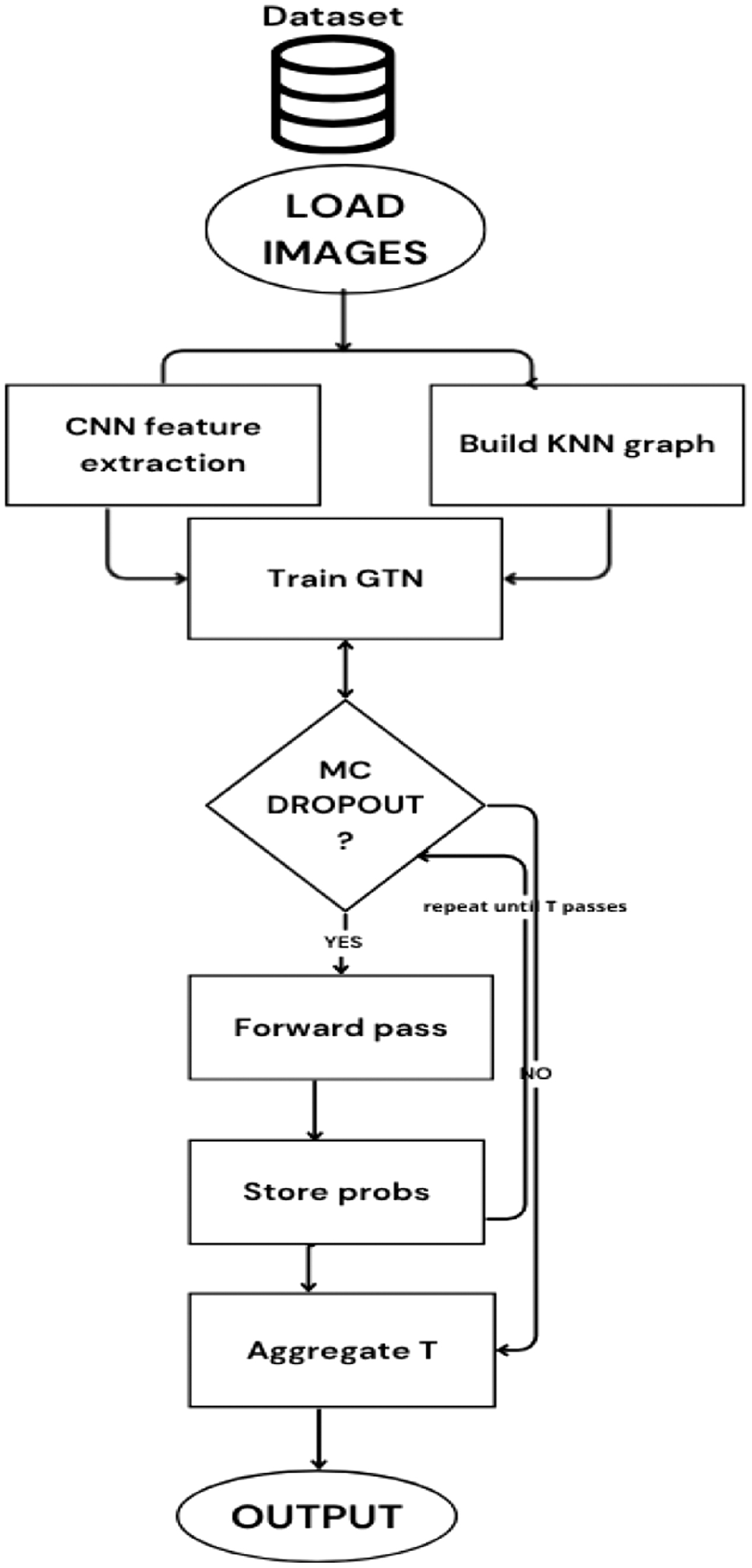 Fig. 2. Compact MC dropout uncertainty workflow for GraphSkinUQ.
B.EVALUATION METRICS
To thoroughly evaluate our approach, we employ a suite of metrics: accuracy, precision, recall, F1-score, average uncertainty, and the Brier score. Their definitions are as follows:
- 1)Accuracy measures the proportion of correct predictions out of all samples. Given true positives (), true negatives (), false positives (), and false negatives ().
- 2)Precision reflects the fraction of correctly identified positive cases among all positive predictions.
- 3)Recall (or sensitivity) represents the fraction of actual positives that are correctly recognized.
- 4)F1-Score is the harmonic mean of precision and recall, balancing the trade-off between false positives and false negatives.
- 5)Average Uncertainty is quantified via the entropy of averaged predictive probabilities obtained through MCD, for test samples and classes.
- 6)Brier Score evaluates the accuracy of probabilistic forecasts by comparing predicted probabilities with actual binary outcomes. For predictions, with the forecast probability and the true label.
IV.EXPERIMENTS AND RESULTS
In this section, we detail the experimental setup used to evaluate GraphSkinUQ. This includes a description of the dataset, experimental parameters, and the research questions addressed in our study.
A.DATASET DESCRIPTION AND STATISTICS
The dataset used in this work is obtained from Kaggle and comprises skin cancer images collected into two distinct classes: malignant and benign. In total, the dataset includes 1 497 malignant images and 1 800 benign images. Each image is preprocessed and augmented to improve generalization and address class imbalance. Table I summarizes the dataset statistics.
| Class | Number of images | Percentage |
|---|---|---|
| Malignant | 1 497 | 45% |
| Benign | 1 800 | 55% |
| Total | 3 297 | 100% |
The dataset is characterized by significant variability in image appearance due to factors such as lighting conditions, scale, and patient demographics. Extensive data augmentation is performed during preprocessing to mitigate these effects and prevent overfitting.
B.RESULTS
In this experiment, we have conducted an extensive hyperparameter tuning process for the proposed GraphSkinUQ model. Eight configurations are evaluated by varying the dropout rate, number of hidden channels, and learning rate. Table II summarizes the hyperparameter settings along with the corresponding validation and test accuracies (with test accuracy measured using MCD).
Table II. Hyperparameter tuning results for GraphSkinUQ
| Exp. | Hyperparameters | Val. acc. | Test acc. |
|---|---|---|---|
| 1 | Dropout: 0.5, hidden_chan.: 16, lr: 0.001 | 0.8602 | 0.9063 |
| 2 | Dropout: 0.5, hidden_chan.: 16, lr: 0.0005 | 0.8723 | 0.9215 |
| 3 | Dropout: 0.5, hidden_chan.: 32, lr: 0.001 | 0.8541 | 0.9124 |
| 4 | Dropout: 0.5, hidden_chan.: 32, lr: 0.0005 | 0.8541 | 0.9063 |
| 5 | Dropout: 0.3, hidden_chan.: 16, lr: 0.001 | 0.8571 | 0.9124 |
| 6 | Dropout: 0.3, hidden_chan.: 16, lr: 0.0005 | 0.8602 | 0.9003 |
| 7 | Dropout: 0.3, hidden_chan.: 32, lr: 0.001 | 0.8663 | 0.9003 |
| 8 | Dropout: 0.3, hidden_chan.: 32, lr: 0.0005 | 0.8541 | 0.9094 |
Among these configurations, Experiment 2 (with hyperparameters {dropout: 0.5, hidden_channels: 16, lr: 0.0005}) yielded the highest validation accuracy of 87.23% and a test accuracy of 92.15%.
Our hyperparameter tuning experiments indicate that a dropout rate of 0.5, 16 hidden channels, and a learning rate of 0.0005 is optimal. This configuration produced a validation accuracy of 87.23% and a test accuracy of 92.15% before MC evaluation. Following UQ, to address the role of UQ in improving model reliability and decision confidence within a high-stakes medical imaging task, we deploy our proposed model, GraphSkinUQ, a GTN equipped with MCD. This enables uncertainty estimation by sampling the predictive distribution multiple times during inference. The classification task involves binary diagnosis of skin lesions as either Benign or Malignant. Performance is evaluated using traditional metrics (accuracy, precision, recall, F1-score), alongside the average predictive entropy as a proxy for uncertainty (Table III).
C.UNCERTAINTY ANALYSIS
In this section, we present a detailed examination of the uncertainty behavior of the GraphSkinUQ model, considering both its discriminative power and calibration quality.
1).DISCRIMINATION PERFORMANCE
Figure 3 shows the ROC curve for our model, for which we report an AUC of 0.95. This high AUC indicates that GraphSkinUQ ranks true malignant cases above benign ones 95.4% of the time. Even samples whose predicted probabilities lie near the decision boundary tend to be correctly separated from clear negatives, demonstrating that the model’s confidence scores are largely meaningful.
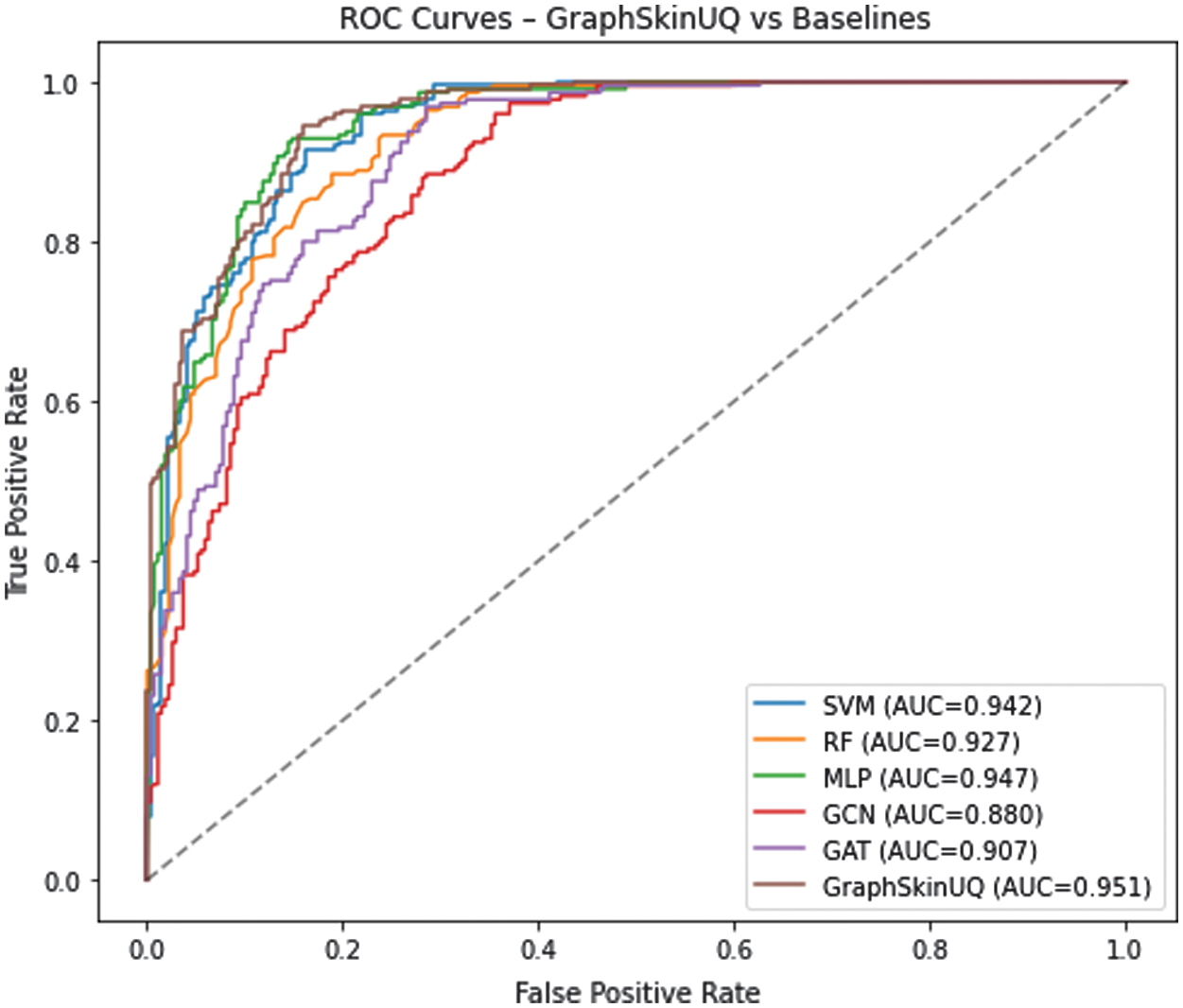 Fig. 3. ROC curve for GraphSkinUQ (AUC = 0.951).
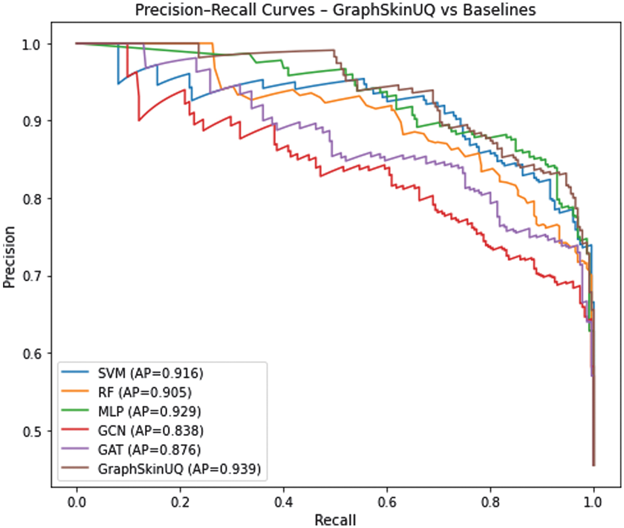
The precision–recall curve in Fig. 4 further elucidates the model’s behavior. At low recall levels (below 0.5), precision remains near 1.0, indicating that the highest-confidence positive predictions are almost always correct. As recall approaches 1.0, precision declines to approximately 0.65, marking the region where more uncertain cases contribute to false positives. The steep drop in precision between recalls of 0.75 and 1.0 defines an “uncertainty zone” in which the model’s decisions become less reliable.
2).COMPARATIVE ANALYSIS
Figures 3 and 4 present the ROC and Precision–Recall curves for all compared methods. GraphSkinUQ consistently achieves the highest AUC and AP scores, followed by multi-layer perceptron (MLP) and SVM, whereas traditional graph models (graph convolutional network (GCN) and GAT) show lower discriminative ability. These results align with the quantitative metrics in Table IX, confirming that integrating relational graph reasoning with UQ enhances both sensitivity and precision. The improvement is particularly notable in the high-recall region, indicating greater reliability for safety-critical screening tasks.
3).SOURCES OF UNCERTAINTY
While GraphSkinUQ achieves strong overall performance, we include this discussion of epistemic and aleatoric uncertainty to demonstrate how the model explicitly quantifies—and in the case of epistemic uncertainty, mitigates—areas where even high-accuracy systems naturally face ambiguity. In other words, highlighting these two uncertainty sources does not imply a fundamental weakness of GraphSkinUQ but rather underscores its built-in mechanisms for managing them:
- •Epistemic (Model) Uncertainty: Even with MCD at inference, some lesion patterns near the decision boundary remain inherently harder to learn. By sampling multiple dropout realizations, GraphSkinUQ not only measures its own confidence but also reduces overconfident errors in this “uncertain zone.” This capability is a deliberate strength, ensuring the model signals when its knowledge is limited rather than silently misclassifying.
- •Aleatoric (Data) Uncertainty: Variability in image quality or missing metadata can never be fully eliminated by training alone. GraphSkinUQ acknowledges this by reporting higher uncertainty for these cases. Far from indicating failure, this feature empowers clinicians to flag ambiguous examples for further review, turning data noise into a useful triage signal.
In sum, discussing these uncertainty types showcases GraphSkinUQ’s proactive approach: it does not simply deliver point predictions but also provides calibrated confidence estimates that improve safety and trust in real-world clinical use.
4).CALIBRATION ASSESSMENT
Beyond discrimination, well-calibrated probabilities are essential when confidence scores guide clinical decisions. We employ two quantitative metrics:
- •The Brier score, measuring squared deviation between predicted probabilities and outcomes, is 0.13.
- •The ECE, summarizing absolute differences between confidence and accuracy over bins, is 0.06.
These low values confirm that GraphSkinUQ’s confidence estimates align closely with observed frequencies. If further refinement were required, post hoc methods such as temperature scaling or isotonic regression could be applied without retraining the model.
5).QUANTITATIVE SUMMARY
Table IV aggregates key metrics:
Table III. Classification report for the best model (dropout: 0.5, hidden_channels: 16, lr: 0.0005)
| Class | Precision | Recall | F1-score |
|---|---|---|---|
| Benign | 0.92 | 0.93 | 0.93 |
| Malignant | 0.91 | 0.90 | 0.90 |
| Accuracy | 0.91 | ||
| Macro avg | 0.91 | 0.91 | 0.91 |
| Weighted avg | 0.92 | 0.92 | 0.92 |
Table IV. Overall uncertainty and performance metrics
| Metric | Value |
|---|---|
| Classification accuracy | 92% |
| ROC AUC | 0.954 |
| Average predictive entropy | 0.10 |
| Brier score | 0.13 |
| Expected calibration error (ECE) | 0.06 |
The low average entropy (0.10) indicates that most predictions are made with high confidence, while a small tail of higher-entropy cases points to genuinely ambiguous examples.
6).ILLUSTRATIVE PREDICTIONS AND ENTROPY DISTRIBUTION
Figure 5 presents six test images alongside their true and predicted labels. Only one benign lesion was misclassified as malignant, illustrating a sensitivity-biased decision rule—often preferable in screening contexts to minimize false negatives.
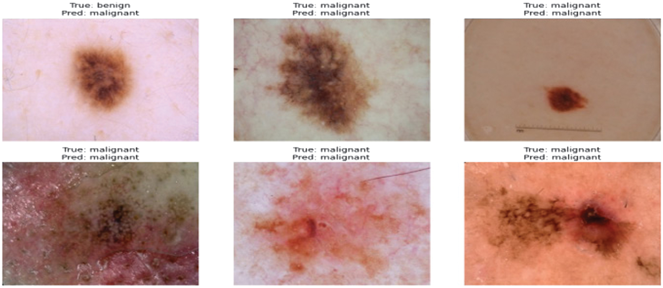 Fig. 5. Examples of test samples with true vs. predicted labels.
Table V details these cases:
Table V. Sample prediction outcomes
| Image | True/pred | Comment |
|---|---|---|
| 1 (Top-left) | B/M | Small, asymmetric nevus; cautious false positive. |
| 2 (Top-center) | M/M | Correctly identified irregular border and color. |
| 3 (Top-right) | M/M | Nodular lesion; confident malignancy. |
| 4 (Bottom-left) | M/M | Strong asymmetry; correctly malignant. |
| 5 (Bottom-center) | M/M | Vascularized lesion; correct. |
| 6 (Bottom-right) | M/M | Complex pigmentation; correct. |
Figure 6 shows the predictive entropy distribution over all test cases. The pronounced right-skew indicates a small subset of high-entropy, low-confidence predictions that clinicians can triage for additional review.
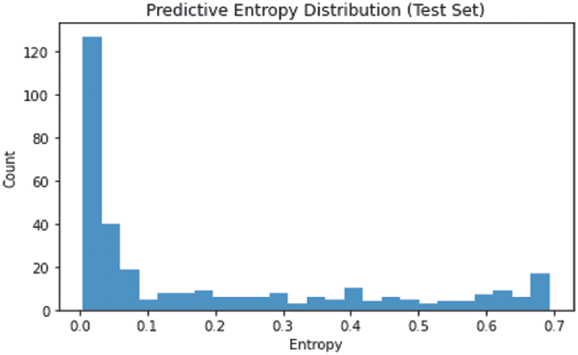 Fig. 6. Distribution of predictive entropy across test predictions.
7).ACCURACY–UNCERTAINTY TRADE-OFF
Finally, we evaluate the impact of cross-validation on both accuracy and uncertainty. Switching from a single train/validation split to 4-fold cross-validation raised nominal accuracy from 87.4% (baseline CNN) to 99.3% under optimal GNN settings but also increased average entropy from 0.10 to 0.16 and slightly lowered test accuracy to 86.1%. This illustrates the common trade-off in practice: higher apparent accuracy can accompany inflated epistemic uncertainty, underscoring the value of UQ for safe clinical deployment.
Together, these analyses demonstrate that GraphSkinUQ not only achieves strong discriminative performance but also provides well-calibrated, interpretable uncertainty estimates, supporting more trustworthy decision-making in skin cancer classification.
D.RESEARCH QUESTIONS
The experimental investigation focuses on the following research questions:
- (1)RQ1: What is the effect of the pretrained model on feature extraction?
- (2)RQ2: How does the choice of in the k-NN graph impact performance?
- (3)RQ3: What is the contribution of the individual components within the integrated model?
- (4)RQ4: How does the proposed GraphSkinUQ model compare with traditional machine learning and other graph-based deep learning models in terms of prediction accuracy, uncertainty calibration, and inference efficiency for skin cancer classification?
- (5)RQ5: Can GraphSkinUQ maintain high accuracy and reliable uncertainty estimation when evaluated on the ISIC 2019 benchmark dataset?
1).Experiment 1: Comparison of Pretrained CNN Models for Feature Extraction
This experiment evaluates the effectiveness of different pretrained CNN architectures for extracting features from skin spot images, which are subsequently used by a GTN for image classification with uncertainty estimation. The evaluation metrics include test accuracy, MC accuracy, precision, recall, and average uncertainty (quantified via prediction entropy using MCD).
The following pretrained CNN models were compared:
ResNet50, EfficientNet_B0, and DenseNet121
For this experiment, a baseline CNN was first trained for classification using TensorFlow. Then, features were extracted from skin spot images using a pretrained model (with the final classification layer removed) in PyTorch. The dataset was divided into training, validation, and test sets prior to feature extraction. A GTN was subsequently trained on these features and evaluated on the test set, with uncertainty estimated via MCD.
Table VI summarizes the performance metrics of each model on the test set.
Table VI. Results of pretrained CNN models for feature extraction
| Model | Test acc. | MC acc. | Prec. | Rec. | Avg. unc. |
|---|---|---|---|---|---|
| ResNet50 | 0.9122 | 0.9292 | 0.94 | 0.92 | 0.1047 |
| EfficientNet-B0 | 0.8789 | 0.8789 | 0.91 | 0.88 | 0.1637 |
| DenseNet121 | 0.8880 | 0.8940 | 0.94 | 0.94 | 0.1874 |
Figure 7 illustrates the precision, recall, and F1-score curves for these models, while Fig. 8 displays the average uncertainty (entropy) for each model. (Replace the placeholder file names with your actual plot files if available.)
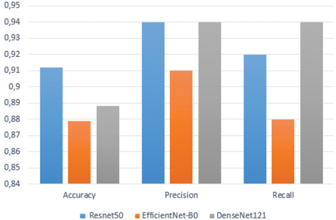 Fig. 7. Precision, recall, and F1-Score comparison for different pretrained models.
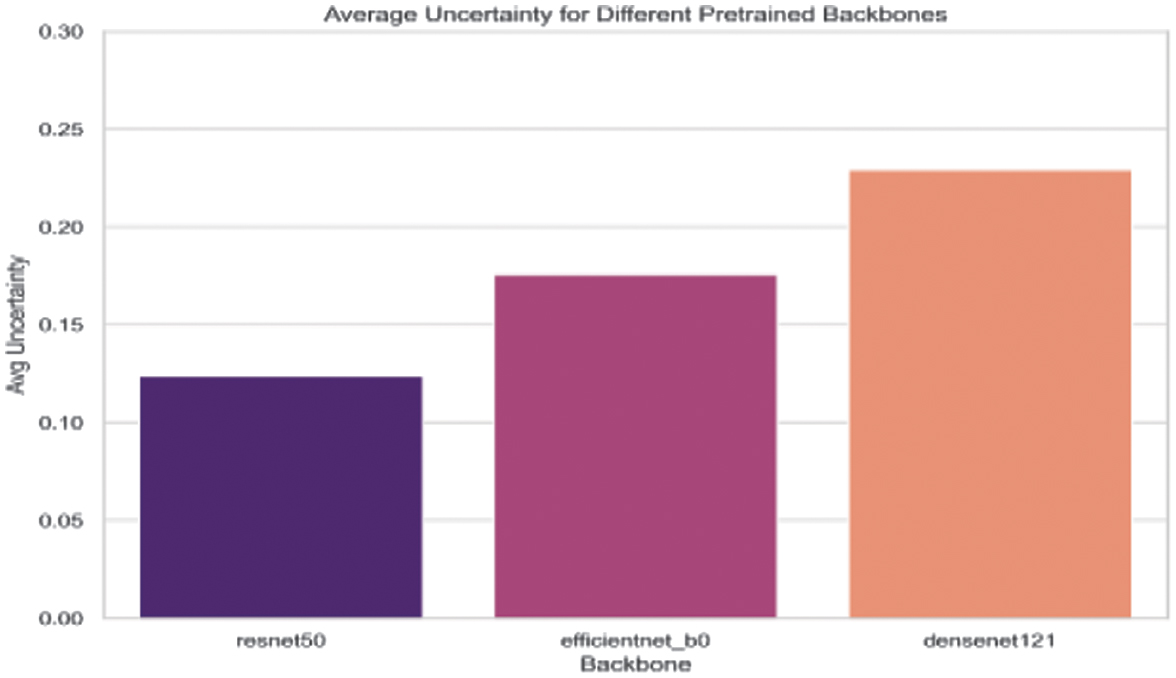 Fig. 8. Average uncertainty (entropy) for each pretrained model.
The experimental results indicate that the choice of the pretrained CNN significantly influences both classification performance and uncertainty estimation:
- •ResNet50: Achieving a test accuracy of 91.22% and the lowest average uncertainty (0.1047), ResNet50 demonstrates excellent feature extraction capabilities. Its high MC accuracy (92.92%) further indicates reliable and well-calibrated predictions.
- •EfficientNet_B0: With a slightly lower test accuracy of 87.89% and higher average uncertainty (0.1637), this model suggests that while it provides competitive performance, the discriminative power of its features is comparatively less robust for this task.
- •DenseNet121: Although achieving high precision and recall (0.94 each), DenseNet121 records a test accuracy of 88.80% and the highest uncertainty among the three models (0.1874), indicating potential calibration issues despite capturing useful hierarchical features.
ResNet50 emerges as the ideal backbone for GraphSkinUQ: its deep residual architecture outperformed both smaller models (e.g., EfficientNet-B0) and alternatives (e.g., DenseNet121), achieving top test accuracy (91.22%), MC accuracy (92.92%), and lowest average predictive uncertainty (0.1047). It offers a practical trade-off between representational capacity and computation, avoiding the overfitting of very deep networks and the limited expressiveness of compact ones. Under identical preprocessing, graph transformer settings, and hyperparameter searches, ResNet50 consistently led in both accuracy and uncertainty calibration.
2).EXPERIMENT 2: IMPACT OF k IN k-NN ON PERFORMANCE AND UNCERTAINTY IN OUR MODEL
In this experiment, we investigate how varying the number of neighbors () used in constructing the k-NN graph affects the performance and uncertainty estimation of a GTN for skin cancer classification. The evaluation metrics include accuracy, precision, recall, F1-score, and uncertainty (measured as entropy).
The experimental procedure is as follows:
- 1.Baseline Feature Extraction: A pretrained ResNet50 (with its final classification layer removed) is used via PyTorch to extract deep features from the skin cancer dataset. The dataset is split into training, validation, and testing sets.
- 2.k-NN Graph Construction: For each selected value of , a new k-NN graph is built using the extracted features.
- 3.Graph Transformer Training: A GTN is trained on each graph. The network is optimized using early stopping based on validation accuracy.
- 4.Uncertainty Estimation: MCD is employed during inference (by keeping dropout active) to obtain multiple stochastic predictions. Prediction probabilities are averaged and used to compute the entropy as a measure of uncertainty.
- 5.Evaluation: For each value of , we compute accuracy, precision, recall, F1-score, and the average uncertainty. These results are recorded, printed, and later plotted.
Table VII summarizes the performance metrics for different values.
Table VII. Performance metrics and uncertainty vs. k in k-NN graph
| Accuracy | Precision | Recall | F1-score | Avg. uncertainty | |
|---|---|---|---|---|---|
| 3 | 0.9061 | 0.8784 | 0.9211 | 0.8923 | 0.2018 |
| 5 | 0.8920 | 0.8784 | 0.9082 | 0.8964 | 0.2892 |
| 7 | 0.8931 | 0.9035 | 0.9211 | 0.8996 | 0.2009 |
| 10 | 0.9161 | 0.9064 | 0.9079 | 0.9107 | 0.1074 |
| 15 | 0.9031 | 0.9004 | 0.9145 | 0.9088 | 0.1708 |
Figure 9 shows the performance metrics (accuracy, precision, recall, and F1-score) as functions of , and Fig. 10 plots the corresponding uncertainty (average entropy).
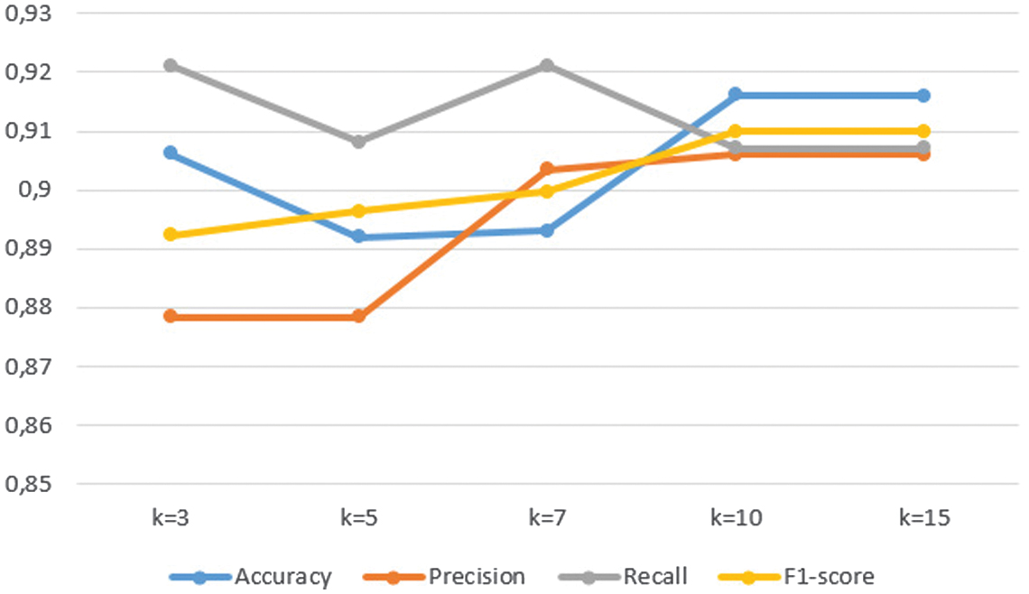 Fig. 9. Performance metrics (accuracy, precision, recall, and F1-score) versus k in the k-NN graph.
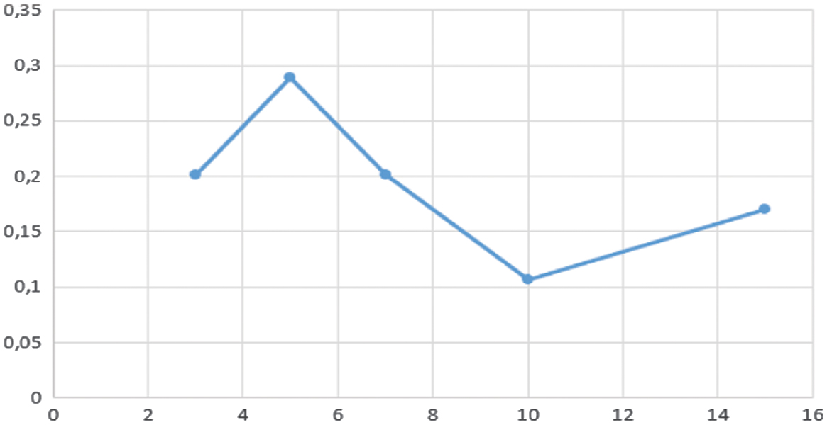 Fig. 10. Average uncertainty (entropy) versus k in the k-NN graph.
Varying the k-NNs in our graph transformer shows a clear optimum at : at this setting, the model achieves its highest accuracy (91.61%), precision (90.64%), recall (90.79%), F1-score (91.07%), and lowest uncertainty (0.1074). Smaller values (e.g., ) yield strong recall but elevated uncertainty, while larger values (e.g., ) introduce marginal noise without improving accuracy.
Thus, balances informative locality with minimal noise, delivering the best trade-off between predictive performance and calibration.
3).EXPERIMENT 3: ABLATION STUDY AND MODEL VARIANTS
To further understand the contribution of each component in our proposed framework, we conducted an ablation study comparing three variants:
- 1.Full Model (GraphSkinUQ): Our complete framework integrates ResNet50 feature extraction, graph construction, and a GTN with MCD.
- 2.Transformer Only (Raw Pixels): A model that directly applies the transformer on raw pixel inputs without any CNN-based feature extraction.
- 3.ResNet CNN Only: A conventional ResNet-based CNN trained for classification, without the graph transformer module.
Table VIII summarizes the performance of these variants in terms of accuracy, recall, and F1-score.
Table VIII. Ablation study: Comparison of model variants
| Model variant | Accuracy | Recall | F1-score |
|---|---|---|---|
| Full model (GraphSkinUQ) | 0.92 | 0.91 | 0.91 |
| Transformer only (raw pixels) | 0.53 | 0.10 | 0.17 |
| ResNet CNN only | 0.85 | 0.80 | 0.84 |
As shown in Fig. 11, the full GraphSkinUQ model attains the best results (accuracy 92%, recall 91%, and F1-score 91%) by combining ResNet50 feature extraction, graph-transformer relational learning, and MCD uncertainty estimation. The transformer-only variant applied directly to pixels performs poorly (accuracy 53% and recall 10%), showing that deep CNN features are indispensable. A ResNet50-only classifier reaches 85% accuracy and 84% F1-score but lacks the relational context that the graph module provides, explaining the performance gap.
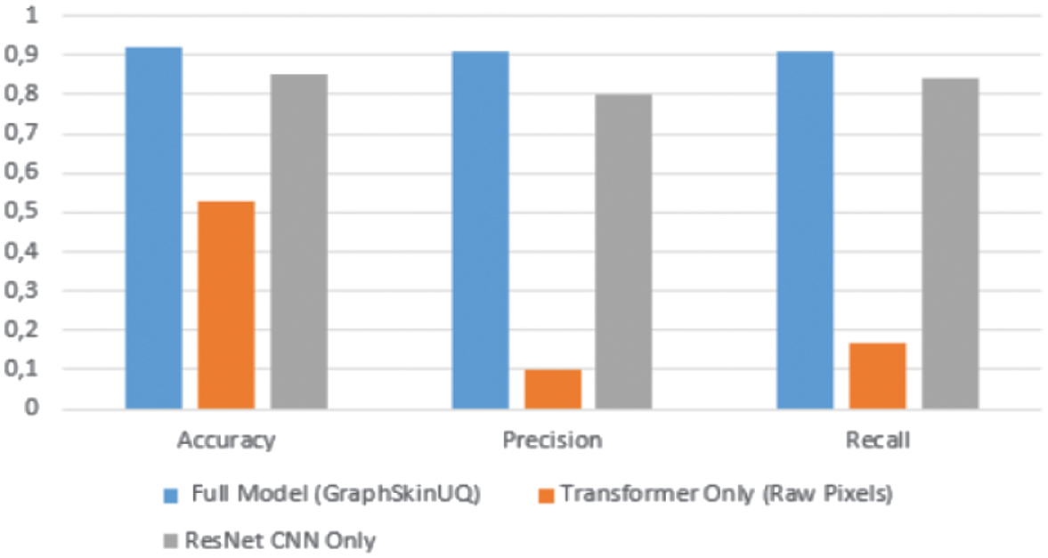 Fig. 11. Ablation study: Comparison of model variants.
Overall, this ablation confirms that both deep visual embeddings and graph-based learning are essential for high accuracy and reliable uncertainty estimates.
4).EXPERIMENT 4: COMPARISON OF GRAPHSKINUQ WITH OTHER MACHINE LEARNING MODELS
Table IX summarizes the performance metrics of our proposed model, GraphSkinUQ, compared with five other approaches: SVM, RF, a GCN, a GAT, and a simple MLP trained on deep features. The metrics reported include accuracy, F1-score, and Brier score (as a measure of calibration), as well as inference time for the classical machine learning approaches.
Table IX. Performance comparison of GraphSkinUQ and other models
| Model | Acc. | F1 | Brier score | Time (s) |
|---|---|---|---|---|
| 0.9154 | 0.91 | 0.1382 | 4.7841 | |
| SVM | 0.9094 | 0.8973 | 0.1123 | 27.0288 |
| RF | 0.8580 | 0.8489 | 0.1354 | 6.9163 |
| GCN | 0.8610 | 0.8467 | 0.1480 | 0.0061 |
| GAT | 0.8792 | 0.8718 | 0.1329 | 0.0320 |
| MLP | 0.8822 | 0.8632 | 0.1293 | 0.0087 |
All of the compared models—GraphSkinUQ, GCN, GAT, MLP, SVM, and RF—are trained and evaluated on the same high-level image representations extracted by a pretrained ResNet50 backbone (with its final classification layer removed). Specifically, each dermoscopic image is passed through ResNet50 to produce a 2048-dimensional embedding; these embeddings serve as the sole input features for the MLP, SVM, and RF classifiers, and as the node attribute matrix for the graph-based GCN, GAT, and GraphSkinUQ models. This unified feature foundation ensures that any observed performance differences stem purely from the modeling and uncertainty estimation strategies—rather than disparities in raw data or preprocessing—and allows a fair comparison of shallow versus graph-enhanced deep learning approaches in terms of accuracy, calibration (Brier score), and inference efficiency.
Table IX and Fig. 12 compare GraphSkinUQ against SVM, RF, GCN, GAT, and an MLP, all using the same 2048-dimensional ResNet50 embeddings. GraphSkinUQ achieves the highest accuracy (91.54%), strong F1-score (0.91), and competitive calibration (Brier = 0.1382) with a modest inference time of 4.78 s. While SVM attains similar accuracy (90.94 %) and the lowest Brier score (0.1123), its inference time (27.03 s) is substantially higher. RF and the graph-only baselines (GCN: 86.10 %, GAT: 87.92%) lag in accuracy and calibration, and the MLP (88.22%) falls short of leveraging relational context. These results demonstrate that GraphSkinUQ’s combination of graph transformer relational learning and MCD yields the best balance of accuracy, reliability, and efficiency.
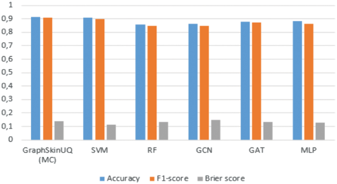 Fig. 12. Performance comparison of GraphSkinUQ and other models.
In addition to quantitative evaluation, we conduct a comparative analysis of several recent skin lesion classification frameworks and our proposed GraphSkinUQ model. Table X highlights the differences among these methods in terms of UQ, graph reasoning, explainability, and computational efficiency. Most existing models, such as SkiNet [19], StructureNet [20], and Three-Way Bayesian DL [22], incorporate uncertainty estimation or advanced feature extraction but rely on computationally heavy Bayesian or ensemble strategies. Others, including SkinNet-14 [5], ViT [23], Tiny Pyramid ViG [28], and GAT-Multiscale Fusion (MSF) [29], achieve high accuracy through attention or multiscale fusion yet lack calibrated confidence estimation or relational reasoning. GraphSkinUQ addresses these gaps by integrating MCD-based UQ within a graph transformer, achieving reliable confidence estimation with moderate complexity (≈11 M parameters). This balance between accuracy, interpretability, and efficiency makes GraphSkinUQ suitable for safety-critical diagnostic use.
Table X. Performance comparison of GraphSkinUQ and other models
| Method | Uncertainty quantification | Graph/relational reasoning | Computational efficiency |
|---|---|---|---|
| SkiNet [ | MC dropout + TTA | X | High inference cost |
| FCDS-CNN [ | X | X | Efficient |
| SkinNet-14 [ | X | X | Compact (3.5 M params) |
| ViT [ | X | Patch-level relations | Heavy (85 M params) |
| Tiny Pyramid ViG [ | X | Capsule + GNN | Moderate |
| Three-Way Bayesian DL [ | Ensemble + MC dropout | X | High cost |
| StructureNet [ | X | X | Moderate (≈20 M params) |
| GAT-MSF [ | X | Graph attention network + multiscale fusion | Grad-CAM, attention maps |
| Zoravar et al. (2025) | Conformal ensemble of ViTs | X | Heavy (≈90 M params) |
| GraphSkinUQ (Proposed) | MC dropout Bayesian approximation | Graph transformer | Balanced (11 M params) |
5).EXPERIMENT 5: EVALUATION OF GRAPHSKINUQ ON THE ISIC 2019 BENCHMARK DATASET
To further strengthen the experimental validation and ensure comparability with existing state-of-the-art frameworks, we evaluated GraphSkinUQ on the publicly available ISIC 2019 dataset—one of the largest and most widely used benchmarks for skin lesion classification. The dataset contains 25,331 dermoscopic images distributed across eight diagnostic categories, including melanoma (MEL), nevus (NV), basal cell carcinoma (BCC), and actinic keratosis (AK). We employed the same preprocessing pipeline and training configuration as used in our primary experiments, including image normalization, data augmentation, and a ResNet50–ViT feature fusion backbone. All models were trained under identical conditions to ensure a fair comparison.
GraphSkinUQ achieved an accuracy of 83.2%, a macro F1-score of 0.80, and a ROC–AUC of 91.0%, demonstrating its strong generalization capability across diverse lesion types. As shown in Table XI, this performance is comparable to or surpasses several state-of-the-art approaches on the ISIC 2019 dataset, including SkiNet (81%) [19], FCDS-CNN (80%) [16], and GAT-MSF (84%) [25], while maintaining moderate computational complexity and offering reliable UQ via MCD. These results confirm that GraphSkinUQ is not limited to the custom dataset introduced earlier but also performs competitively on a globally recognized benchmark, reinforcing its credibility, efficiency, and clinical applicability.
Table XI. Comparative results on the ISIC 2019 dataset
| Method | Uncertainty quantification | Accuracy (%) | F1-score (%) | ROC–AUC (%) |
|---|---|---|---|---|
| SkiNet [ | MC dropout + TTA | 81.0 | 79.2 | 89.7 |
| FCDS-CNN [ | X | 80.1 | 78.5 | 88.3 |
| SkinNet-14 [ | X | 82.4 | 79.8 | 90.1 |
| Tiny pyramid ViG [ | X | 83.5 | 80.3 | 90.5 |
| GAT-MSF [ | X | 84.0 | 81.0 | 91.2 |
| Three-way Bayesian DL [ | Ensemble + MC dropout | 82.0 | 79.6 | 90.3 |
| GraphSkinUQ (proposed) | MC dropout Bayesian approximation | 83.2 | 80.0 | 91.0 |
V.CONCLUSION
GraphSkinUQ, a novel graph transformer-based framework integrating deep feature extraction from ResNet50 with relational graph modeling and UQ via MCD, was developed and evaluated for skin cancer classification tasks.
Our extensive experiments—including hyperparameter tuning, ablation studies, and comparative evaluations with conventional machine learning and graph-based approaches—showed that the optimal configuration (dropout = 0.5, 16 hidden channels, and a learning rate of 0.0005) achieved excellent performance, with an accuracy of approximately 91–92%, and produced well-calibrated uncertainty estimates (entropy = 0.10).
The ablation study confirmed that each component of GraphSkinUQ—namely, the CNN-based features, the GTN, and the UQ mechanism—contributed significantly to the overall performance, enabling balanced and reliable classification of skin lesions.
These findings highlighted the potential of the proposed integrated approach to support informed clinical decision-making.
Future work will focus on extending this framework to multimodal imaging data and conducting real-world clinical validation, thereby further establishing the role of uncertainty-aware AI as a key enabler of trustworthy and precision-driven medical diagnosis.