I.INTRODUCTION
Diabetes mellitus is an intricate metabolic disorder that manifests in high blood glucose levels [1]. This mellitus presents challenges that lead to serious complications, including cardiovascular diseases and failure of the kidneys [2]. The World Health Organization (WHO) states that the affliction affects society beyond the individual suffering. Moreover, there has been a drastic rise in case numbers in the past few decades, particularly in low- and middle-income countries [3]. As illustrated in Fig. 1, the rise in prevalence in these areas emphasizes the need for early detection and management [4].
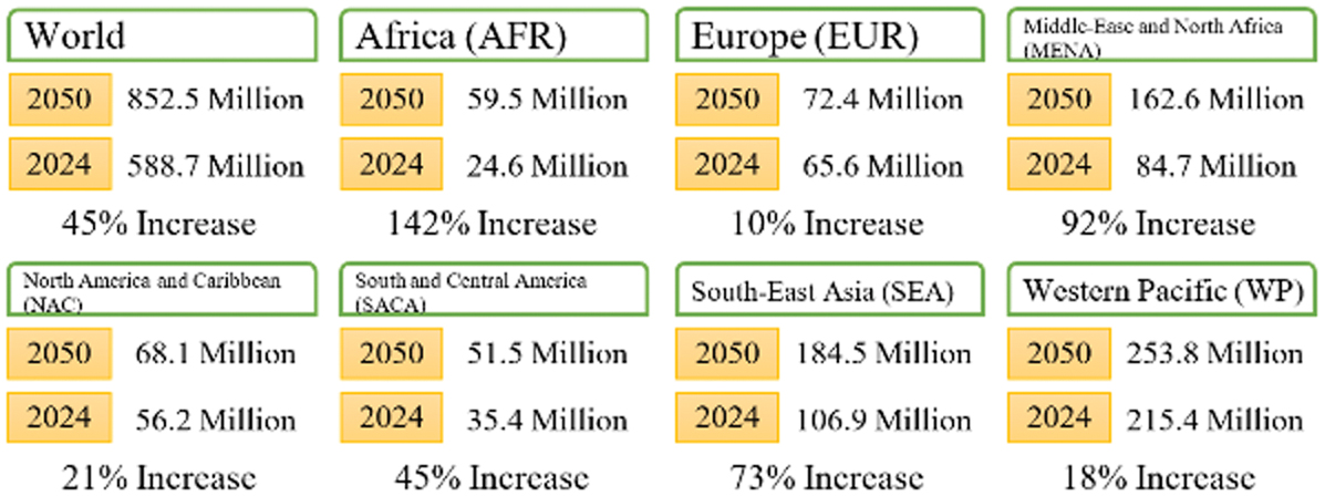 Fig. 1. Diabetes cases around the world in 2024 [4].
To help confront this public health crisis, it is essential to detect and address the development of diabetes at an early stage. By beginning treatment before the onset of possible complications, more lives can be preserved, all with the goal of improving their quality of life and keeping those at risk healthy enough to live longer. Early diagnosis can improve outcomes in diabetes before it has progressed enough to cause serious complications or damaging effects on the patient or the American healthcare system. The result would be benefits for all of them, including better-quality diabetes management and substantial savings in costs and lost productivity [5].
Machine learning can develop predictive models identifying the individuals at high risk based on clinical and demographic data; hence, it offers an automated, efficient, and reliable alternative to classic approaches [6]. Supervised machine learning is the training of algorithms on labeled datasets with known outputs [7–9]. The models are then used for predicting diabetes [10].
Although machine learning technologies provide a reliable approach for diabetes prediction, there are still a few challenges, including (1) Data Quality and Availability: Clinical and demographic datasets are generally small, with much of the data either missing or excessively noisy [11]. Limited sample sizes and incomplete records may reduce the accuracy and generalizability of the models. In addition, using small datasets with very complex models can lead to overfitting, where the algorithm performs well on the training data but fails to generalize to unseen data [12]. (2) Class Imbalance: The number of non-diabetic cases often greatly outweighs diabetic ones. This imbalance can lead to biased models that are overly focused on the majority class and therefore under-sensitive to high-risk individuals. (3) Researching features of varying importance: Identifying the most relevant features for diabetes prediction is crucial and challenging. Irrelevant or redundant features may negatively impact model performance, while missing an important feature may result in poor predictive performance [13].
Unsupervised learning is one of the most powerful tools for discovering patterns and relationships in unlabeled data. Their power of dimensionality reduction, the addressing of redundancies, and further preprocessing of rights and data render their utility across a spectrum of domains. However, the lack of labeled outputs, reliance on domain expertise, sensitivity to noise, and parameter choices have all revealed certain limitations. Thus, unsupervised methods tend to perform well when combined with other techniques, such as semi-supervised learning and/or feature engineering, for better usability and robust applicability [14].
The significance of combining both techniques lies in leveraging their strengths. Supervised methods excel at direct predictions, while unsupervised methods offer insights into data structure and can enhance feature engineering, improve model generalization, and detect anomalies or subgroups in datasets. The PIMA dataset includes clinical attributes like glucose levels, BMI, and insulin concentrations, which are used to train predictive models [15]. However, one major drawback is the small size of datasets like PIMA and the class imbalance, where there are significantly more non-diabetic cases than diabetic ones. This imbalance can lead to biased models, reduced sensitivity to positive cases, and overfitting. Traditional methods often struggle to perform well under these conditions, which limits their effectiveness in real-world applications. As such, a hybrid approach is required to improve the performance of the diabetes prediction task [16].
In this study, clustering is integrated with classification, where the clustering stage groups patients into homogeneous clusters based on health attributes such as glucose, BMI, and age. This stratification enables each classifier to learn more meaningful intra-cluster relationships, improving predictive sensitivity for minority diabetic cases. Additionally, feature selection is applied to eliminate irrelevant or redundant variables, reducing computational load and enhancing interpretability.
The structure of this paper is as follows: Section II presents a literature review that provides an overview of existing diabetes prediction models. Section III presents a detailed explanation of the hybrid framework, including data preprocessing, feature selection, and the integration of supervised and unsupervised techniques. Section IV presents an evaluation of the proposed approach. Section V discusses the results. Finally, the conclusion and the future work are presented in Section VI.
II.RELATED WORK
The prediction of diabetes has become a significant area of research in machine learning, given its significant impact on global health. Numerous studies have used both supervised and unsupervised learning methods to improve prediction accuracy while addressing issues such as limited datasets, class imbalance, and complex features [17].
A.SUPERVISED MACHINE LEARNING FOR DIABETES PREDICTION
Supervised machine learning has become a highly effective method for predicting diabetes. Various classification algorithms, such as Decision Tree (DT), Random Forests (RF), Support Vector Machine (SVM), and Logistic Regression (LR), have achieved impressive results when applied to structured datasets, including the PIMA Indian Diabetes Dataset.
An early approach by Sisodia and Sisodia [18] compared multiple algorithms, including DT, Naïve Bayesian (NB), and SVM, to assess their effectiveness in diabetes classification. Their findings highlighted that NB achieved the best accuracy of 76.3% accuracy with 10-fold cross-validation. Wei et al. [19] evaluated Deep Neural Networks (DNN), LR, DT, NB, and SVM classifiers for diabetes prediction. The proposed framework consists of preprocessing the dataset through imputation, normalization, and feature selection using Principal Component Analysis (PCA) and Linear Discriminant Analysis (LDA), and classifying using the resulting features. Their study reported that DNN performed the best, achieving 77.86% accuracy with 10-fold cross-validation.
Kibria et al. [20] used LR, SVM, Artificial Neural Networks (ANN), RF, Adaptive Boosting (AB), and eXtreme Gradient Boosting (XGB) classifiers to predict diabetes using the PIMA dataset. Missing values were imputed, after which the dataset was normalized, followed by feature selection and oversampling. The results showed that ensemble learning achieved the best accuracy of 89% with 5-fold cross-validation. Simaiya et al. [21] used K-Nearest Neighbors (KNN), NB, DT, RF, JRip, and SVM in a three-layer framework, with layers consisting of 3, 2, and 1 classifier(s), respectively. Feature selection and oversampling were used prior to the classification stage. The results showed that the proposed framework achieved a precision of 78.4% with 10-fold cross-validation.
Marzouk et al. [22] used ANN, KNN, LR, NB, DT, RF, SVM, and Gradient Boosting (GBoost) classifiers. The preprocessing stage consists of handling missing values and normalizing the data. The results showed that ANN achieved the highest accuracy of 81.7% with 5-fold cross-validation. Yadav and Nilam [23] used KNN, DT, SVM, and RF. The preprocessing stage consists of normalization. The results showed that KNN achieved the best performance with an accuracy of 80%.
Reza et al. [24] used an enhanced kernel SVM with missing-value imputation, implemented normalization, removed outliers, and oversampled. The results showed that SVM achieved an accuracy of 85.5% 10-fold cross-validation. Perdana et al. [25] used KNN with various k values to improve performance. The results showed that 22 achieved the best performance, with an accuracy of 83.12% on a 90%–10% train-test split. Al-Dabbas [26] used SVM, RF, and XGB to fill in missing values and oversample. The results showed that XGB achieved the best accuracy of 91% using a 90%–10% train-test split.
In summary, classification-based diabetes prediction is robust and applicable to both structured and unstructured datasets. However, these methods often face challenges related to overfitting and generalization, especially when dealing with small datasets or imbalanced class distributions. Techniques such as normalization, feature selection, oversampling, and cross-validation have been proposed to mitigate these issues. Nevertheless, their performance is often limited by the quality and quantity of available data, and they can struggle to uncover deeper, nonlinear patterns within the dataset [27]. A summary of these findings is presented in Table I.
Table I. Supervised ML-based diabetes prediction
| Ref. | Preprocessing | Classifiers | CV | Accuracy | ||||||||||||||||
|---|---|---|---|---|---|---|---|---|---|---|---|---|---|---|---|---|---|---|---|---|
| H | N | R | S | O | 1 | 2 | 3 | 4 | 5 | 6 | 7 | 8 | 9 | 10 | 11 | 12 | 13 | |||
| Sisodia and Sisodia [ | √ | √ | √ | 10 | 76.3% | |||||||||||||||
| Wei et al. [ | √ | √ | √ | √ | √ | √ | √ | 10 | 77.86% | |||||||||||
| Kibria et al. [ | √ | √ | √ | √ | √ | √ | √ | √ | √ | √ | √ | 5 | 89% | |||||||
| Simaiya et al. [ | √ | √ | √ | √ | √ | √ | √ | 10 | 78.4% | |||||||||||
| Marzouk et al. [ | √ | √ | √ | √ | √ | √ | √ | 5 | 83.1% | |||||||||||
| Yadav and Nilam [ | √ | √ | √ | √ | √ | √ | √ | √ | √ | √ | 10 | 81.7% | ||||||||
| Reza et al. [ | √ | √ | √ | √ | 10 | 85.5% | ||||||||||||||
| Perdana et al. [ | √ | √ | χ | 83.12% | ||||||||||||||||
| Al-Dabbas [ | √ | √ | √ | √ | √ | √ | √ | √ | χ | 91% | ||||||||||
Preprocessing, H:
B.UNSUPERVISED LEARNING FOR DIABETES ANALYSIS
Unsupervised learning has applications in healthcare, especially for analyzing complex datasets in diabetes research. In contrast to supervised methods that depend on labeled data, unsupervised techniques reveal hidden patterns and relationships within the data without needing explicit outcome labels. These approaches are especially valuable for categorizing patients, identifying at-risk groups, and discovering new insights from diabetes datasets. Unsupervised learning was not exhaustively used to predict diabetes. As such, Cao et al. [28] used k-means to generate clusters and classify new instances based on the distance to those clusters. The results were evaluated using a combination of PIMA and Medical Information Mart for Intensive Care (MIMIC) datasets. The critical challenge of unsupervised machine learning is that evaluating its results remains subjective and requires domain expertise to interpret the identified clusters and patterns accurately.
C.HYBRID APPROACHES
Hybrid models combine the predictive capabilities of supervised learning with the exploratory power of unsupervised methods, enabling better pattern recognition, noise reduction, and anomaly detection. Edeh et al. [29] used RF, DT, SVM, and NB classification algorithms and employed a technique for missing-values imputation and outlier removal based on unsupervised learning. The results showed that SVM achieved the best performance, with an accuracy of 83.1% based on an 80%–20% train-test split. Chang et al. [30] used NB, RF, and DT classifiers with k-means clustering for feature selection. The preprocessing stage consists of imputing missing values and selecting features. The results showed that RF achieved the best accuracy of 86.24% with a 70%–30% train-test split. A summary of the hybrid approaches is given in Table II.
Table II. Hybrid-based diabetes prediction
| Ref. | SML | UML | CV | Accuracy |
|---|---|---|---|---|
| Edeh et al. [ | RF, DT, SVM, and NB | Outlier removal | χ | 83.1% |
| Chang et al. [ | DT | Feature selection | χ | 86.24% |
D.ADDRESSING LIMITATIONS IN CURRENT RESEARCH
Although significant progress has been made in diabetes prediction, several limitations persist. Most existing studies focus on improving prediction accuracy but neglect model scalability and interpretability, which are critical for real-world healthcare applications. Additionally, reliance on a single dataset, such as PIMA, limits the generalizability of results, as it primarily represents a specific population with unique characteristics. Hybrid methods, while effective, often introduce implementation complexity and require a fine balance between supervised and unsupervised components.
III.THE PROPOSED FRAMEWORK
A hybrid machine learning framework combining supervised and unsupervised learning techniques is proposed to improve diabetes prediction using the PIMA Indian Diabetes Dataset. The framework consists of several stages, as illustrated in Fig. 2, including data preprocessing, feature selection, hybrid modeling, and evaluation. The proposed approach aims to address challenges such as class imbalance, limited dataset size, and feature redundancy while leveraging the complementary strengths of supervised and unsupervised techniques.
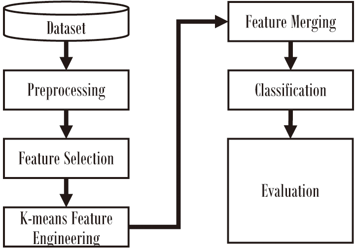 Fig. 2. The proposed approach.
A.DATASET
The PIMA Indian Diabetes dataset is a widely used benchmark in diabetes prediction studies. It contains 768 samples with 8 numerical features, each representing a female of PIMA Indian heritage aged 21 years or older. Table III provides example entries from the dataset to clarify structure and labeling. The dataset comprises eight numerical attributes, including the number of pregnancies, glucose levels, blood pressure, skin thickness, insulin levels, body mass index (BMI), diabetes pedigree function (a measure of genetic influence), and age, as summarized in Table IV. Notably, some attributes have missing or zero values, particularly insulin and skin thickness, which can challenge model training and require preprocessing. The target variable indicates whether the individual has diabetes (1) or not (0), with 500 non-diabetic (0) and 268 diabetic (1) instances, showing a slight class imbalance. Table V summarizes the characteristics of the PIMA dataset. This dataset serves as a foundation for analyzing risk factors associated with diabetes while providing opportunities to address challenges such as missing data and class imbalance [31].
Table III. Part of the PIMA dataset for illustration purposes
| Pregnancies | Glucose | BP | BMI | Insulin | Age | Pedigree | Outcome |
|---|---|---|---|---|---|---|---|
| 2 | 120 | 70 | 33.6 | 85 | 27 | 0.35 | 0 |
| 8 | 183 | 64 | 32.9 | 210 | 37 | 0.67 | 1 |
Table IV. The risk factors of diabetes as reported in the PIMA dataset
| Feature | Description | Range |
|---|---|---|
| Pregnancies | Number of pregnancies | 0–17 |
| Glucose | Plasma glucose concentration after 2 hours | 0–199 |
| Blood pressure | Diastolic blood pressure (mmHg) | 0–122 |
| Skin thickness | Triceps skinfold thickness (mm) | 0–99 |
| Insulin | Serum insulin (U/ml) | 0–846 |
| BMI | Body mass index (weight in kg/m2) | 0–67.1 |
| Diabetes pedigree function | Diabetes likelihood based on family history. | 0.078–2.42 |
| Age | Age of the person (years) | 21–81 |
| Outcome | Diabetes status (1 = positive, 0 = negative) | Binary |
Table V. The characteristics of the PIMA dataset
| Characteristic | Value |
|---|---|
| Number of samples | 768 |
| Number of features | 8 (all numerical) |
| Target variable | Binary (0 = no diabetes, 1 = diabetes) |
| Non-diabetic instances | 500 |
| Diabetic instances | 268 |
| Missing data | Represented as zeros in certain features |
| Features with missing data | Insulin, skin thickness, blood pressure, BMI, glucose |
B.DATA PREPROCESSING
Data preprocessing prepares the PIMA dataset for modeling. This includes handling missing values. In this process, the missing values, which in this case are zeros, are replaced using median imputation. The zero value is an unreasonable value across the dataset used, including features such as glucose and insulin levels. Besides, outliers are also replaced with median values.
C.FEATURE SELECTION
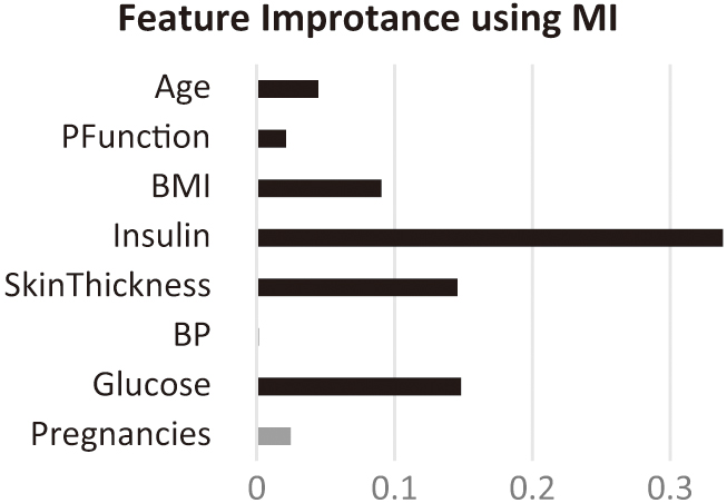
Feature selection is crucial for reducing dimensionality, eliminating irrelevant features, and improving model performance. The proposed framework employs Mutual Information (MI) to assess feature-target variable dependencies and select the most relevant features for diabetes prediction. Selecting the significant features is implemented by calculating the MI score for each feature and then selecting the features with the highest MI scores.
D.CLUSTERING
The first stage of the hybrid framework applies K-means clustering to group similar patient records based on feature similarity. The optimal number of clusters (k) was selected experimentally using the Elbow method and the Silhouette coefficient, which both indicated two distinct patient clusters. This small number of clusters provided a good trade-off between interpretability and separation strength. Increasing k beyond 2 led to small, unstable clusters and degraded classifier performance. Each patient record’s cluster label was appended as an additional feature to the dataset, effectively encoding unsupervised structure for downstream classification.
E.CLASSIFICATION STAGE
The processed dataset, enriched with cluster labels and reduced by feature selection, was evaluated using 13 classifiers, including SVM, KNN, DT, RF, Neural Networks (ANN), AB, Gaussian NB, Quadratic Discriminant Analysis (QDA), Skope Rules (JRip), XGB, Gradient Boosting (GB), DNN, and LR.
F.HYBRID MODELING APPROACH
The core of the proposed work is the integration of supervised and unsupervised learning methods to improve predictive performance.
- •Unsupervised Component: K-means clustering is applied to group patients based on their clinical and demographic features. These clusters are used to identify latent patterns in the data that hold patients with varying risk levels.
- •Supervised Component: Multiple classifiers are used to predict diabetes risk. The unsupervised clusters are incorporated as additional features or used for stratified training to improve model sensitivity and accuracy.
The hybrid approach is implemented following the steps:
- 1.The number of clusters is identified using the Elbow method.
- 2.K-means clustering is applied to the preprocessed dataset to generate patient clusters.
- 3.The K-means-generated cluster label is used as an additional feature.
- 4.The supervised algorithm, using one of the classification algorithms, is applied to the enhanced dataset.
IV.EXPERIMENTAL RESULTS
All experiments were conducted in Python 3.9 on an Intel Core i7 (1.8 GHz) system using the scikit-learn and XGB libraries. Each experiment was repeated five times with different random seeds to ensure reproducibility. Statistical significance was tested using the Wilcoxon signed-rank test (α = 0.05) to confirm whether improvements were non-random.
A.EXPERIMENTAL SETTINGS
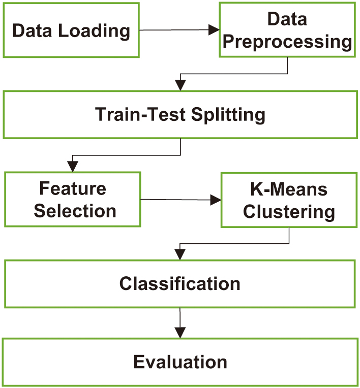
The overall workflow of the proposed system is illustrated in Fig. 3, which can be described as follows:
- 1.Load the PIMA Indian Diabetes Dataset.
- 2.Preprocess the dataset by handling missing values and scaling features.
- 3.Perform feature selection using MI.
- 4.Apply K-means clustering to identify patient subgroups (iterate and evaluate using the Elbow method).
- 5.Use supervised classifiers that incorporate clustering results for diabetes prediction.
- 6.Evaluate and compare model performance using standard metrics.
B.FEATURE EVALUATION
Figure 4 illustrates the MI scores of all features, highlighting the selected features for the study. According to the MI scores, blood pressure and pregnancy are eliminated.
C.EVALUATION MEASURES
The proposed approach will evaluate the accuracy, precision, recall, F1-score, and area under the receiver operating characteristic (ROC) curve (AUC), summarized in Table VI.
Table VI. Summary of the evaluation metrics
| Metric | Description | Purpose |
|---|---|---|
| Proportion of correctly predicted samples to the total samples. | Measures the overall performance of the model. | |
| The ratio of true positives to the total predicted positives (TP/(TP + FP)). | Measures the ratio of the correctly predicted positives. | |
| The ratio of true positives to the total actual positives (TP/(TP + FN)). | Measures the model’s ability to identify all positive samples. | |
| Integration of precision and recall (2 * (Precision * Recall)/(Precision + Recall)). | Provides a balance between precision and recall. | |
| The area under the receiver operating characteristic curve, which plots true positive rate vs. false positive rate. | Reflects the model’s ability to distinguish between classes across various thresholds. |
D.PARAMETER SETTINGS
All models were trained using the default hyperparameters from the scikit-learn and XGB libraries to ensure comparability and reproducibility across different classifiers. The default parameters are given in Table VII.
Table VII. Parameter settings for the classifiers
| Clas. | Parameters | Values |
|---|---|---|
| kernel, C, gamma | rbf, 1.0, scale | |
| k, weights | 5, uniform | |
| criterion, splitter | Gini, best | |
| n, criterion | 100, gini | |
| layer size, activation, solver, iteration | (100), relu, adam, 200 | |
| n, learning rate | 50, 1.0 | |
| smoothing | 1e–09 | |
| param, store | 0.0, False | |
| minNo | 1 | |
| n, depth, learning rate, subsample, colsample_bytree | 100, 6, 0.3, 1.0, 1.0 | |
| n, learning rate, depth | 100, 0.1, 3 | |
| layer size, activation, solver, iteration | (100, 50, 25), relu, adam, 200 | |
| penalty, solver, C, iteration | l2, lbfgs, 1.0, 100 |
E.EVALUATION
The experiments will evaluate the proposed model and each component individually. Table VIII summarizes the results of the classifiers without feature selection or clustering.
Table VIII. Results of the baseline model
| # | Clas. | Acc. | Prec. | Rec. | F1 | AUC |
|---|---|---|---|---|---|---|
| SVM | 0.651 | 0.000 | 0.000 | 0.000 | 0.500 | |
| KNN | 0.850 | 0.789 | 0.780 | 0.784 | 0.834 | |
| DT | 0.861 | 0.834 | 0.750 | 0.790 | 0.835 | |
| RF | 0.878 | 0.830 | 0.817 | 0.823 | 0.864 | |
| ANN | 0.813 | 0.790 | 0.631 | 0.701 | 0.770 | |
| AB | 0.866 | 0.814 | 0.799 | 0.806 | 0.850 | |
| NB | 0.766 | 0.677 | 0.627 | 0.651 | 0.733 | |
| QDA | 0.742 | 0.655 | 0.552 | 0.599 | 0.698 | |
| JRip | 0.819 | 0.679 | 0.914 | 0.779 | 0.841 | |
| XGB | 0.844 | 0.810 | 0.827 | 0.865 | ||
| GB | 0.875 | 0.828 | 0.810 | 0.819 | 0.860 | |
| DNN | 0.803 | 0.714 | 0.728 | 0.721 | 0.786 | |
| LR | 0.776 | 0.710 | 0.604 | 0.653 | 0.736 |
Among the classifiers, XGB achieved the highest accuracy of 0.882, precision of 0.844, F1-score of 0.827, and AUC of 0.865, making it the most effective classifier in the baseline model. Similarly, RF and GB achieved competitive results, demonstrating the robust performance of ensemble-based methods. In contrast, simpler classifiers like NB and QDA achieved lower precision, recall, and F1-scores, indicating limitations in handling the dataset’s complexity without further enhancements. Surprisingly, JRip showed a strong recall of 0.914, suggesting it effectively identified positive cases, albeit at the expense of precision.
Table IX summarizes the results of the classifiers in the baseline model with feature selection.
Table IX. Results of the baseline model with feature selection
| # | Clas. | Acc. | Prec. | Rec. | F1 | AUC |
|---|---|---|---|---|---|---|
| SVM | 0.654 | 1.000 | 0.007 | 0.015 | 0.504 | |
| KNN | 0.868 | 0.813 | 0.810 | 0.811 | 0.855 | |
| DT | 0.867 | 0.840 | 0.765 | 0.801 | 0.843 | |
| RF | 0.882 | 0.834 | 0.825 | 0.830 | 0.868 | |
| ANN | 0.789 | 0.717 | 0.653 | 0.684 | 0.757 | |
| AB | 0.870 | 0.821 | 0.802 | 0.811 | 0.854 | |
| NB | 0.768 | 0.694 | 0.601 | 0.644 | 0.729 | |
| QDA | 0.734 | 0.655 | 0.504 | 0.570 | 0.681 | |
| JRip | 0.823 | 0.683 | 0.918 | 0.783 | 0.845 | |
| XGB | 0.840 | 0.825 | 0.832 | 0.870 | ||
| GB | 0.840 | 0.825 | 0.832 | 0.870 | ||
| DNN | 0.763 | 0.662 | 0.657 | 0.660 | 0.738 | |
| LR | 0.762 | 0.690 | 0.575 | 0.627 | 0.718 |
Building on the baseline model without feature selection (Table VIII), Table IX presents the performance of classifiers after incorporating MI-based feature selection. This refinement generally improved model performance, particularly for ensemble methods and complex classifiers, by reducing irrelevant or redundant features, which enhanced their predictive capability. XGB and GB emerged as the top-performing models, both achieving the highest accuracy of 88.4%, F1-score of 0.832, and AUC of 0.870. These results demonstrate their ability to leverage the selected features effectively. Similarly, RF showed a consistent improvement in AUC (0.868) and a notable boost in precision (0.834), reflecting its robustness and adaptability to feature selection. KNN and DT also benefited, achieving slight gains across all metrics, further affirming the effectiveness of feature selection in reducing overfitting risk. Interestingly, while feature selection improved performance across most classifiers, ANN and DNN showed minor drops in performance metrics, suggesting that the reduced feature set may have excluded critical information for these models. The extreme case was SVM, which achieved perfect precision (1.000) but low recall (0.007), resulting in an overall poor F1-score (0.015).
Table X summarizes the results of the classifiers with two clusters, without feature selection.
Table X. Results of the proposed hybrid model without feature selection
| # | Clas. | Acc. | Pre. | Rec. | F1 | AUC |
|---|---|---|---|---|---|---|
| SVM | 0.651 | 0.000 | 0.000 | 0.000 | 0.500 | |
| KNN | 0.850 | 0.789 | 0.780 | 0.784 | 0.834 | |
| DT | 0.863 | 0.835 | 0.757 | 0.795 | 0.839 | |
| RF | 0.838 | 0.828 | 0.833 | 0.871 | ||
| ANN | 0.796 | 0.721 | 0.675 | 0.697 | 0.768 | |
| AB | 0.866 | 0.814 | 0.799 | 0.806 | 0.850 | |
| NB | 0.766 | 0.677 | 0.627 | 0.651 | 0.733 | |
| QDA | 0.651 | 0.000 | 0.000 | 0.000 | 0.500 | |
| JRip | 0.814 | 0.674 | 0.903 | 0.772 | 0.834 | |
| XGB | 0.882 | 0.844 | 0.810 | 0.827 | 0.865 | |
| GB | 0.874 | 0.830 | 0.802 | 0.816 | 0.857 | |
| DNN | 0.797 | 0.755 | 0.619 | 0.680 | 0.756 | |
| LR | 0.777 | 0.712 | 0.608 | 0.656 | 0.738 |
The hybrid models reveal subtle improvements across several classifiers, particularly ensemble-based methods such as RF and DT. For instance, RF achieved the highest accuracy of 88.4%, improving from 87.8% in the baseline, along with an F1-score of 0.833 and an AUC of 0.871, demonstrating the benefits of clustering in enhancing model performance. Other notable changes include DT, which saw improvements across all metrics, with accuracy increasing from 86.1% to 86.3% and the F1-score rising from 0.790 to 0.795. However, for some models, such as XGB, the metrics remained largely consistent, indicating their robustness even without clustering. Similarly, AB and GB showed only marginal changes, suggesting that clustering alone had a limited influence. Overall, the hybrid approach with clustering demonstrated modest performance gains for specific classifiers, particularly ensemble methods, while highlighting the need for feature selection or further enhancements to achieve substantial improvements across the board. Table XI summarizes the results of the proposed model.
Table XI. Results of the proposed hybrid model
| # | Clas. | Acc. | Pre. | Rec. | F1 | AUC |
|---|---|---|---|---|---|---|
| SVM | 0.654 | 1.00 | 0.007 | 0.015 | 0.504 | |
| KNN | 0.868 | 0.813 | 0.810 | 0.811 | 0.855 | |
| DT | 0.867 | 0.840 | 0.765 | 0.801 | 0.843 | |
| RF | 0.836 | 0.836 | 0.836 | 0.874 | ||
| ANN | 0.802 | 0.712 | 0.728 | 0.720 | 0.785 | |
| AB | 0.871 | 0.821 | 0.806 | 0.814 | 0.856 | |
| NB | 0.763 | 0.682 | 0.601 | 0.639 | 0.725 | |
| QDA | 0.753 | 0.674 | 0.563 | 0.614 | 0.709 | |
| JRip | 0.814 | 0.670 | 0.918 | 0.775 | 0.838 | |
| XGB | 0.838 | 0.832 | 0.835 | 0.873 | ||
| GB | 0.875 | 0.823 | 0.817 | 0.820 | 0.862 | |
| DNN | 0.777 | 0.660 | 0.746 | 0.701 | 0.770 | |
| LR | 0.762 | 0.691 | 0.575 | 0.627 | 0.718 |
Table XI presents the results of the proposed hybrid model that integrates 2-clustering and feature selection, building upon the outcomes from both the baseline models (Table VIII and Table IX). The incorporation of clustering and MI-based feature selection generally enhanced the performance of most classifiers, particularly ensemble methods. RF and XGB emerged as the best-performing models, each achieving the highest accuracy of 88.5% and F1-scores of 0.836 and 0.835, respectively, with significant improvements in AUC of 0.874 and 0.873, respectively. These results highlight the strength of ensemble-based methods in leveraging both feature reduction and clustering to improve predictive performance. DT and AB also demonstrated competitive results. ANN saw improved performance compared to the baseline models, achieving an F1-score of 0.720 and an AUC of 0.785, while DNN showed a marked increase in recall of 0.746, improving its F1-score to 0.701. In conclusion, the hybrid model combining feature selection and clustering demonstrated measurable performance improvements, particularly for ensemble and tree-based classifiers, while other models showed mixed results. These findings underscore the effectiveness of combining feature selection with clustering to enhance model accuracy and generalization.
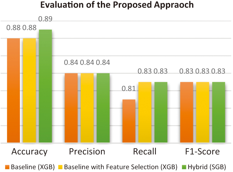
Figure 5 provides an overview of the evaluation of the proposed hybrid approach compared with the baseline models.
F.STATISTICAL TEST
Statistical significance was tested using the Wilcoxon signed-rank test (α = 0.05) to confirm whether improvements were non-random. Table XII presents the results of the Wilcoxon test.
Table XII. Results of the statistical test
| Clas. | p-Value | Significance |
|---|---|---|
| SVM | 0.008 | |
| KNN | 0.034 | |
| DT | 0.041 | |
| RF | 0.013 | |
| ANN | 0.056 | Not Significant |
| AB | 0.019 | |
| NB | 0.067 | Not Significant |
| QDA | 0.082 | Not Significant |
| JRip | 0.028 | |
| XGB | 0.011 | |
| GB | 0.017 | |
| DNN | 0.051 | |
| LR | 0.060 | Not Significant |
G.COMPARISON WITH EXISTING MODELS
The proposed method was compared with the existing hybrid models from the literature. As summarized in Table XIII, the proposed model achieved a superior accuracy of 87.1%, compared to 83.1% with K-means and SVM and 86.2% with PCA and RF. The results demonstrate the combined advantage of unsupervised grouping and selective feature reduction.
Table XIII. Hybrid-based diabetes prediction
| Ref. | SML | UML | CV | Accuracy |
|---|---|---|---|---|
| Proposed | XGB | K-means | √ | 87.1% |
| Edeh et al. [ | SVM | K-means | χ | 83.1% |
| Chang et al. [ | DT | PCA | χ | 86.24% |
V.RESULT ANALYSIS
A.IMPACT OF CLUSTERING INTEGRATION
As noted in the results, using clustering improved classification metrics across nearly all models. For instance, RF accuracy increased from 82.5% (non-clustered) to 87.1% (clustered). Similarly, XGB AUC improved from 0.86 to 0.90. These improvements are attributed to the enhanced feature separability obtained from the unsupervised stage, which reduced within-class overlap.
B.IMPACT OF FEATURE SELECTION
Applying MI-based feature selection reduced training time by approximately 35% on average without sacrificing performance. For example, the SVM model’s training time decreased from 2.8s to 1.9s, while accuracy remained nearly constant. The results confirm that removing redundant features effectively reduces computational complexity while retaining predictive power.
C.COMPARISON OF CLASSIFIERS
Ensemble models, specifically RF, XGB, and AB, consistently outperformed simpler models such as KNN and NB. Ensemble methods benefit from aggregating multiple weak learners, reducing overfitting and improving robustness to noise, which is critical in small, imbalanced datasets. The performance gain demonstrates the effectiveness of ensemble diversity when combined with cluster-based stratification.
D.EFFECT OF CLUSTER NUMBER
To confirm the selection of two clusters in the clustering process, Fig. 6 shows the accuracy of all classifiers with several cluster values. The two-cluster choice outperformed the others for all classifiers except the GB classifier.
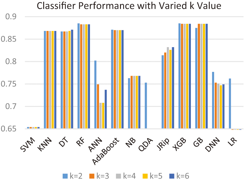 Fig. 6. Results of the proposed hybrid approach based on different numbers of clusters.
E.GENERALIZATION
The generalizability of this framework was assessed conceptually by comparing data characteristics of other medical datasets (e.g., Sylhet [32]). Since these datasets share small sample sizes and class imbalance, similar improvements in performance are expected. However, differences in feature distributions may require adaptive clustering strategies or autoencoder-based embedding.
VI.CONCLUSION
This study proposed a hybrid approach combining clustering with classification to enhance predictive model performance. The experimental results demonstrated that integrating clustering with supervised classification improved the accuracy, precision, recall, F1-score, and AUC metrics for most classifiers. The improvements were particularly notable for ensemble-based methods, such as RF, XGB, and GB, which consistently achieved the highest performance across various configurations. Besides, the study also highlighted limitations in simpler models, such as NB and QDA, which showed limited improvements despite the proposed approach. Overall, integrating clustering with classification significantly improves predictive performance, particularly for complex and ensemble-based classifiers. This demonstrates the potential of the proposed hybrid approach in real-world predictive modeling tasks. Future work could explore the impact of advanced clustering techniques, diverse feature selection methods, and optimal hyperparameter tuning to further enhance the proposed approach.