I.INTRODUCTION
Food security has long been recognized as one of the most critical global challenges, closely linked to the achievement of the United Nations Sustainable Development Goals (SDGs) [1]. Ensuring consistent access to affordable, safe, and nutritious food is fundamental to human development, yet many regions continue to experience volatility in both supply and distribution [2]. Increasing socioeconomic pressures, climate variability, and disruptions in global trade have further undermined food system stability, creating a demand for innovative approaches in prediction, monitoring, and management. Within this context, artificial intelligence (AI) and machine learning (ML) are increasingly applied to address such complexities through predictive analytics and data-driven decision support [3]. Indonesia, with its diverse agricultural base, illustrates both the opportunities and vulnerabilities of food systems management [4]. Aceh Province, in particular, represents a critical case due to its reliance on staple commodities such as rice, starchy foods, and fish [5].
Although local production remains central to food availability, recurring issues including price instability, inefficient distribution networks, and regional disparities in supply–demand balance continue to compromise system resilience [6]. Traditional statistical models often fall short in capturing these multidimensional and nonlinear interactions, thereby limiting their utility for long-term planning and effective policy design [7].
ML provides a promising alternative by integrating heterogeneous datasets and uncovering latent patterns in complex systems [8]. Predictive models such as regression, clustering, and classification enable the forecasting of commodity trends, identification of vulnerable regions, and classification of supply chain stability [9]. Recent studies have applied ML to agricultural forecasting, commodity price modeling, and supply chain analysis [10]. However, most approaches have remained methodologically fragmented, focusing on a single ML technique or lacking an integrated framework that can provide comprehensive and actionable insights for policy [11]. In the context of Aceh, fragmented applications of ML risk overlooking critical interdependencies between production, consumption, and population growth [12]. For example, regression models may predict future price trajectories but fail to identify stability levels within the supply chain, while clustering methods may group regions by vulnerability without providing forward-looking projections [13]. Addressing these limitations requires a more holistic framework that combines complementary ML methods to deliver both predictive accuracy and diagnostic clarity [14]. This study introduces an integrated ML framework that combines ridge regression for commodity price forecasting, K-means clustering for regional vulnerability detection, and random forest (RF) classification for supply chain stability analysis.
The contributions of this study are threefold. First, it proposes a multistage ML framework that unifies regression, clustering, and classification into a single system for smart food systems management. Second, it applies this framework to Aceh Province, a region characterized by unique food system dynamics but limited empirical research using advanced data-driven methods. Third, it provides empirical evidence of the policy relevance of ML-based decision support, demonstrating how predictive and diagnostic outputs can inform targeted interventions and strengthen food resilience.
Unlike prior studies that typically apply a single ML technique in isolation, this research advances a fully integrated framework that captures interdependencies across forecasting, clustering, and classification tasks. This holistic approach not only enhances methodological robustness but also ensures greater policy applicability, marking a clear novelty in the context of regional food systems optimization.
The remainder of this paper is structured as follows. Section II reviews related works on ML applications in food systems management and supply chain analysis. Section III outlines the methodology, including dataset description and the integrated ML framework. Section IV presents the results of regression forecasting, vulnerability clustering, and supply stability classification. Finally, Section V concludes the study and outlines directions for future research.
II.RELATED WORKS
In recent years, a growing body of research has examined the role of ML in addressing food security and optimizing supply chain management. Previous studies have primarily focused on global or national contexts, applying various predictive and classification models to assess production trends, price dynamics, and distribution vulnerabilities. These works demonstrate the potential of data-driven approaches to support decision-making in agriculture and food systems, particularly through techniques such as regression forecasting, clustering, and classification.
Despite these contributions, most existing studies remain concentrated on broader regions or specific commodities, leaving significant gaps at the subnational level. In particular, research addressing localized food system challenges in Aceh, Indonesia, is virtually absent. The unique socioeconomic characteristics, agricultural diversity, and regional vulnerabilities in Aceh necessitate a tailored approach that integrates both forecasting and classification within a unified framework.
Therefore, this study distinguishes itself by proposing an integrated ML framework specifically designed for the food system in Aceh. Unlike prior works that address food security at the global or national scale, this research combines regression forecasting, clustering optimization, and stability classification to generate actionable insights for regional policymakers. This contribution highlights the novelty of applying a comprehensive, localized analytical framework to support food system resilience in Aceh. Table I presents a comparative overview of previous works on ML applications in food security and supply chain management.
Table I. Comparative analysis of food security and supply chain research and differences with current study
| Reference | Methodology | Objectives | Techniques used | Key contributions |
|---|---|---|---|---|
| [ | Purposive and random sampling | Assess food security under COVID-19 and climate change | ANOVA | COVID-19 reduced yields and supply chain; climate change a major threat; recommended subsidies and adaptation |
| [ | Literature review; case studies (Canada and USA) | Examine COVID-19 impact on food security and GFSC; propose resilience framework | Analysis of open data and prior studies | Identified GFSC disruptions (labor, transport, production, and demand); proposed framework for smarter, resilient post-COVID-19 food supply chains |
| [ | Bibliometric analysis | Review evolution of agri-food supply chain research and identify trends | Topic mapping | Identified emerging topics (blockchain, IoT, resilience, and short food supply chains), hot topics (LCA, environmental impact, and food waste), and common SCM and SSCM practices |
| [ | PESTEL analysis; ANP and MAIRCA methods | Identify factors of blockchain in agri-food supply chains | PESTEL, Analytic Network Process (ANP), MAIRCA | Determined 12 critical success factors; highlighted top factors: “prevent food waste,” “increase food security,” “product lifecycle tracking”; linked blockchain adoption with circular economy and sustainability |
| [ | Comparative review | Explore urban farming’s impact on food supply in the USA and African cities | Literature review, policy, and case analysis | Highlighted role of urban farming in food security; identified success factors in USA |
| [ | Review and synthesis analysis | Examine benefits and challenges in food supply chains | Literature review, synthesis analysis | Enhances efficiency in food supply chains |
| [ | Review and conceptual framework | Examine blockchain and IoT integration in agri-food supply chains; propose architecture | Literature review, Agri-SCM-BIoT framework | Proposed blockchain + IoT architecture for transparency, traceability, security, privacy, and scalability |
| [ | Systematic literature review + single use-case analysis | Explore blockchain’s role in achieving operational excellence | CIMO logic, semi-structured interviews | Showed blockchain features (immutability, transparency, traceability, and smart contracts) enhance responsiveness, flexibility, efficiency, and collaboration in PFSC under COVID-19 |
| [ | Survey (n = 398, Thailand) | Identify drivers of (FDAs) | Partial least squares (PLS) | Practical implications for FDA retention strategies |
| [ | Time-series analysis | Predict food production for policymaking and food security planning | Machine learning: Adaptive Network-based Fuzzy Inference System (ANFIS) | ANFIS with Gbell membership functions provided lowest prediction error |
| Current study | Multistage machine learning framework | Optimize smart food systems management in Aceh through forecasting, vulnerability assessment, and supply chain monitoring | Ridge regression, K-means clustering with SAW centroid initialization, SVM (RBF and sigmoid), random forest | Integrated prediction, clustering, and classification for actionable insights; high forecasting accuracy optimized clustering (CH: 40.887; Silhouette: 0.288), and robust classification (SVM-RBF 94.59%, random forest 98.89%); supports evidence-based policy and resilience planning |
III.MATERIALS AND METHODS
This study applies a suite of ML approaches to advance smart food systems management in Aceh, Indonesia. The methodological framework encompasses three core components: commodity price forecasting, optimization of regional food vulnerability clustering, and classification of food supply chains.
A.PROPOSED METHOD
This study proposes a three-stage ML framework to enhance smart food systems management in Aceh, as illustrated in Fig. 1. The first stage focuses on commodity price forecasting using ridge regression, chosen for its ability to handle multicollinearity and provide stable predictions. Forecast accuracy is evaluated with mean squared error (MSE) and root mean squared error (RMSE) to ensure minimal prediction error.
 Fig. 1. Proposed method of machine learning approaches for smart food systems management in Aceh.
The second stage addresses regional food vulnerability clustering. K-means groups districts based on vulnerability profiles, while the integration of simple additive weighting (SAW) optimizes centroid initialization, enhancing cluster stability and interpretability. Clustering performance is measured using the Calinski–Harabasz (CH) index and Silhouette Score (SS) to ensure cohesion and separation.
The final stage involves classifying the food supply chain into distinct categories using support vector machine (SVM) and RF, representing margin-based and ensemble learning approaches. Model robustness and generalization are validated through 10-fold cross-validation to ensure statistically reliable results resistant to overfitting.
Algorithm selection at each stage is systematically guided by the Design of Experiments (DOE) framework [25], ensuring that choices are grounded in methodological reasoning rather than arbitrariness. The process relies on three key criteria: interpretability and policy relevance, computational efficiency relative to the dataset’s size and structure, and robustness against overfitting, verified through comprehensive cross-validation.
Accordingly, ridge regression is chosen for price forecasting due to its ability to handle multicollinearity while maintaining transparent coefficient interpretation. K-means is employed for clustering because of its simplicity and efficiency and is further refined via the SAW method to stabilize centroid initialization. For classification, SVM and RF are utilized to capture two distinct learning paradigms—margin-based and ensemble-based enabling a thorough comparative evaluation.
The DOE-guided framework ensures that algorithm selection is conducted in a structured, criteria-driven manner, promoting methodological rigor, transparency, and reproducibility over intuition or random choice.
B.FOOD COMMODITY PRICE FORECASTING USING A RIDGE REGRESSION MODEL
Price forecasting is conducted using ridge regression, a regularized linear regression technique designed to address multicollinearity and mitigate overfitting by introducing an L2 penalty term into the cost function, as formally expressed in Equation (1) [26]:
where represents the predicted commodity price, βj denotes the regression coefficients, and α is the regularization parameter optimized through cross-validation.The methodological procedure comprises the following steps:
1).DATA COLLECTION
The dataset employed in this study is obtained from the Aceh Food Agency (Dinas Pangan Aceh), which records the average annual retail prices of 12 strategic food commodities. The commodities include rice (premium and medium), dried soybeans, shallots, garlic, red chili peppers, beef, broiler chicken meat, chicken eggs, granulated sugar, packaged cooking oil, and wheat flour. The dataset spans from 2017 to 2024, as shown in Table II.
Table II. Annual average retail prices of strategic food commodities in Aceh (2017–2024)
| No | Commodity | 2017 | 2018 | 2019 | 2020 | 2021 | 2022 | 2023 | 2024 |
|---|---|---|---|---|---|---|---|---|---|
| 1 | Premium rice | 11.000 | 11.200 | 11.200 | 12.260 | 11.470 | 12.500 | 13.000 | 13.200 |
| 2 | Medium rice | 10.500 | 10.600 | 10.900 | 11.098 | 11.000 | 11.800 | 12.200 | 12.400 |
| 3 | Dried soybeans | 11.500 | 11.760 | 11.850 | 10.102 | 12.000 | 13.000 | 13.200 | 13.500 |
| 4 | Shallots | 35.000 | 33.400 | 26.300 | 38.062 | 30.715 | 34.000 | 36.500 | 37.000 |
| 5 | Garlic (bulb) | 24.300 | 25.850 | 30.000 | 31.600 | 26.206 | 28.000 | 29.000 | 30.200 |
| 6 | Curly red chili peppers | 35.375 | 28.500 | 38.000 | 32.371 | 34.739 | 36.000 | 38.000 | 40.000 |
| 7 | Pure beef | 125.000 | 132.900 | 140.000 | 140.879 | 147.500 | 150.000 | 153.000 | 155.000 |
| 8 | Broiler chicken meat | 26.000 | 27.000 | 27.500 | 29.735 | 27.406 | 30.000 | 31.200 | 32.000 |
| 9 | Broiler chicken eggs | 19.500 | 20.800 | 22.000 | 22.420 | 30.050 | 31.500 | 32.800 | 34.000 |
| 10 | Local granulated sugar | 12.500 | 13.000 | 13.000 | 14.832 | 14.000 | 15.000 | 15.500 | 16.000 |
| 11 | Packaged cooking oil (simple) | 10.000 | 10.000 | 10.500 | 11.484 | 16.178 | 17.500 | 18.000 | 18.500 |
| 12 | Bulk wheat Flour | 7.500 | 7.650 | 7.750 | 8.406 | 9.000 | 9.500 | 10.000 | 10.200 |
2).MODEL TRAINING
Ridge regression is applied, and cross-validation is performed to determine the optimal penalty parameter (α), minimizing predictive bias and variance.
4).MODEL EVALUATION
Predictive performance is assessed using standard statistical indicators, including MSE and RMSE, as expressed in Equations (2) and (3), respectively:
where n is the total number of observations. A lower MSE indicates that the predicted values are closer to the actual observed values, reflecting better model performance. MSE is particularly sensitive to large errors because deviations are squared, thus giving more weight to outliers.In this formula, denotes the observed value, is the predicted value, and is the number of observations. A lower RMSE indicates higher forecasting accuracy and makes interpretation easier compared to MSE.
C.REGIONAL FOOD VULNERABILITY CLUSTERING OPTIMIZATION
This stage assesses and optimizes regional food vulnerability in Aceh to identify districts requiring prioritized interventions. The analysis uses the Annual Food Supply and Demand Data Across Commodities in Aceh, with variables listed in Table III. Two clustering approaches are applied: standard K-means and SAW-K-means, which integrates SAW to improve centroid initialization, enhancing clustering stability and robustness.
Table III. Annual Food Supply and Demand Data Across Commodities in Aceh, Indonesia
| Variable | Description | Unit |
|---|---|---|
| Region | Name of the observed region/area | Region name |
| Year | Year of food data observation | Year |
| Population | Total population in the region for a specific year | People |
| Rice supply | Total rice availability in a specific year | Tons |
| Rice surplus | Difference between supply and demand of rice (positive = surplus, negative = deficit) | Tons |
| Starchy food supply | Availability of starchy foods (cassava, maize, sweet potato, etc.) | Tons |
| Starchy food demand | Total consumption demand for starchy foods | Tons |
| Starchy food surplus | Difference between supply and demand of starchy foods | Tons |
| Sugar supply | Total sugar availability | Tons |
| Oilseed surplus | Difference between supply and demand of oilseeds | Tons |
| Fruit supply | Availability of fruits | Tons |
| Fruit demand | Total fruit consumption demand | Tons |
| Fruit surplus | Difference between supply and demand of fruits | Tons |
| Vegetable supply | Availability of vegetables | Tons |
| Vegetable demand | Total vegetable consumption demand | Tons |
| Milk surplus | Difference between supply and demand of milk | Tons |
| Oil supply | Availability of edible oil (vegetable/animal-based) | Tons |
| Oil demand | Total oil consumption demand | Tons |
| Oil surplus | Difference between supply and demand of oil | Tons |
1).K-MEANS CLUSTERING
The K-means algorithm is applied through the following steps [27]:
- 1.Initialize centroidsRandomly select k initial centroids from the dataset to serve as starting points.
- 2.Assign districtsEach district i is assigned to the nearest centroid by minimizing the Euclidean distance, defined in Equation (4): where xi denotes the vector of vulnerability indicators for district i and μk is the centroid of cluster k.
- 3.Update centroidsRecompute each centroid μk as the mean of all points in cluster Ck.
- 4.Iterate until convergenceRepeat steps 2–3 until cluster assignments stabilize. The objective is to minimize the within-cluster sum of squares (WCSS), defined in Equation (5): where K is the number of clusters, is the set of districts in cluster k, and μk is the cluster centroid.
- 5.Evaluate cluster qualityThe clustering performance was quantitatively evaluated using the CH index and SS, defined in Equations (6) and (7): Tr(Bk) is the trace of the between-cluster dispersion matrix, Tr(Wk) is the trace of the within-cluster dispersion matrix, K is the number of clusters, and n is the total number of observations. Higher CH values indicate more distinct and well-separated clusters: a(i) is the average distance between observation i and other points in the same cluster, while b(i) is the minimum average distance to points in other clusters. The score ranges from −1 to 1, with higher values indicating more cohesive and well-separated clusters.
2).SAW-K-MEANS CLUSTERING
The SAW-K-means approach was implemented to enhance clustering stability and interpretability. By integrating SAW with K-means, cluster center initialization becomes more structured, reducing randomness, improving computational efficiency, and ensuring reliable clustering outcomes.
- 1.Compute Composite Vulnerability Scores.Each district i receives a composite score Si using SAW, defined in Equation (8) [28]: where wj is the weight of indicator, rij is the normalized value of indicator j for district i, and m is the total number of indicators. In this study, the weight wj is automatically assigned using an equal distribution method, yielding a value of 0.027778 for each criterion. The weighting process follows an equal-weight approach, where the total weight is evenly divided among all identified criteria. This method ensures that each criterion contributes equally to the overall assessment, thereby promoting fairness and minimizing potential bias toward any specific attribute in the final ranking outcome.
- 2.Initialize Centroids.Districts with the highest Si scores are selected as initial centroids to ensure highly vulnerable regions are represented from the outset.
- 3.Apply K-Means Algorithm.Follow the standard K-means procedure (assignment, centroid update, and iteration) using SAW-based centroids.
- 4.Evaluate Cluster Quality.Cluster quality was evaluated using CH index and SS
- 5.Identify Food Vulnerable Districts.Districts belonging to the cluster with the highest average Si were designated as Food Vulnerable areas.
D.FOOD SUPPLY CHAIN CLASSIFICATION
This research employs SVM and RF to classify food supply chain stability, as both algorithms are capable of handling high-dimensional datasets and modeling nonlinear dependencies. The models assigned districts to distinct classes based on supply chain characteristics using the Annual Food Supply and Demand Data Across Commodities in Aceh, with variables detailed in Table IV, offering actionable insights for policymakers to identify both stable and vulnerable regions.
Table IV. Variables for food supply chain classification
| Variable | Description |
|---|---|
| Commodity | Type of food commodity (e.g., rice, sugar, fish, vegetables, etc.) |
| District | Administrative region in Aceh where the data were collected |
| Year | Year of observation |
| Supply (tons) | Total food supply available in the district |
| Population | Total number of inhabitants in the district |
| Consumption requirement (tons) | Estimated food demand based on population size and dietary needs |
| Surplus (tons) | Difference between supply and consumption requirement |
| Status | Classification label indicating supply chain condition (e.g., surplus, deficit, or balanced) |
1).SUPPORT VECTOR MACHINE (SVM)
SVM is a supervised method designed to find the most effective hyperplane that distinguishes between classes [29]. For linearly separable data, the decision function is given in Equation (9):
where w represents the weight vector, x is the input feature vector, and b is the bias. The objective is to maximize the margin between support vectors. Mathematically, this objective can be expressed in Equation (10):For nonlinearly separable data, the kernel trick projects input features into a higher-dimensional space. Common kernels include the radial basis function (RBF), defined in Equation (11):
Here, γ controls the influence of individual samples. SVM was used to classify districts by mapping multidimensional food system features to an optimal decision boundary.
2).RANDOM FOREST (RF)
As an ensemble learning approach, RF strengthens classification performance through the integration of predictions from many individual decision trees [30]. Each decision tree is constructed using a bootstrap sample, with node divisions chosen from a randomly selected group of features. In this model, the concluding prediction is determined through a majority-vote mechanism across all decision trees, as represented in Equation (12):
In this equation, denotes the final predicted class label, where is determined based on the individual predictions generated by each decision tree within the ensemble. The mode function identifies the most frequently occurring class label among these predictions, thereby determining the overall output of the RF model through a majority voting mechanism. The splitting criterion in each decision tree is typically based on Gini Impurity, defined in Equation (13):
where pi is the proportion of samples belonging to class i and C is the number of classes.IV.RESULTS AND DISCUSSION
A.RESULTS OF FOOD COMMODITY PRICE PREDICTION USING A RIDGE REGRESSION MODEL
The first analysis stage forecasted food commodity prices using ridge regression, which mitigates multicollinearity and enhances model generalization through L2 regularization. Historical annual supply and demand data for Aceh are used to train the model and generate forecasts for 2025–2028. Performance was evaluated using MSE and RMSE. Table V and Fig. 2 present the forecasted prices for key commodities.
Table V. Forecasted food commodity prices in Aceh, Indonesia (IDR/kg), using ridge regression model
| Commodity | 2025 | 2026 | 2027 | 2028 |
|---|---|---|---|---|
| Premium rice | 15.277 | 16.223 | 17.170 | 18.117 |
| Medium rice | 14.332 | 15.207 | 16.082 | 16.957 |
| Dry soybeans | 15.391 | 16.337 | 17.283 | 18.228 |
| Red onion | 41.722 | 44.097 | 46.472 | 48.848 |
| Garlic bulb | 35.032 | 37.080 | 39.129 | 41.177 |
| Curly red chili | 44.885 | 47.635 | 50.384 | 53.134 |
| Fresh beef | 183.259 | 194.737 | 206.215 | 217.694 |
| Broiler chicken | 36.886 | 39.184 | 41.482 | 43.781 |
| Broiler eggs | 40.156 | 43.528 | 46.899 | 50.270 |
| Granulated sugar (local) | 18.577 | 19.790 | 21.002 | 22.215 |
| Packaged cooking oil (basic) | 22.098 | 24.070 | 26.041 | 28.012 |
| Wheat flour (bulk) | 11.904 | 12.748 | 13.591 | 14.435 |
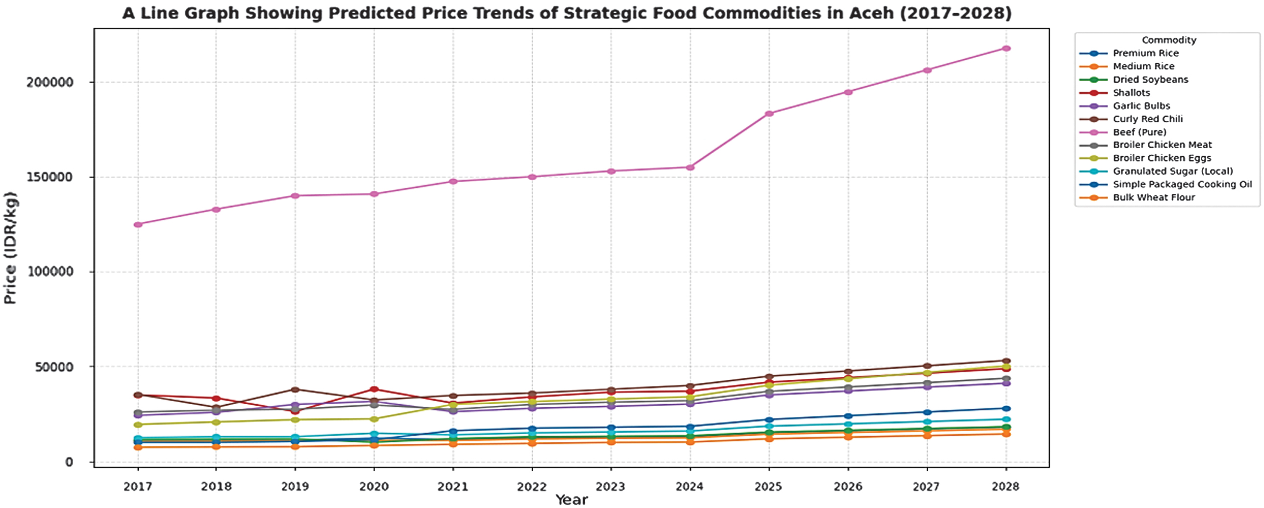 Fig. 2. Forecasted food commodity prices in Aceh, Indonesia (IDR/kg), using ridge regression model.
Forecasts indicate a general upward trend in Aceh’s food commodities from 2025 to 2028. Staple grains such as premium and medium rice and dry soybeans grow steadily, while high-value commodities like fresh beef and red chili rise sharply due to limited supply and market sensitivity. Perishable vegetables show significant increases, whereas processed goods grow moderately. Ridge regression highlights commodity vulnerability, with staples remaining resilient and high-demand items more exposed to shocks. Predictive accuracy, assessed using MSE and RMSE, provides insight into model performance, with Table VI comparing results across all commodities. Comparative error analysis of ridge regression reveals substantial variations across commodities. Beef shows the highest errors due to supply shocks and seasonal demand, while shallots, red chili, and garlic also exhibit elevated errors from perishability and climate sensitivity. Staples like wheat flour, medium rice, and cooking oil have the lowest errors, reflecting stable markets, with sugar and dried soybeans in the mid-range. MSE highlights extreme deviations, while RMSE provides a unit-consistent measure of forecast accuracy. Fig. 3 and 4 visualize these results.
Table VI. Comparative evaluation of predicted food commodity prices (2025–2028)
| No | Commodity | MSE | RMSE |
|---|---|---|---|
| 1 | Beef (pure) | 394,006,100 | 19,849.586 |
| 2 | Shallots | 31,715,200 | 5,631.625 |
| 3 | Curly red chili | 29,310,450 | 5,413.912 |
| 4 | Garlic bulbs | 18,905,290 | 4,348.021 |
| 5 | Broiler chicken meat | 16,452,640 | 4,056.185 |
| 6 | Broiler chicken eggs | 9,751,155 | 3,122.684 |
| 7 | Granulated sugar (local) | 3,783,863 | 1,945.215 |
| 8 | Dried soybeans | 3,224,823 | 1,795.779 |
| 9 | Premium rice | 2,842,324 | 1,685.919 |
| 10 | Simple packaged cooking oil | 2,756,257 | 1,660.198 |
| 11 | Medium rice | 2,539,593 | 1,593.610 |
| 12 | Bulk wheat flour | 1,263,658 | 1,124.126 |
| 394,006,100 | 19,849.586 |
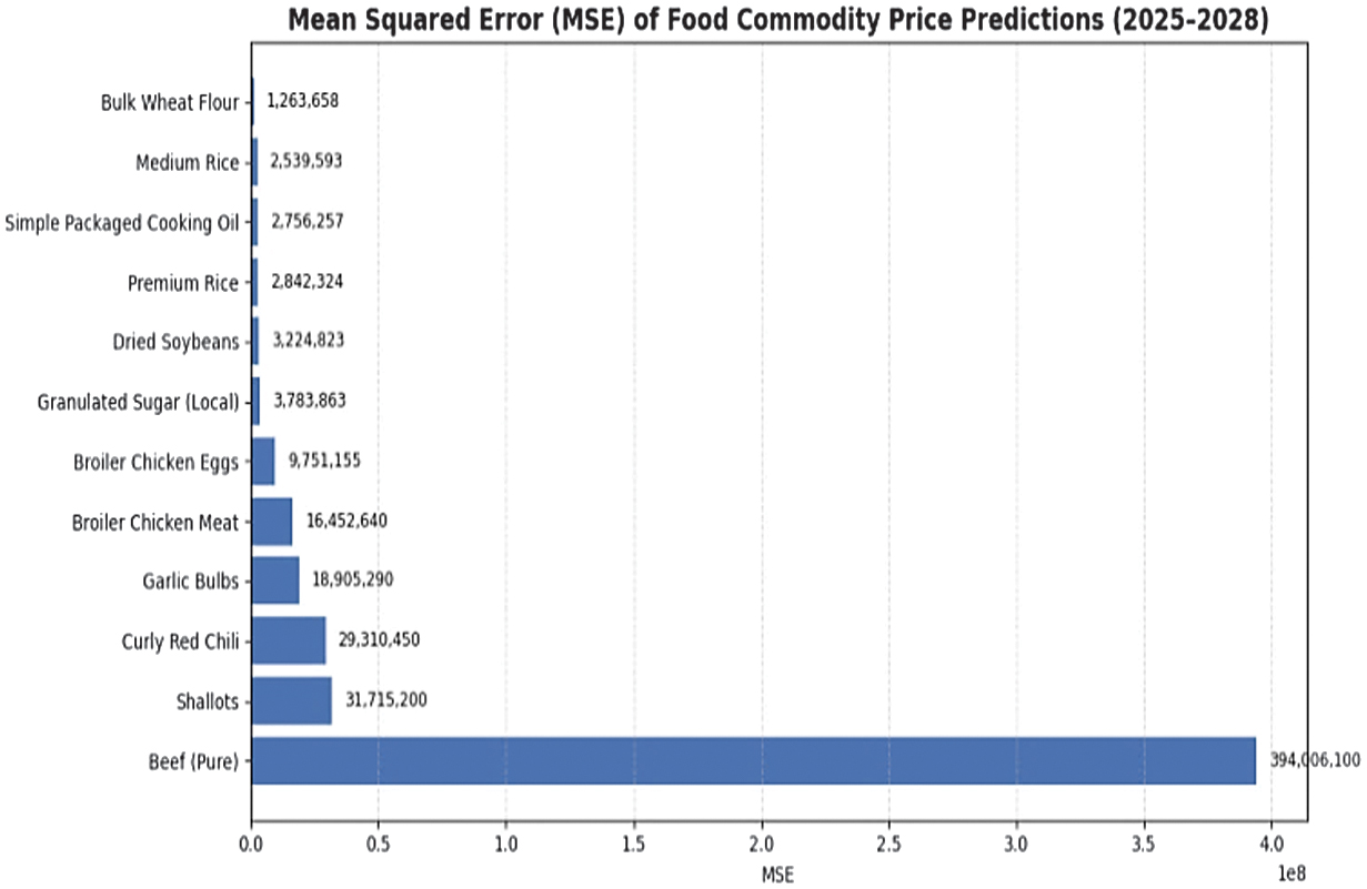 Fig. 3. Mean squared error (MSE) of ridge regression predicted food commodity prices (2025–2028) in Aceh.
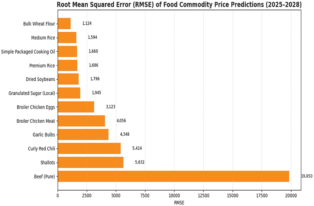 Fig. 4. Root mean squared error (RMSE) of ridge regression predicted food commodity prices (2025–2028) in Aceh.
Table VII displays the evaluation results of the ridge regression model across multiple K-fold cross-validation configurations. The primary objective of this experiment is to identify the optimal number of folds (K) that produces the most reliable and accurate model performance. Each configuration is evaluated using two principal performance metrics: MSE and RMSE, which quantify, respectively, the average magnitude of prediction errors and the extent of their variability. The cross-validation results show that the ridge regression model performs consistently across different fold settings. The lowest MSE occurs at K = 6, indicating a balanced bias–variance trade-off, while the lowest RMSE is achieved at K = 8, reflecting greater predictive stability. Therefore, K = 8 is considered the optimal configuration for subsequent evaluation and forecasting, as it minimizes prediction error and ensures robust validation.
Table VII. Evaluation results of ridge regression with various K-fold cross-validation values
| No | Number of folds (K) | MSE | RMSE | Remark |
|---|---|---|---|---|
| 1 | 5 | 83,835,322.18 | 5,229.04 | – |
| 2 | 6 | 77,351,844.18 | 4,834.10 | Lowest MSE |
| 3 | 7 | 81,319,392.70 | 5,010.14 | – |
| 4 | 8 | 79,878,235.49 | 4,727.36 | Lowest RMSE |
B.RESULTS OF REGIONAL FOOD VULNERABILITY CLUSTERING OPTIMIZATION
The second stage of this study examines regional food vulnerability clustering to identify districts in Aceh that require prioritized interventions. Two approaches are implemented: the standard K-means clustering and the enhanced SAW-K-means clustering. Both methods aimed to classify districts into distinct vulnerability groups based on their food supply–demand balance across multiple commodities. The integration of the SAW method into the initialization process was designed to reduce randomness in centroid selection, thereby enhancing clustering stability and interpretability.
Clustering identifies three categories: Food Secure, Food Vulnerable, and Food Insecure. Food Secure districts have stable surpluses, reflecting a resilient supply chain. Food Vulnerable districts experience fluctuating supply–demand balances, indicating potential exposure to shocks. Food Insecure districts faced persistent deficits, highlighting structural weaknesses in availability and distribution. SAW-K-means produces a more balanced and interpretable distribution than standard K-means, with the Food Insecure cluster aligning closely with official vulnerability indicators.
1).STANDARD K-MEANS CLUSTERING RESULTS
Standard K-means is applied to classify food vulnerability across Aceh districts into three categories: Food Secure, Food Vulnerable, and Food Insecure, with results shown in Table VIII. Coastal urban districts such as Banda Aceh, Sabang, and Lhokseumawe were Food Secure, reflecting stable food access and infrastructure. Remote inland districts, including Gayo Lues, Aceh Tenggara, Simeulue, and Bener Meriah, were Food Insecure due to geographic isolation and limited productivity. Most other districts, such as Pidie, Aceh Utara, and Aceh Timur, were Food Vulnerable, indicating susceptibility to supply–demand fluctuations. Cluster distribution from 2017 to 2024 is shown in Fig. 5, with a corresponding heatmap in Fig. 6.
Table VIII. Standard K-means clustering results for food vulnerability in Aceh Province, Indonesia
| Cluster category | Districts |
|---|---|
| Banda Aceh, Sabang, Lhokseumawe, Langsa, Subulussalam | |
| Aceh Besar, Pidie, Bireuen, Aceh Utara, Aceh Timur, Aceh Tamiang, Aceh Jaya, Aceh Barat Daya, Nagan Raya, Aceh Selatan | |
| Gayo Lues, Aceh Tenggara, Aceh Singkil, Simeulue, Bener Meriah, Aceh Tengah |
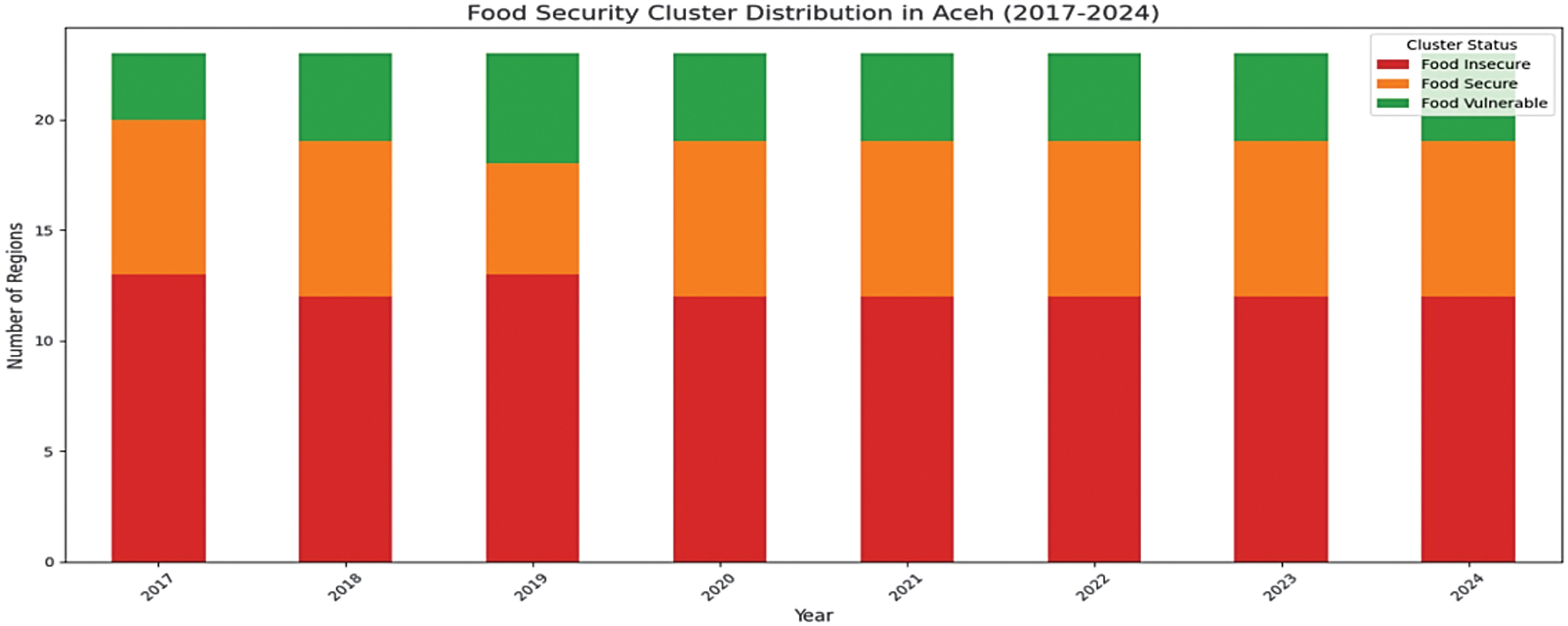 Fig. 5. Food security cluster distribution in Aceh, Indonesia (2017–2024).
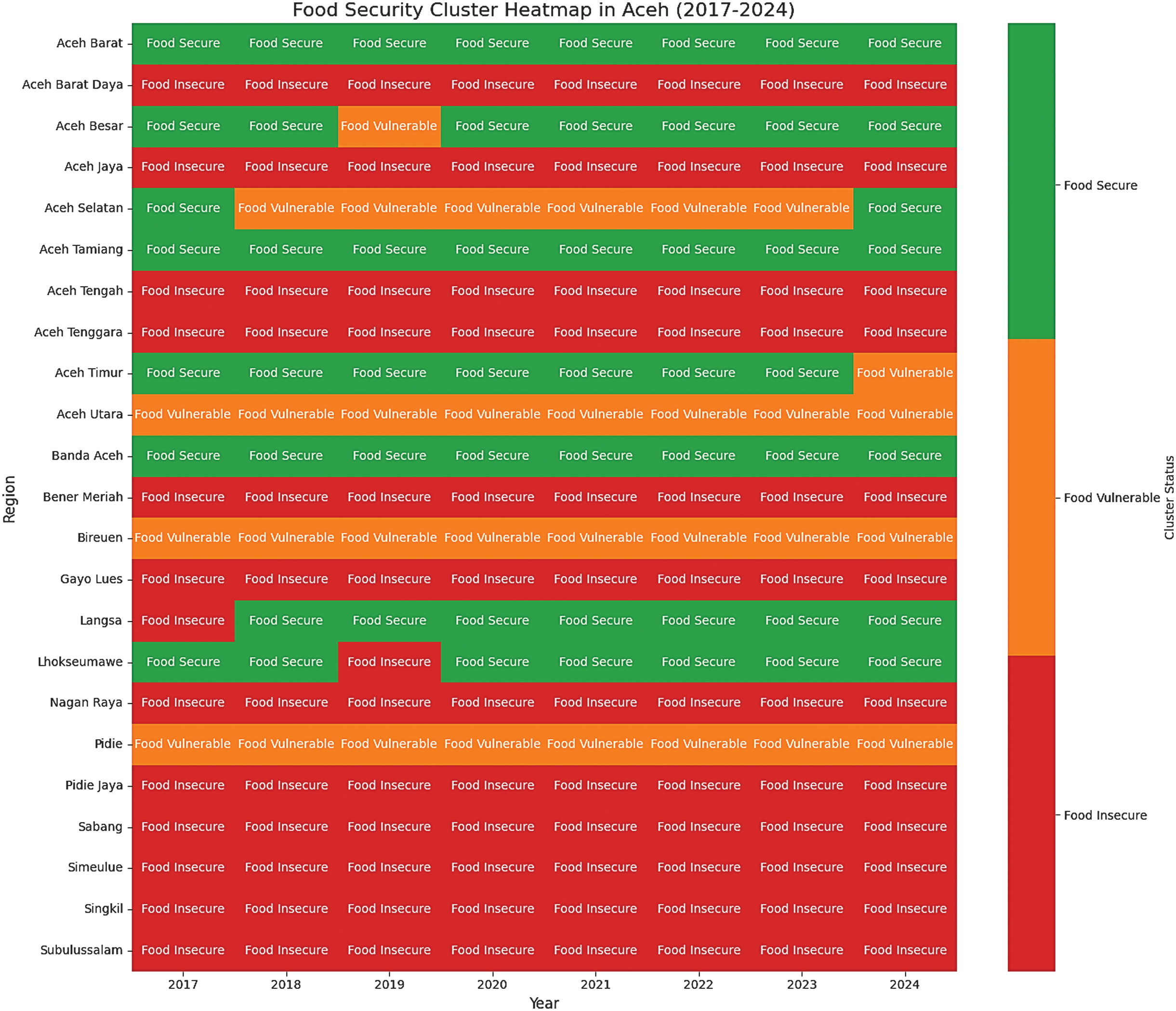 Fig. 6. Food security heatmap cluster distribution in Aceh, Indonesia (2017–2024).
To assess the performance and stability of the K-means algorithm, ten runs with different initial centroid selections were conducted. Convergence speed was measured by iteration count, while clustering quality was evaluated using the CH index and the SS. Results show that the CH index remained high (≈45.5) and the SS stable at 0.30, reflecting consistent cluster separability with moderate cohesion. Test 4 achieved the best outcome (CH = 45.75, 6 iterations), while Test 6 performed worst (CH = 35.35, Silhouette = 0.29). Overall, K-means proved robust, though centroid initialization influenced efficiency and cluster quality as shown in Table IX.
Table IX. Performance evaluation of K-means iterations with different initial centroids
| Test no. | Initial centroids (data index) | Number of iterations | Calinski–Harabasz index | Silhouette Score |
|---|---|---|---|---|
| 1 | 42, 142, 183 | 11 | 45.54 | 0.30 |
| 2 | 4, 124, 43 | 8 | 45.54 | 0.30 |
| 3 | 91, 178, 48 | 9 | 45.38 | 0.30 |
| 4 | 146, 169, 13 | 6 | 45.75 | 0.30 |
| 5 | 61, 123, 84 | 9 | 45.69 | 0.30 |
| 6 | 61, 155, 32 | 6 | 35.35 | 0.29 |
| 7 | 123, 137, 13 | 7 | 45.67 | 0.30 |
| 8 | 70, 74, 22 | 14 | 45.64 | 0.30 |
| 9 | 91, 62, 28 | 11 | 45.38 | 0.30 |
| 10 | 79, 80, 47 | 6 | 45.67 | 0.30 |
2).SAW K-MEANS CLUSTERING RESULTS
The SAW-K-means method applies SAW to calculate feature weights, enabling more systematic centroid initialization and improving cluster distinction. This refinement addresses the key limitations of conventional K-means, namely its sensitivity to random centroid selection and the assumption of equal feature importance. The results are summarized in Table X.
Table X. SAW scores and rankings for the regions
| No. | SAW score | Ranking |
|---|---|---|
| 153 | 15.3446 | 1 |
| 155 | 14.1372 | 2 |
| 128 | 8.6737 | 3 |
| 154 | 8.1976 | 4 |
| 109 | 7.4991 | 5 |
| 88 | 7.3506 | 6 |
| 125 | 7.1899 | 7 |
| 168 | 6.8346 | 8 |
| 166 | 6.7663 | 9 |
| 167 | 6.7093 | 10 |
Table X presents the top 10 results from a dataset of 184 regions ranked using the SAW method. In the SAW-K-means hybrid framework, centroid initialization was guided by SAW rankings, with one centroid each selected from the highest, middle, and lowest scores across 10 test iterations. Clustering performance was subsequently assessed using CH index and SS, demonstrating improved stability and quality through the integration of prior ranking information as shown in Table XI.
Table XI. SAW-K-means performance evaluation
| Test no. | Initial centroids (data index) | Iterations | CH score | Silhouette Score |
|---|---|---|---|---|
| 1 | 153, 116, 12 | 8 | 35.35 | 0.29 |
| 2 | 155, 102, 24 | 8 | 35.17 | 0.29 |
| 3 | 128, 103, 146 | 9 | 45.37 | 0.3 |
| 4 | 154, 115, 80 | 4 | 33.72 | 0.3 |
| 5 | 109, 75, 35 | 8 | 45.21 | 0.3 |
| 6 | 88, 101, 38 | 8 | 45.69 | 0.3 |
| 7 | 125, 6, 138 | 11 | 45.09 | 0.3 |
| 8 | 168, 20, 98 | 7 | 31.85 | 0.2 |
| 9 | 166, 53, 4 | 7 | 45.72 | 0.3 |
| 10 | 167, 36, 74 | 5 | 45.7 | 0.3 |
Table XI presents the clustering performance of the SAW-K-means hybrid method across 10 iterations. Using SAW for centroid initialization enhances stability, with CH indices ranging from 31.85 to 45.72 and SSs mostly around 0.3. Iterations 3, 6, 9, and 10 achieve higher CH scores above 45, indicating clearer cluster separation, while iteration 8 records the weakest performance with the lowest CH (31.85) and Silhouette (0.2). These results confirm that SAW-based centroid selection improves consistency and reliability, with iteration counts (4–11) reflecting adaptive convergence. A comparison of average results with standard K-means is shown in Table XII and Fig. 7.
Table XII. Comparison of average performance metrics between standard K-means and SAW-enhanced K-means
| Method | Average iterations | Average CH score | Average silhouette |
|---|---|---|---|
| SAW + K-means | 7.5 | 40.887 | 0.288 |
| K-means | 8.7 | 44.561 | 0.299 |
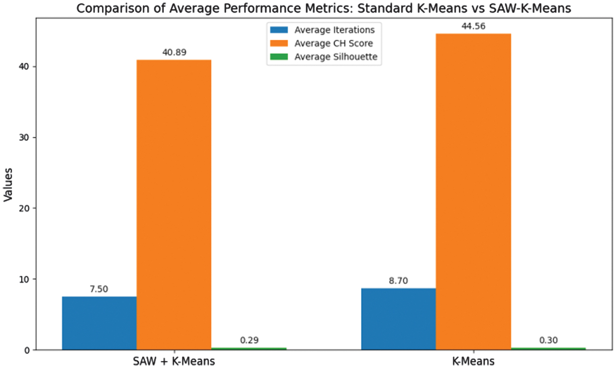 Fig. 7. Comparison of average performance metrics: standard K-means vs. SAW-K-means.
The comparison between standard K-means and SAW-K-means shows that SAW-based centroid initialization improves convergence speed (7.5 vs. 8.7 iterations). While standard K-means achieves slightly higher CH (44.561 vs. 40.887) and SSs (0.299 vs. 0.288), the differences are marginal, indicating comparable clustering quality overall.
C.RESULTS OF FOOD SUPPLY CHAIN CLASSIFICATION
In this stage, the stability of the food supply chain across districts in Aceh is assessed using supervised learning algorithms, specifically SVM and RF. The classification models were trained to categorize regions into predefined supply chain stability classes, leveraging features such as commodity supply, population demand, and surplus levels.
1).SVM RESULTS
SVM is applied to classify the stability of food supply chains by testing two kernel functions, namely RBF and sigmoid. Both kernels are selected to capture nonlinear relationships within the dataset, while variations of the penalty parameter C and kernel coefficient γ are analyzed to optimize performance. The results of SVM classification with the RBF kernel are summarized in Table XIII and Fig. 8.
Table XIII. Classification accuracy of SVM with RBF kernel for different values of C and γ
| C | γ (Gamma) | Mean accuracy (%) |
|---|---|---|
| 100 | 0.01 | 75.92 |
| 100 | 0.1 | 83.70 |
| 100 | 1.0 | 90.28 |
| 100 | 5.0 | 91.59 |
| 100 | 15.0 | 92.61 |
| 100 | 50.0 | 93.51 |
| 200 | 0.01 | 77.99 |
| 200 | 0.1 | 84.45 |
| 200 | 1.0 | 91.53 |
| 200 | 5.0 | 92.37 |
| 200 | 15.0 | 93.48 |
| 200 | 50.0 | 94.59 |
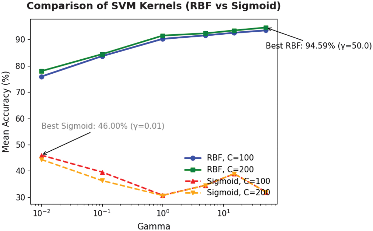 Fig. 8. Comparison of classification accuracy of SVM with RBF and sigmoid kernels for different values of C and γ.
SVM with RBF kernel showed strong sensitivity to C and γ, with accuracies below 85% at low γ (0.01–0.1) and improving above 90% for C = 100–200. The best accuracy of 94.59% occurred at C = 200 and γ = 50. SVM with sigmoid kernel was also evaluated across C and γ to assess its handling of nonlinear separability. In Table XIV, the SVM with a sigmoid kernel was evaluated across varying C and γ values to assess its capability in modeling nonlinear separability within the dataset.
Table XIV. Classification accuracy of SVM with sigmoid kernel for different values of C and γ
| C | γ (Gamma) | Mean accuracy (%) |
|---|---|---|
| 100 | 0.01 | 46.00 |
| 100 | 0.1 | 39.59 |
| 100 | 1.0 | 30.74 |
| 100 | 5.0 | 34.50 |
| 100 | 15.0 | 38.92 |
| 100 | 50.0 | 31.99 |
| 200 | 0.01 | 44.37 |
| 200 | 0.1 | 36.33 |
| 200 | 1.0 | 30.65 |
| 200 | 5.0 | 34.50 |
| 200 | 15.0 | 38.95 |
| 200 | 50.0 | 31.99 |
The sigmoid kernel performed poorly, reaching a maximum accuracy of only 46% (C = 100, γ = 0.01), with most results fluctuating between 30 and 40%, indicating instability and underfitting. In contrast, the RBF kernel consistently delivered superior performance, attaining 94.59% at optimal settings, thereby demonstrating its effectiveness in modeling food supply chain stability.
2).RF RESULT
The classification performance of the RF model across the three stability classes is presented in Table XV. This report provides a detailed overview of the precision, recall, and F1-scores, highlighting the model’s consistency in classifying Adequate, Deficit, and Surplus conditions.
Table XV. Classification report of random forest classifier
| Metric/class | Adequate | Deficit | Surplus | Accuracy/fold accuracies |
|---|---|---|---|---|
| Precision | 0.9948 | 0.9886 | 0.9835 | Fold 1: 99.13% |
| Recall | 0.9948 | 0.9808 | 0.9913 | Fold 2: 97.97% |
| F1-score | 0.9948 | 0.9847 | 0.9874 | Fold 3: 98.55% |
| Support | 1145 | 1145 | 1145 | Fold 4: 99.13% |
| Macro avg | 0.9890 | 0.9889 | 0.9889 | Fold 5: 98.84% |
| Weighted avg | 0.9890 | 0.9889 | 0.9889 | Fold 6: 99.71% |
| Overall accuracy | 0.9889 | Fold 7: 99.42% | ||
| Fold 8: 97.38% | ||||
| Fold 9: 100.00% | ||||
| Fold 10: 98.83% | ||||
| Mean accuracy: 98.89% | ||||
| Std. dev: 0.75% |
RF consistently classified food supply chain stability with high performance, achieving F1-scores of 0.985–0.995, a mean 10-fold accuracy of 98.89%, and low variability (0.75%). The RF model is configured with the hyperparameter n_estimators = 100, which specifies the number of decision trees in the ensemble. This value strikes an effective balance between model accuracy and computational efficiency, as adding more trees beyond this point typically yields diminishing performance improvements. The parameter random_state = 42 is applied to ensure the reproducibility of results across different runs. Other hyperparameters, including max_depth, min_samples_split, and min_samples_leaf, are retained at their default settings, allowing the model to adjust dynamically to the dataset’s characteristics. The chosen configuration is evaluated using 10-fold stratified cross-validation, which confirms stable and reliable model performance without the need for extensive hyperparameter optimization.
3).COMPARISON OF SVM AND RF CLASSIFICATION PERFORMANCE
As shown in Fig. 9, RF outperformed SVM, achieving 98.89% mean accuracy, low variability (std. dev = 0.75%), and high F1-scores (0.985–0.995), making it the more robust and reliable model.
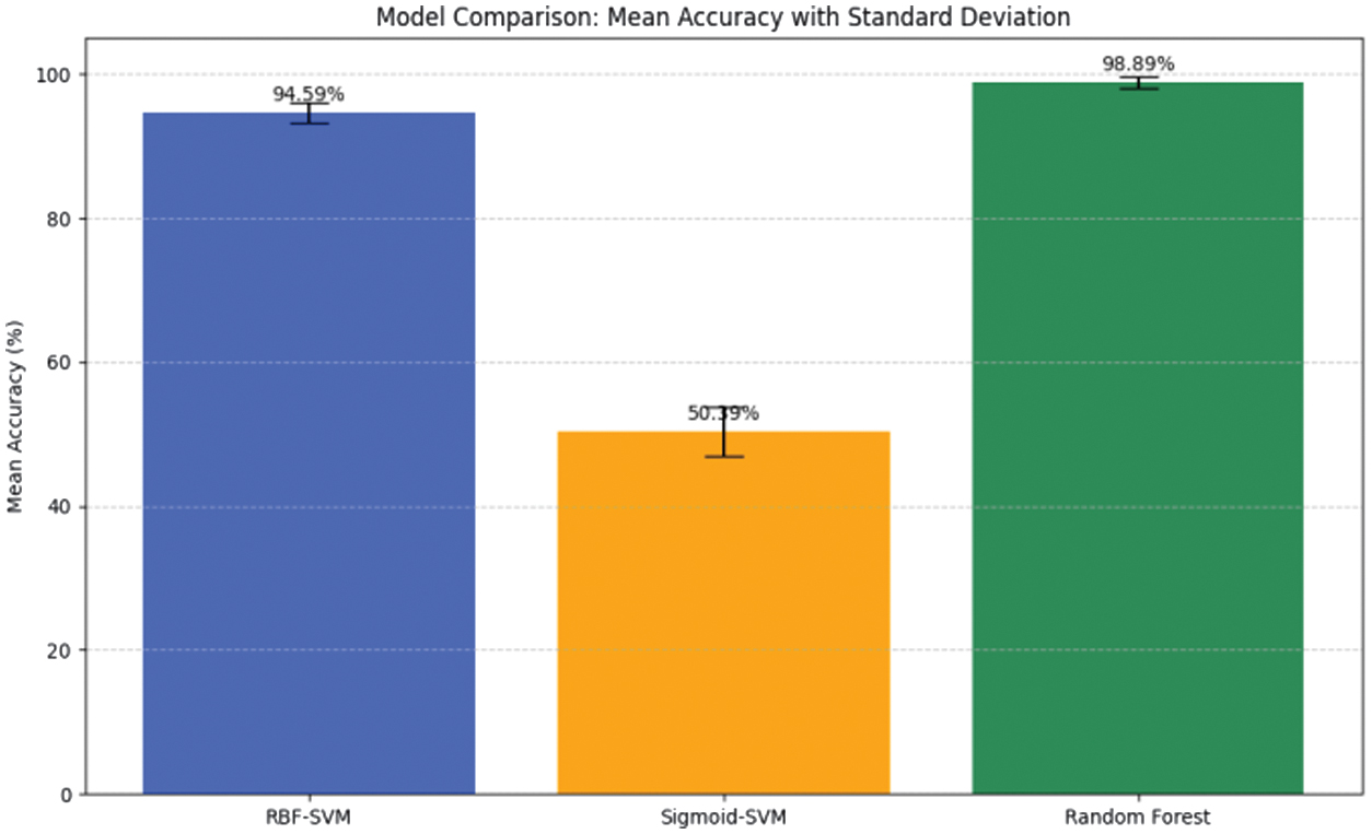 Fig. 9. Comparative accuracy of SVM and random forest models in classifying regional food supply chain stability.
Beyond the comparison between SVM and RF in this study, other ensemble methods, such as LightGBM, modified KNN, and decision trees, can be explored in future work. While boosting-based models often achieve slightly higher accuracy, they remain more sensitive to hyperparameter tuning and demand greater computational resources. In contrast, RF offers a balanced trade-off between accuracy, stability, and interpretability, making it particularly well suited for policy-oriented analyses. Consequently, its selection in this framework is methodologically justified, with boosting-based ensembles proposed for subsequent evaluation.
V.CONCLUSION
This study developed a multistage ML framework to analyze food commodity price dynamics and supply chain stability in Aceh, Indonesia. By combining ridge regression, SAW-K-means clustering, and RF classification, the framework provided a comprehensive approach to forecasting prices, identifying regional vulnerabilities, and classifying supply chain stability. Ridge regression effectively forecasted commodity prices for 2025–2028, addressed multicollinearity challenges, and captured trends across both staple and high-value commodities. While volatility was more evident in perishable and high-demand products, staple commodities demonstrated greater predictability.
In the clustering stage, standard K-means grouped districts into Food Secure, Food Vulnerable, and Food Insecure categories; however, its sensitivity to centroid initialization limited clustering stability. The SAW-K-means hybrid addressed this limitation by producing more balanced clusters that aligned better with official food vulnerability indicators, thereby improving interpretability for policymakers. For the classification stage, the SVM with an RBF kernel achieved 94.59% accuracy but required careful hyperparameter tuning, whereas the sigmoid kernel underperformed. The RF model achieved the highest performance, with a mean accuracy of 98.89%, low variance across folds (std. dev = 0.75%), and F1-scores between 0.985 and 0.995, confirming its robustness as a reliable classifier for food supply chain monitoring.
Overall, the framework underscored the value of integrating regression, clustering, and ensemble-based classification for the management of regional food systems. It provided policymakers with a decision-support capability to anticipate price fluctuations, prioritize interventions, and design targeted food security strategies. However, the study remained limited by its dataset, which covered only Aceh Province and therefore restricted the generalizability of the findings to broader contexts. Although the framework was developed and validated using food system data from Aceh Province, its modular structure enabled adaptation to other datasets and geographical regions. The ridge regression component could be retrained with local commodity price data to forecast market dynamics in new locations. The SAW-K-means clustering procedure could be recalibrated by redefining vulnerability indicators based on regional priorities. In the classification stage, both SVM and RF models could be applied to different commodity types or supply chain environments by relabeling classes and re-optimizing hyperparameters through cross-validation. The proposed framework was thus transferable and adaptive, allowing implementation across provinces, countries, or datasets with similar structural characteristics. Future studies should extend the framework to multiregional datasets, explore hybrid ensemble classifiers, and incorporate more advanced temporal forecasting techniques to improve scalability and policy relevance.