I.INTRODUCTION
In the concept of sustainable digital village development [1], agriculture signifies an economic sector that requires attention. A process carried out in agriculture involves detecting diseases [2]. Continuous and prompt recognition of agricultural goods is necessary. Traditionally, farmers must set aside time for oversight tasks. Farmers often face challenges that include the considerable time required. Not all farmers have knowledge about pests and plant diseases, and the large land area makes this process even more difficult.
Identifying plant diseases can be done through various methods, including laboratory testing [3] and by directly observing the plants [3]. To meet execution needs, direct observation provides the solution. Plant diseases can be directly identified through multiple means, such as observing leaves, stems, roots, and other parts of the plant. Leaves have been widely employed in the detection process for identifying pests and diseases [4–10], evaluating nutrient levels in plants [11–15], measuring leaf area [16], examining leaf structure [17], assessing freshness [18,19], and determining soil nutrients in plants [20]. A variety of plants has been studied using data obtained from leaves, including muskmelon [21], corn [4,22], potato [5,23], tomato [6,24,25], plum [8], melon [20,26–31], apple [9], bitter gourd [18], bottle gourd [18], cauliflower [18], eggplant [18], cucumber [18], watermelon [10], safflower [17], and paddy [11,20,32].
Research has also been carried out on detecting diseases in melon plants through their leaves [19,26–31]. Many research efforts have focused on ascertaining the health conditions of plants [19,31], recognizing diseases impacting melon plants [26–28,30], or evaluating the intensity of diseases in melon plants [29]. The methods used were varied, including Convolutional Neural Networks (CNNs) [19,29], Artificial Neural Networks (ANNs) [26], Decision Trees (DTs) [31], Gradient Boosting (GB) [30], Random Forest (RF) [30], XGBoost (XGB) [30], Logistic Regression (LR) [31], Support Vector Machine (SVM) [29], Naïve Bayes (NB) [31], ResNet50 (50-Layer Residual Network) [29], YOLOv5 [16,26], YOLOv8 [26], and YOLOv9 [26]. Different techniques were used to identify diseases via the leaves of melon plants. The YOLO (You Only Look Once) series provided a detection framework that necessitates the leaf image to contain a class label along with a bounding box showing the region to be recognized.
This research seeks to explore disease identification via melon plant leaves by assessing the effectiveness of various methods and contrasting the accuracies of the resulting models, employing techniques such as machine learning, deep learning, and YOLO. The document is structured as follows: Section I provides the introduction and context of the study, Section II reviews the literature that underpins this research, Section III outlines the research methodology employed in this study, Section IV analyses the results of the study, and Section V presents the conclusions.
II.LITERATURE REVIEW
Different techniques can be employed to identify the onset of diseases in melon plants using the leaves of melon plants as input. There are three categories of methods for this purpose: the supervised machine learning methods [26,29–31], the deep learning methods [19,29], and the YOLO methods [16,26]. Every model accommodates the distinct characteristics. These traits set apart the modeling process, including the necessity for preprocessing, feature extraction, augmentation, labeling, bounding box configuration, and various other procedures [26,29–31].
Assorted options can be utilized in preprocessing stages, including manual methods like background removal, cropping, contrast enhancement, normalization, among others [26,29–31]. Removing backgrounds is particularly crucial since images captured from fields or experimental locations may have several types of backgrounds. This method may prevent excessive learning about the backgrounds.
Leaf images can yield a variety of extractable features. These factors consist of the ratio of colors in the leaf, the makeup of segments in the leaf, the leaf’s color moment, edges, leaf veins, color patches, powdery marks, necrosis, signatures of disease types, and more [26,29–31]. The extent of different extractable features has been demonstrated to notably influence modeling outcomes [29].
Manual feature extraction leads to a restricted quantity of features being extracted. For greater automatic feature extraction, a pretrained model like ResNet50 may be utilized [29]. This method allows for the extraction of as many as 2048 features from a single image. The result of raising the count of features extracted is that the model development could require more time [29].
In machine learning, several traditional techniques may be included in the study such as ANN [26], DTs [31], GB [30], LR [31], NB [31], SVMs [29], and XGB [30]. Every technique has its unique procedures for creating a classification model. Several parameters must be configured, and the values can be modified to align with the characteristics of the input data.
In contrast, CNN could handle the modeling by directly taking in images. The images can be either the original form or the processed form [19,29]. CNN might also be combined with models that have been pretrained, such as ResNet50 [29]. Nonetheless, incorporating ANN within CNN was inevitable.
YOLO modeling [16,26] offers diversity in classification outcomes. In addition to the class category as the modeling results, it also offers the position of the object to be recognized. In certain situations, the processes of labeling and creating bounding boxes still need special attention. The process of setting labels and bounding boxes with a pretrained model remains unworkable in certain situations. Different versions of YOLO exist for modeling, such as YOLOv5 [16,26], YOLOv8 [26], and YOLOv9 [26].
When conducting modeling, several factors must be considered. They encompass the evaluation of whether the training data is balanced or not. If the data show imbalance, it is necessary to adjust the training data, since the quantity of data will influence both the training and testing processes [33,34]. Modeling techniques also come with a range of supportive parameters that need to be considered. The values of the parameters also affect the accuracy of predictions made by the models in question. Adjusting the parameters is essential to verify that the selected parameters represent the optimal selection for the modeled data compared to other potential values [35].
To assess the classification methods, several performance metrics can be utilized. They encompass accuracy, mean precision, mean recall, mean F1-score, and more [16,26,29–31,34,35]. Precision for each class could also be examined to gain insight into the modeling outcomes. For object detection, mean Average Precision (mAP) may be utilized [16,26]. The latter is utilized to assess the accuracy of the identified locations of the objects of interest.
III.RESEARCH METHOD
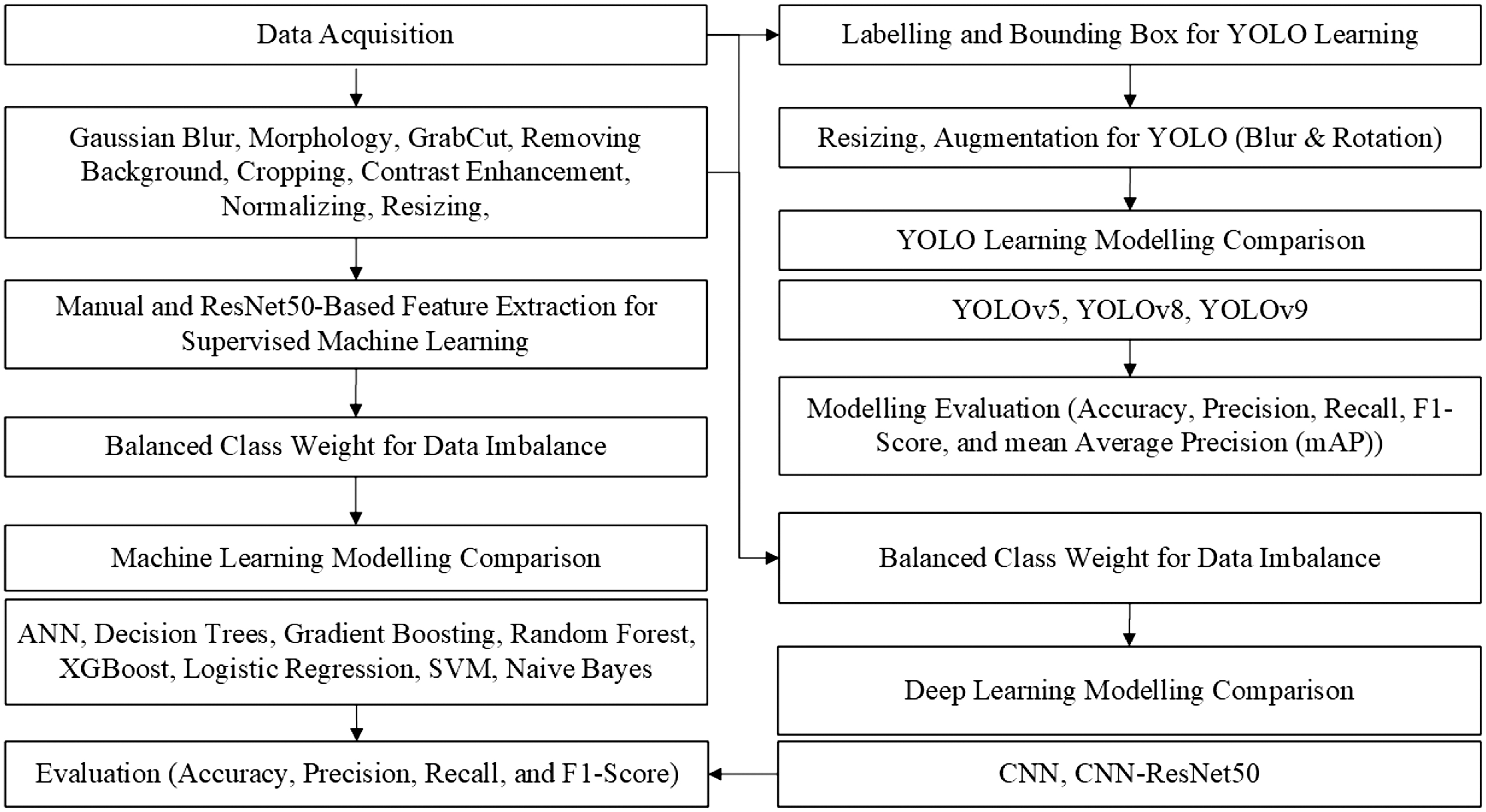
As shown in Fig. 1, the research procedures are conducted as follows:
- 1.Data collection is conducted to obtain melon leaf image data for four disease categories: Anthracnose (1), Leafminer (2), Powdery (3), and Scab (4), plus one Healthy category (0).
- 2.Data preprocessing takes place before modeling. In machine learning modeling, the data preprocessing steps include Gaussian blur, morphology, GrabCut, background removal, cropping, contrast enhancement, normalization, and resizing. The same preprocessing is applied for deep learning modeling. Still, in deep learning, in addition to utilizing preprocessed images, direct modeling from the original images is also conducted. In YOLO modeling, resizing and transformations like blur and rotation are applied.
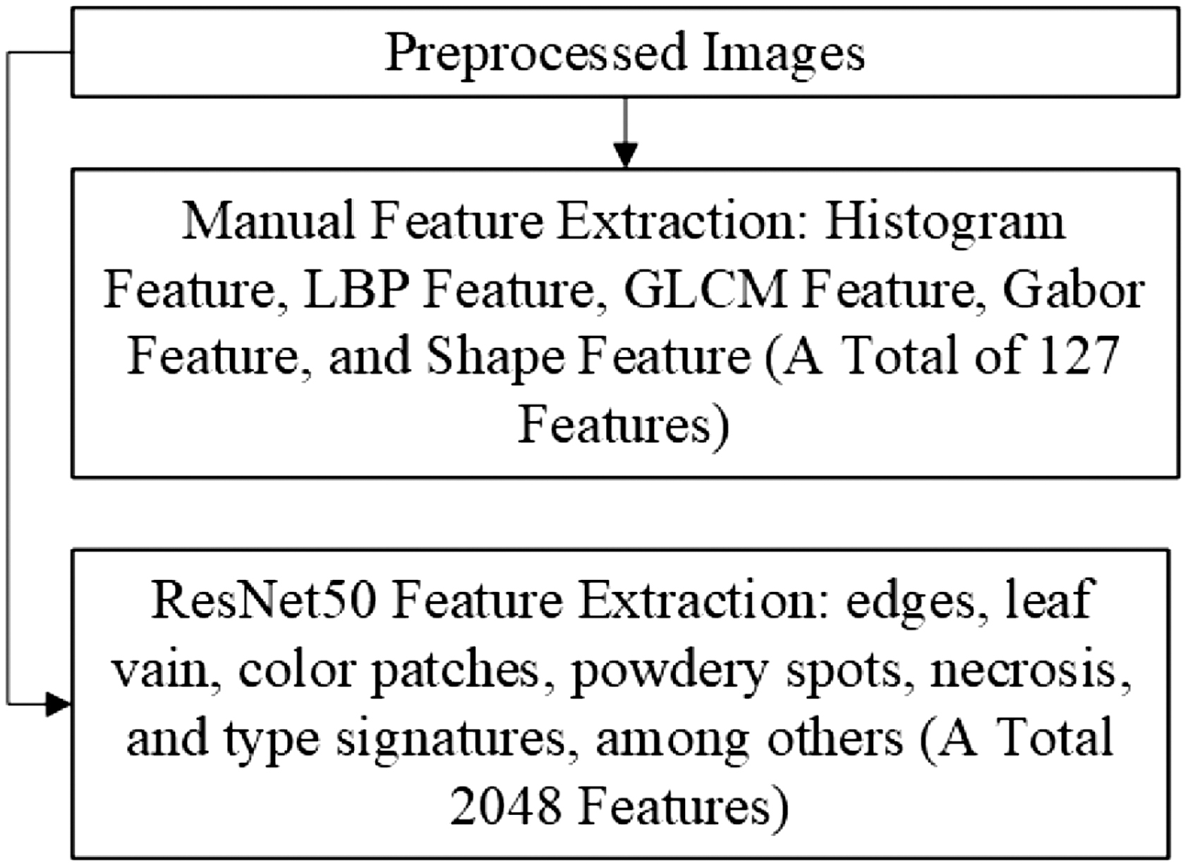
- 3.Feature extraction is performed solely for machine learning modeling, with the procedures conducted in two directions. One involves extractions where features are chosen manually. Selected features comprise histogram feature, Local Binary Pattern (LBP) feature, Gray Level Co-occurrence Matrix (GLCM) feature, Gabor features, and shape features. The second extraction is performed automatically with a pretrained model, ResNet50. In deep learning and YOLO training, features are automatically extracted.
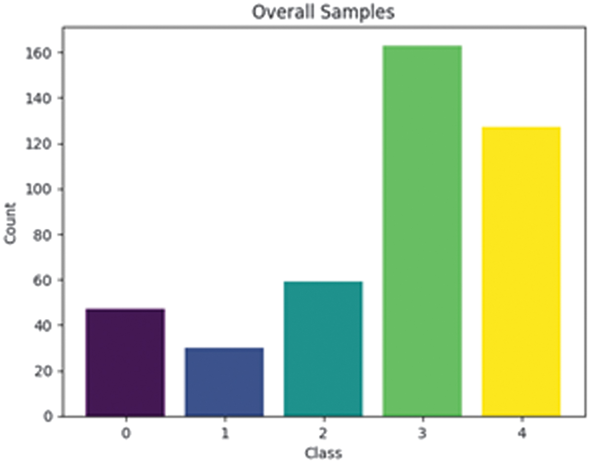
- 4.Data imbalance management occurs when the data acquired from sources exhibit imbalance conditions. The quantities of samples for Class 0, 1, and 2 are significantly lower than those of the other two classes. To achieve this, the balanced class weight method is utilized for modeling in machine learning and deep learning. Data augmentation is utilized for YOLO learning.
- 5.Various techniques are utilized for modeling. In machine learning, methods such as ANN, DTs, GB, RF, XGB, LR, SVMs, and NB are utilized. In deep learning, CNN and a pretrained ResNet50 model are utilized. For YOLO training, YOLO5, YOLO8, and YOLO9 are examined. Parameter adjustments for the modeling are also implemented.
- 6.Performance evaluation of models is performed using metrics like accuracy, precision, recall, and F1-score. For YOLO, an extra metric known as mAP is computed.
IV.RESULT AND DISCUSSION
A.DATA DESCRIPTION
Image data was collected from multiple farming regions in China by a research group from the Faculty of Information Technology at Jilin University. The collected data consisted of 426 images across the following disease categories: Powdery with 163 images, Leafminer with 59 images, Scab with 127 images, Anthracnose with 30 images, and Healthy leaves with 47 images. The leaf images collected were all taken in actual environments featuring intricate backgrounds, except for the melon leaves affected by scab disease, which were not photographed in a real setting but rather against a white background. Fig. 2 illustrates the class distribution within the dataset.
The dataset was divided for modeling using the Stratified K-Fold approach, with five sets of splits. Balanced class weight was utilized for the training dataset to prevent data imbalance during the training process.
B.PREPROCESSING AND FEATURE EXTRACTION
1).PREPROCESSING IMAGES
Utilizing the attributes of melon leaves and to effectively achieve the desired features, image preprocessing was performed. The preprocessing performed involves background removal, image cropping, contrast enhancement, normalization, and resizing. Flow of image preprocessing is shown in Fig. 3.
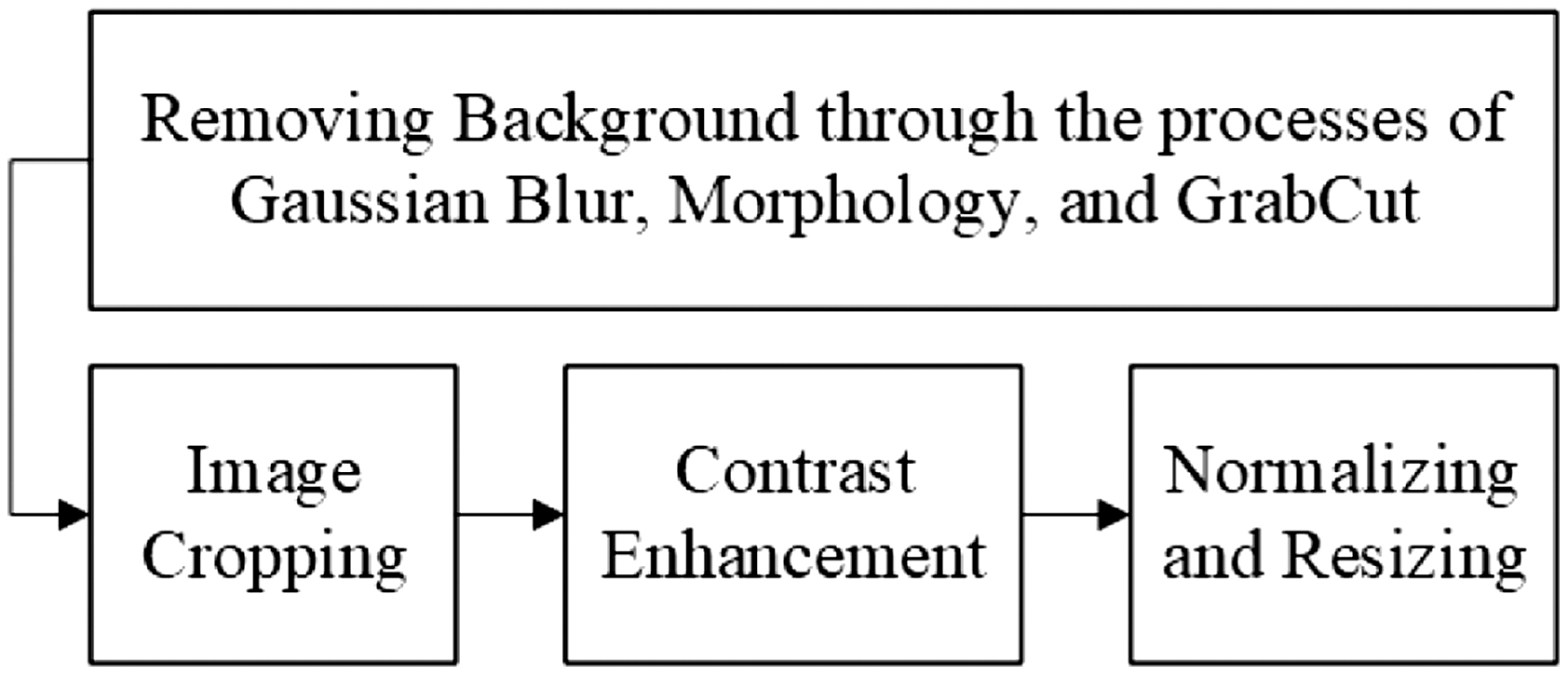 Fig. 3. Image preprocessing flow.
The removal of the background was applied because the acquired image data includes several types of backgrounds like soil, white template backgrounds, floors, and more. Background removal was achieved by initially applying Gaussian blur with a (5 × 5) kernel size, followed by contrast enhancement using CLAHE, masking for a broad spectrum of green hues, contour detection, morphology close with a (5 × 5) kernel size, and GrabCut techniques. These procedures were carried out to ensure that the background can be ideally distinguished from the leaf object.
Image cropping was performed since numerous leaf objects have extensive backgrounds surrounding the leaf itself. This method aims to prevent distractions caused by excessive learning from the background. Contrast enhancement was performed using CLAHE, since the diseases on the leaf frequently manifest as very subtle. Implementing the process was anticipated to enhance the recognition of leaf sections indicative of the diseases.
Normalization was performed to ensure that the coloring was adjusted within the range. The values for the normalization procedure were established to range from 0 to 255, and the technique utilized was min-max normalization. Resizing was performed to adjust the images to a uniform size for modeling purposes. In this study, the dimension utilized for the modeling was 128x128. Figure 4 illustrates a sample outcome of image preprocessing.
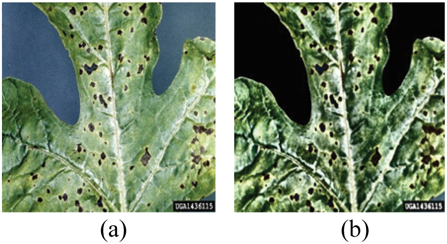 Fig. 4. (a) Resized original image and (b) preprocessed image.
2).FEATURE EXTRACTION
Feature extraction was performed for a selection of manually chosen features. They included histogram features made up of 32 bins for 3 RGB colors, LBP features that include 10 characteristics, GLCM with 5 characteristics, Gabor features consisting of 12 parameters, and shape features that comprise 4 parameters. A total of 127 features were extracted in a manual setting. Figure 5 shows two types of extractions conducted in this study.
3).FEATURE EXTRACTION USING DEEP LEARNING
In addition to manually set features, deep learning-based feature extraction was also performed. ResNet50 was employed to automatically derive features from the image. The initial weights for ResNet50 were derived from ImageNet, which contained 1.2 million natural images across 1000 categories.
For feature extraction, ResNet50 converted pixels into advanced features. Extracted features consisted of edges, leaf veins, color patches, powdery spots, necrosis, and disease-type markers. A total of 2048 features were extracted from the image. The parameters for ResNet50 extraction were weights = ‘imagenet’, include_top = False, and pooling = ‘avg’.
4).PREPROCESSING AND FEATURE EXTRACTION FOR YOLO
For YOLO, the dataset included 426 images, labeled for class identification. Annotation for object detection modeling involved identifying the bounding box for detection and classifying the object. The procedures utilized a pretrained model for Anthracnose disease and Healthy category since the model was accessible, while the other three were configured manually.
The annotation outcomes produced a final dataset comprising 869 images. The annotation results yielded class categories comprising 94 images for the healthy category, 341 images for the Anthracnose disease category, 99 images for the Leafminer disease category, 137 images for the Powdery disease category, and 198 images for the Scab disease category.
This labeled data with annotations and bounding boxes for object detection has experienced multiple phases of preprocessing and augmentation, such as resizing, blurring, rotating, flipping, and brightness. Figure 6 shows the flow of preprocessing and annotation conducted for the YOLO learning. The image in Fig. 7 is an example of an image that has been preprocessed, augmented, labeled, and had bounding box configurations applied.
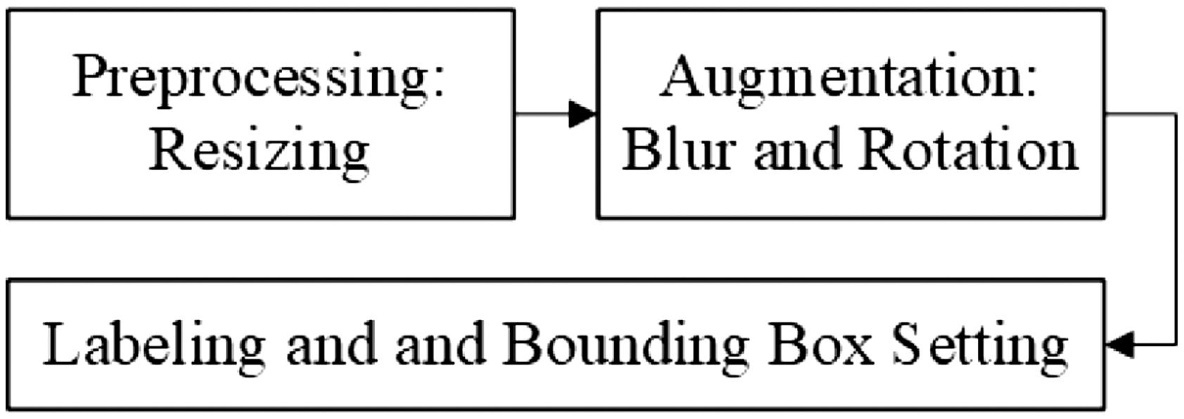 Fig. 6. Data preparation of YOLO object detection.
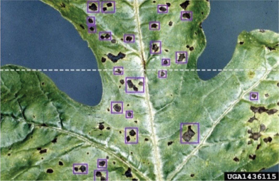 Fig. 7. Preprocessed, augmented, labeled, and box-bounded image example.
The settings used in preprocessing, augmentation, and labeling were as follows: resize fit within 640 × 640, horizontal and vertical flip, −90 degrees rotation (clockwise, counterclockwise, and upside down), rotation between −13 and + 13 degrees, brightness between −25% and + 25%, and blur up to 4.9 px.
C.COMPARISON OF MODELING RESULTS
1).MODELING USING SUPERVISED MACHINE LEARNING
Two datasets were considered in machine learning modeling. They created models utilizing features derived from manual adjustments and those elicited from the pretrained ResNet50 model. Table I displays the configuration settings for both models across eight distinct machine learning techniques.
Table I. Parameters set for supervised machine learning modeling
| Methods | Manually set extracted features | ResNet50-based extracted features |
|---|---|---|
| ANN | hidden_units = 16, learning_rate = 0.01, batch_size = 16, epochs = 50 | hidden_units = 16, learning_rate = 0.01, batch_size = 16, epochs = 100 |
| DT | max_depth = 4 | max_depth = 4 |
| GB | n_estimators = 100, learning_rate = 0.1, max_depth = 4 | n_estimators = 150, learning_rate = 0.1, max_depth = 2 |
| LR | penalty = ’l1’, C = 1.0, solver = ’liblinear’ | penalty = ’l2’, C = 0.01, solver = ’lbfgs’ |
| NB | var_smoothing = 1e-7 | var_smoothing = 1e-9 |
| RF | n_estimators = 100, max_depth = 8 | n_estimators = 50, max_depth = 3 |
| SVM | kernel = ’rbf’, C = 10, gamma = 0.01 | kernel = ’rbf’, C = 0.1, gamma = ‘scale’ |
| XGB | n_estimators = 50, learning_rate = 0.1, max_depth = 3 | n_estimators = 100, learning_rate = 0.05, max_depth = 2 |
Table II presents the metric outcomes of the examined modeling, encompassing accuracy, precision, recall, and F1-score, along with the confidence interval for accuracy based on features obtained through manual setting. The results indicated that SVM and XGB achieved higher accuracies than the other methods, reaching 77.9% and 78.6%, respectively.
Table II. Metrics of modeling results using various machine learning methods for manually set feature extraction
| Methods | Accuracy | CI lower | CI upper | Precision* | Recall* | F1-score* |
|---|---|---|---|---|---|---|
| ANN | 0.702 | 0.605 | 0.799 | 0.676 | 0.675 | 0.652 |
| DT | 0.596 | 0.493 | 0.700 | 0.567 | 0.562 | 0.542 |
| GB | 0.545 | 0.439 | 0.650 | 0.588 | 0.565 | 0.511 |
| LR | 0.749 | 0.657 | 0.841 | 0.702 | 0.654 | 0.661 |
| NB | 0.761 | 0.670 | 0.851 | 0.701 | 0.669 | 0.674 |
| RF | 0.754 | 0.662 | 0.845 | 0.690 | 0.627 | 0.633 |
| SVM | 0.779 | 0.692 | 0.867 | |||
| XGB | 0.725 | 0.696 | 0.699 |
*Macro average.
Table III displays the precision per class of modeling utilizing different machine learning techniques for features obtained through a manual configuration. The findings indicated that class 4 (Scab) achieved higher accuracies than the other classes. Class 0 (Health) exhibited poor accuracies across all the techniques. The limited amount of data for the category made it understandable, as the appearance of a Healthy leaf resembled those of Class 2 (Leafminer) and Class 3 (Powdery) diseases.
Table III. Per-class precision of modeling results using various machine learning methods for manually set extracted features
| Methods | 0 | 1 | 2 | 3 | 4 |
|---|---|---|---|---|---|
| ANN | 0.294 | 0.753 | 0.563 | 0.978 | |
| DT | 0.197 | 0.703 | 0.388 | 0.602 | 0.947 |
| GB | 0.198 | 0.750 | 0.360 | 0.739 | 0.892 |
| LR | 0.284 | 0.695 | 0.680 | 0.976 | |
| NB | 0.322 | 0.736 | 0.729 | 0.754 | 0.963 |
| RF | 0.250 | 0.785 | 0.678 | 0.963 | |
| SVM | 0.798 | 0.756 | 0.774 | ||
| XGB | 0.328 | 0.808 | 0.768 | 0.740 | 0.984 |
Table IV presents the metric outcomes of the analyzed modeling for features obtained via ResNet50. The findings indicated that every approach achieved accuracies of 96.3% or higher. Some even achieved flawless accuracy of 100%. They included GB, NB, RF, and SVM.
Table IV. Metrics of modeling results using various machine learning methods for feature extracted using pretrained model ResNet50
| Methods | Accuracy | CI lower | CI upper | Precision* | Recall* | F1-score* |
|---|---|---|---|---|---|---|
| ANN | 0.963 | 0.928 | 0.997 | 0.925 | 0.938 | 0.929 |
| DT | 0.995 | 0.986 | 1.004 | 0.993 | 0.995 | 0.993 |
| GB | ||||||
| LR | 0.988 | 0.968 | 1.008 | 0.981 | 0.975 | 0.977 |
| NB | ||||||
| RF | ||||||
| SVM | ||||||
| XGB | 0.986 | 0.967 | 1.005 | 0.985 | 0.966 | 0.973 |
*Macro average.
Table V displays the precision per class for modeling using features extracted from ResNet50. Alongside other metrics, per-class precision demonstrated high accuracy levels, with the lowest being ANNs for Class 1 (Anthracnose), which has a precision of 80%.
Table V. Per-class precision of modeling results using various machine learning methods for feature extracted using pretrained model ResNet50
| Methods | 0 | 1 | 2 | 3 | 4 |
|---|---|---|---|---|---|
| ANN | 0.944 | 0.800 | 0.933 | 0.949 | |
| DT | 0.971 | 0.993 | |||
| GB | |||||
| LR | 0.943 | 0.968 | 0.994 | ||
| NB | |||||
| RF | |||||
| SVM | |||||
| XGB | 0.937 | 0.988 |
These results demonstrated that features obtained through ResNet50, totaling 2048 features, better represented the image data than the alternative configurations. The variations in accuracy between the two configurations reached 40%–60%.
2).MODELING OF DEEP LEARNING
For modeling with CNN, the experiments were carried out employing two approaches. They were modeling with the original images and modeling with images that have undergone preprocessing. Two varieties of CNN were utilized. They consisted of pure CNN and CNN integrated with ResNet50. The parameters employed in CNN and CNN-ResNet50 are shown in Table VI.
Table VI. Parameters setting for deep learning modeling
| Methods | Parameter setting |
|---|---|
| CNN | Batch_size = 8, epochs = 30, filters = 32, dense_units = 128, dropout_rate = 0.5, kernel_size = 3, learning_rate = 0.0005 |
| CNN-ResNet 50 | Batch_size = 8, epochs = 30, filters = 32, dense_units = 128, dropout_rate = 0.5, learning_rate = 0.0005 |
The results from the modeling, as presented in Table VII, indicated that ResNet50 yielded improved outcomes when images were preprocessed initially. Nevertheless, the outcomes remained less favorable than the accuracies achieved by modeling machine learning techniques based on features extracted using the pretrained ResNet50 model.
Table VII. Metrics of modelling results using deep learning methods
| Methods | Accuracy | CI lower | CI upper | Precision* | Recall* | F1-score* |
|---|---|---|---|---|---|---|
| Original-CNN | 0.709 | 0.614 | 0.783 | 0.657 | 0.584 | 0.585 |
| Processed-CNN | 0.587 | 0.484 | 0.690 | 0.509 | 0.452 | 0.442 |
| Original-ResNet50 | 0.805 | 0.721 | 0.889 | 0.782 | 0.786 | |
| Processed-ResNet50 | 0.797 |
*Macro average.
Table VIII displays the precision for each class in the modeling with deep learning. Similar to modeling with machine learning techniques, Class 0 (Health) yielded the lowest accuracies, followed by Class 2 (Leafminer) and Class 3 (Powdery). The three classes shared nearly identical structures, making it quite difficult to distinguish between them. Nonetheless, these findings also indicated that CNN and ResNet50 were unable to achieve improved per-class precision in comparison to machine learning, where features were derived using ResNet50.
Table VIII. Per-class precision of modeling results using various machine learning methods for feature extracted using pretrained model ResNet50
| Methods | 0 | 1 | 2 | 3 | 4 |
|---|---|---|---|---|---|
| Original-CNN | 0.176 | 0.520 | 0.658 | 0.966 | |
| Processed-CNN | 0.272 | 0.613 | 0.314 | 0.592 | 0.754 |
| Original-ResNet50 | 0.398 | 0.910 | 0.809 | 0.794 | |
| Processed-ResNet50 | 0.938 | 0.951 |
3).MODELING OF YOLO LEARNING
Modeling was conducted for the three YOLO types, that is YOLOv5, YOLOv8, and YOLOv9, using 869 annotated image data. Modeling was performed with different configurations, including the available variations for each YOLO and the input data’s image sizes. The types of YOLO employed were YOLO Large and YOLO Small, while the image dimensions utilized were 480 and 768 pixels. The parameters utilized in YOLO modeling were batch = 8, lr0 =0.0005, lrf = 0, warmup_epochs = 5, patience = 50, os_lr =True, optimizer = AdamW, amp = True, and save_period = 10. The outcomes of the modeling with YOLOv5, YOLOv8, and YOLOv9 are presented in Table IX.
Table IX. Results of object detection of melon plant diseases using YOLO
| YOLO | mAP50-95 | Precision | Recall | F1-score | Accuracy |
|---|---|---|---|---|---|
| V5 | 0.51156 | 0.6884 | |||
| 0.6718 | 0.6634 | 0.6658 | |||
| V9 | 0.51566 | 0.6481 | 0.6605 | 0.6510 | 0.6836 |
According to the modeling outcomes, YOLOv8 achieved the highest average accuracy at 70%, while YOLOv5 presented the top average precision, recall, and F1-score at 69%, 67%, and 68%, respectively. YOLOv8 generated higher accuracy of 70% and a marginally higher mAP50-95 than the other YOLO versions, achieving a value of 53%. This indicates that merely 53% of the entire testing data has been accurately recognized along with their respective locations.
These modeling outcomes exhibit reduced accuracy, precision, recall, and F1-score compared to modeling with deep learning employing a pretrained ResNet50 model. The precision of modeling with YOLO was still inferior to that of various modeling techniques utilizing supervised machine learning methods like ANN, LR, XGB, RF, and many others.
A.DISCUSSION
This research examined various techniques to assess the variations in the generated models by analyzing multiple evaluation metrics such as accuracy, precision, recall, and F1-score. In general, various techniques can be employed to identify diseases in melon plants using images of their leaves.
According to the findings, models created with machine learning techniques that utilized feature extraction from the predefined ResNet50 model exhibited greater accuracy than alternative approaches. In certain machine learning techniques, the accuracy achieved a value of 100%. Results for precision per class also exhibited comparable trends. This has further demonstrated that the combination might be the optimal approach for modeling melon leaf disease. To analyze further, the disparity of these results compared to the accuracies of modeling using features extracted with manual settings reached as much as 30%–50%. The quantity of features extracted to represent the images affected the modeling substantially. These results indicated that ANN had the poorest performance compared to the others.
Upon comparing the modeling outcomes from original images versus preprocessed images, no distinct pattern emerged. This may be influenced by the quality of data that could offer advantages between the different models. The application of ANN for classification might also create an impact, as demonstrated in machine learning evaluations, with ANN showing the poorest performance compared to other techniques. Nonetheless, CNN using the pretrained ResNet50 model outperformed the traditional CNN setup.
Modeling with YOLO has produced unsatisfactory outcomes, with accuracy levels between 68% and 70%. This remained distant from the accuracy obtained through machine learning with features extracted by ResNet50. This may happen because the processes of labeling and bounding boxes still need unique attention. The manual labeling and bounding box processing could have influenced the modeling outcomes. At present, the process of labeling and setting bounding boxes with pretrained models was not all possible, as pretrained models for various melon leaf diseases have yet to be developed. Another issue with the YOLO modeling was the unresolved data imbalance, despite the application of augmentation.
B.RECOMMENDATION
According to the research findings, utilizing machine learning with image features obtained from the pretrained ResNet50 model is advisable for this case, as the modeling achieved 100% accuracy for certain methods, and nearly 100% accuracy for others. Of the various methods, GB, NB, RF, and SVM yielded the most favorable outcomes. In the modeling that utilized features obtained through manual configuration, additional types of features could be incorporated to explore a wider range of variations present in the images involved in the modeling.
Regarding CNN, a more extensive modeling approach through parameter adjustments could be applied across a broader set of values, allowing for the selection of parameters that are appropriate for the specific case. For YOLO modeling, additional exploration is required, particularly regarding annotation and bounding box configuration. A predefined model for image annotation and bounding box placement must ensure high accuracy, and for those not yet modeled, the process quality could be enhanced. Given YOLO’s capability for object detection through image segments, it is valuable to pursue additional research on detecting melon plant diseases using YOLO. This is vital, as YOLO closely mimics the way humans recognize plant diseases.
V.CONCLUSIONS
Multiple conclusions were derived from the research:
- 1.Machine learning, deep learning, and YOLO could identify diseases in melon plants by analyzing their leaves. Each method’s application possessed distinct traits that affected the modeling process, encompassing preprocessing, feature extraction, augmentation, labeling, bounding box configuration, and others.
- 2.The precision of machine learning models utilizing features derived from the predefined ResNet50 model was superior to the alternatives. Certain machine learning techniques could reach up to 100% accuracy. This environment was highly advisable for this situation. The suggested methods included GB, NB, RF, and SVM.
- 3.More investigation into different contexts, including incorporating suitable preprocessing, enhancing feature extraction with more features, varying augmentations, improving labeling accuracy, adjusting bounding box settings, and fine-tuning parameters for modeling, requires exploration. This is essential for techniques that have demonstrated effective outcomes and approaches that hold promise for additional enhancement, like CNN and YOLO.