I.INTRODUCTION
Through the application of machine learning, sentiment analysis has proven to be one of the most successful areas in determining a wide range of outcomes from a variety of perspectives. On the other hand, research communities overlooked the possibility of taking into account sentiment based on locations or geographical boundaries. In a similar vein, taking into account the fact that human beings are the result of a combination of inherited characteristics and environmental influences, it is important to justify the reason why, despite the fact that numerous research studies have been conducted in the field of sentiment analysis, there has been a lack of focus on the application of geographical regions. This is the reason why the current study proposed to investigate enhanced sentiment analysis toward specific locations and neighborhoods using advanced machine learning techniques.
Existing aspect-based sentiment analysis (ABSA) approaches predominantly emphasize transformer-based contextual encoders without addressing interpretability and probabilistic reasoning. Moreover, many studies overlook the structured dependency between geographic entities and aspect categories. This creates a gap in understanding how location-linked sentiment structures can be probabilistically modeled rather than purely sequentially learned.
Within the domain of aspect-based sentiment analysis (ABSA), earlier studies [1–9] have explored various machine learning and deep learning techniques for sentiment classification tasks. Various classifiers, including logistic regression (LR), gradient boosting (GB), support vector machines (SVM), and Bayesian networks, have been extensively employed to address tasks similar to those under current investigation. The aim of our study is to explore this area through a thorough comparative analysis between our models and the established benchmarks. The approaches exhibiting the highest performance are incorporated within the models that are undergoing comparison with each other.
In the field of sentiment analysis, this is considered the standard approach that is directly linked to the linear classification algorithm. Given its relative simplicity compared to deep learning models, linear regression proves to be effective in uncovering various baseline models related to text classification. Linear regression can be a complex technique, though not as intricate as deep learning; nonetheless, it remains effective. In ABSA, LR can be employed to forecast the sentiment labels associated with particular attributes or entities extracted from the text. In a similar vein, these predictions can be formulated concerning the manner in which the texts are sourced, given that texts can originate from various heterogeneous sources. The predictions are based on the characteristics obtained from the textual data [10]. Another significant classifier is the “Gradient boosting algorithms” such as XGBoost, LightGBM, and CatBoost, which are being increasingly employed in natural language processing tasks. A typical scenario encompasses the foundational tasks conceptualized in ABSA, which is a crucial component of the system involved in numerous natural language processing tasks. Given these considerations, and recognizing the importance of reliability in a prediction model, it is essential and aligns with the fundamental principles of boosting algorithms. Thus, they will effectively address the core elements of prediction [11].
In the context of a directed acyclic graph, often known as a Bayesian network, there exists a derivation related to the probabilistic relationships among variables in this scenario. The methodology utilizes conditional probability in conjunction with a network framework to illustrate the interrelationships among variables [12,13]. Bayesian networks model probabilistic dependencies among variables, enabling effective representation of relationships between entities, aspects, and contextual sentiment features. This section presents a comprehensive examination of the differential current (Id) and the through current (It). Networks, categorized as a type of architecture within recurrent neural networks (RNNs), have been widely utilized in natural language processing tasks, including sentiment analysis and ABSA. The use of long short-term memory (LSTM) networks proves to be a highly effective method for performing aspect-level sentiment analysis in ABSA by identifying entities or components within the text and subsequently connecting those components to emotions [14].
GRU is a variant of LSTM algorithm, representing a fundamental type of RNN that integrates gating mechanisms. GRUs excel at recognizing long-range dependencies in sequential data, while LSTMs often face challenges in this area. These models excel in sentiment analysis tasks within ABSA, demonstrating a strong capability in handling sequential text data. The GRU neural network functions in a cyclical fashion, leveraging both the current input and past output data to ascertain the current output. The investigation carried out by Li et al. in 2020 demonstrates that the output at any given moment is shaped by the prior information. This feature makes it especially suitable for tasks that involve sequential labeling, like the segmentation of Chinese words.
This investigation is notable for its examination of the geographic emphasis in sentiment analysis, an area that is still quite innovative, especially within the field of urban sentiment mining. The methodology utilizes established models including LR, GB, LSTM, and Bayesian networks, with the innovative aspect being its specific application to geospatial opinion mining through a QA-based dataset. This study effectively connects sentiment classification with particular neighborhood characteristics, offering valuable insights for practical applications in areas like urban planning, tourism development, and community involvement.
Unlike prior studies that primarily focus on improving contextual encoders or transformer-based architectures, this work investigates the comparative behavior of probabilistic graphical models and deep sequential models under a geospatially constrained aspect-based sentiment setting. Specifically, we analyze whether conditional dependency modeling via Bayesian networks offers advantages over sequential neural architectures when aspects are tied to location entities. The contribution of this study lies not in introducing a new dataset but in providing a probabilistic interpretability perspective and rigorous comparative evaluation under statistical testing.
The remainder of this paper is organized as follows. Section II presents a review of related work in ABSA, geospatial sentiment mining, and transformer-based models. Section III describes the proposed methodology, including data preprocessing, feature engineering, and model configuration. Section IV reports the experimental results, comparative evaluation, and statistical validation. Section V discusses the findings and their practical implications. Finally, Section VI concludes the paper and outlines directions for future research.
II.METHODOLOGY
A wealth of previous studies has been conducted in the areas of sentiment analysis and machine learning [1–3,5–9,15–20]. This study showcases the application of machine learning techniques to the SentiHood dataset for the purpose of categorization. Our focus lies in the development of the previously outlined concepts in the introduction. This is depicted in Fig. 1. The dataset was obtained from Kaggle and then processed to remove any inconsistencies or errors. Following preprocessing, LR, BN, and GB, together with the deep learning models LSTM and GRU, were implemented and evaluated for sentiment classification. We evaluated the effectiveness of the deployed models by analyzing their accuracy, precision, recall, and F1-score.
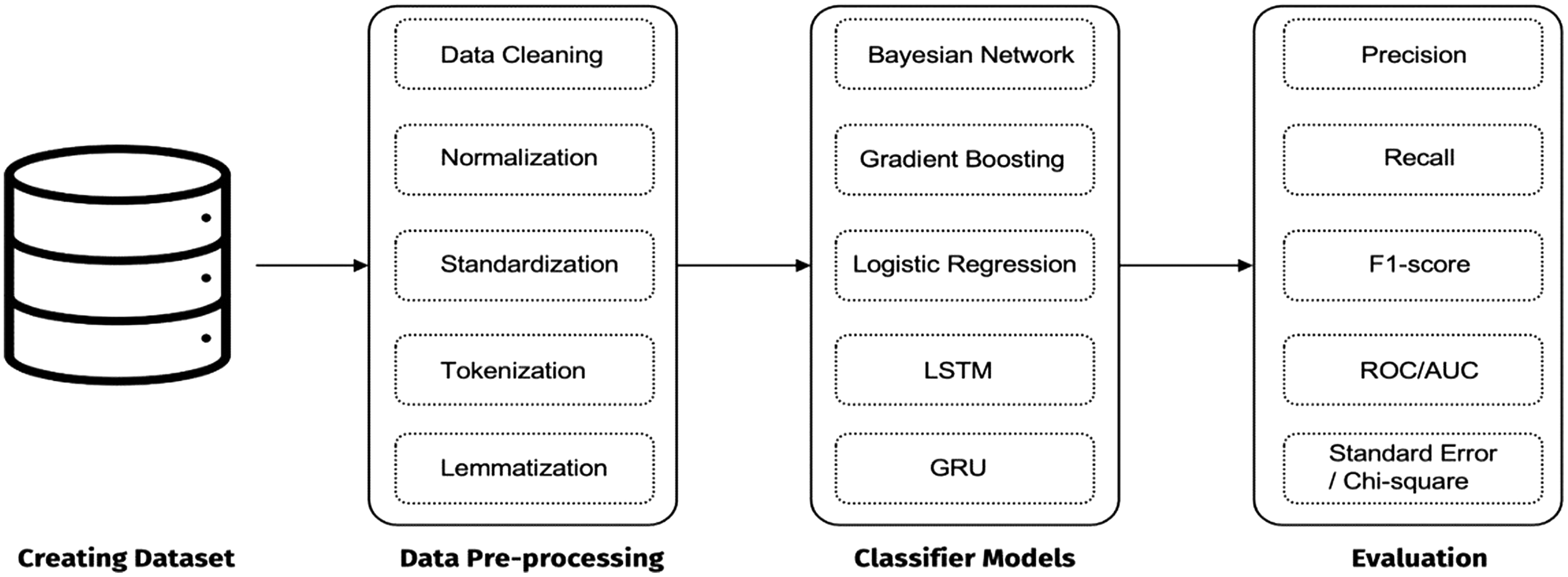 Fig. 1. Expanded methodological workflow including preprocessing, feature extraction, model training, hyperparameter tuning, and statistical validation.
The SentiHood dataset was cleaned by removing HTML tags, special characters, and redundant whitespace. Text was lowercased and tokenized using the NLTK tokenizer. Stopwords were removed for classical models (LR, GB, and BN), while deep learning models retained full sequences. For LR and GB, TF-IDF features (unigram + bigram) were extracted with a vocabulary size capped at 10,000 terms. For Bayesian network modeling, categorical features were constructed including Entity, Aspect, Sentence1 token group, Sentence2 token group, and Chi-square, and G-square tests were applied for variable selection. For the LSTM and GRU models, the word embedding dimension was set to 100, the maximum sequence length to 100, dropout to 0.5, the Adam optimizer was used for training, and the models were trained for 20 epochs with early stopping based on the development-set F1-score.
The dataset preprocessing pipeline was designed to ensure consistency, reproducibility, and model robustness. Initially, raw text instances were cleaned by removing HTML tags, special characters, and redundant whitespace. All text was converted to lowercase to reduce lexical sparsity. Tokenization was performed using the NLTK word tokenizer. For classical machine learning models (LR and GB), English stopwords were removed to reduce noise, whereas deep learning models (LSTM and GRU) retained full sequences to preserve contextual dependencies. For sequential models, sentences were padded or truncated to a maximum sequence length of 100 tokens to ensure uniform input dimensions. Stratified sampling was applied during dataset partitioning to preserve class distribution across splits.
Feature engineering differed across model categories. For LR and GB, textual data were transformed using TF-IDF vectorization with unigram and bigram features, and the vocabulary size was capped at 10,000 tokens to prevent overfitting and excessive dimensionality. L2 regularization was applied to LR. For the Bayesian network, categorical features were constructed, including entity, aspect category, and sentence-level token groupings (Sentence1 and Sentence2). Feature relevance was evaluated using Chi-square and G-square statistical tests, and only statistically significant variables were retained. The Bayesian network structure was learned using a score-based hill-climbing algorithm with Bayesian information criterion (BIC) scoring, while parameters were estimated using maximum likelihood estimation.
Deep learning models were implemented with an embedding layer of dimension 100 and 128 hidden units. A dropout rate of 0.5 was applied to reduce overfitting. Models were trained using the Adam optimizer with a learning rate of 0.001 for up to 20 epochs. Early stopping with a patience of three epochs was applied based on development set F1-score to prevent overfitting. In addition, a BERT-base-uncased transformer model was fine-tuned for comparison using a learning rate of 2e-5, batch size of 16, maximum sequence length of 100, and three training epochs.
The dataset was partitioned into 70% training, 10% development, and 20% testing sets using stratified sampling. The development set was exclusively used for hyperparameter tuning, threshold optimization, and early stopping decisions, while the test set remained completely unseen until final evaluation. To ensure robustness, five-fold cross-validation was performed, and paired t-tests were conducted to assess statistical significance between models. Additionally, bootstrap resampling with 1,000 iterations was applied to compute 95% confidence intervals. All experiments were conducted with a fixed random seed of 42 to ensure reproducibility.
III.DATASET, EXPERIMENTAL, AND RESULT
SentiHood is a dataset created for focused ABSA, derived from the Yahoo! Answers question-and-answer platform. The dataset is concentrated on inquiries pertaining to neighborhoods in London. The data were sourced from Kaggle and compiled into a unified CSV file to enhance usability, facilitating both analysis and model training. The procedures for data preparation were designed to enhance the dataset, ensuring consistency, cleanliness, and readiness for analysis, while preserving its integrity for focused ABSA of neighborhoods in London [21].
The KS Cutoff line is set at the 0.5 threshold, demonstrating a specificity of 0.459 and a sensitivity of 0.812. To deem a model accurate, the receiver operating characteristic (ROC) curve should rapidly approach the top-left corner of the graph, where the 1–specificity differential is maximized. Figure 2 employs a ROC curve to assess a binary classification model by graphing sensitivity (true positive rate) in relation to 1–specificity. The blue curve illustrates the model’s effectiveness in differentiating between favorable and unfavorable outcomes across various thresholds. The diagonal black line illustrates a random or stochastic model. The sensitivity of this model is calculated as one minus specificity, indicating that the classifier is limited to making educated guesses.
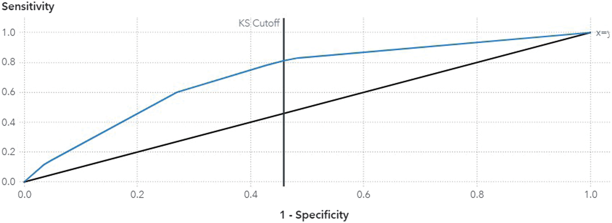
The blue ROC curve is positioned above the diagonal line, signifying that the model demonstrates superior classification performance compared to random chance. The model demonstrates improved prediction and separation as the blue curve ascends and shifts left from the diagonal. In many prediction tasks, an initial steep slope enhances sensitivity while reducing false positives. The vertical “KS Cutoff” line represents the optimal cutoff point for the Kolmogorov–Smirnov (KS) test. The cumulative distributions of the positive and negative classes show the most significant differences in this context. This threshold indicates the optimal point at which the model can effectively distinguish between different elements. The classifier currently achieves the optimal balance between sensitivity and specificity in differentiating the two outcome groups. Figure 2 illustrates the trade-off between true positives and false positives in the predictive model. The blue ROC curve’s closeness to the top-left corner, along with the KS Cutoff, suggests that the model demonstrates strong discriminative ability. The figure illustrates the model’s reliability, demonstrating that its classification decisions effectively balance detection sensitivity with false alarm control.
Figure 3 demonstrates that at a threshold of 0.5, this model achieves an accuracy of 68%. The calculation involves dividing the total number of observations by the sum of true positives and true negatives. The evaluation of accuracy occurs at various cutoff points, measuring the proportion of observations correctly identified as events or non-events. The cutoff values rise in steps of 0.05, spanning from 0 to 1, inclusive. The model demonstrates a moderate accuracy of 0.53 when evaluated at lower cutoff values ranging from 0.0 to 0.2. The forecasts are well considered, though they are not without their imperfections. With an increase in the cutoff from 0.3 to 0.6, there is a rapid rise in accuracy, which stabilizes between 0.68 and 0.70. The model demonstrates optimal classification performance within this range. This represents the optimal threshold window for the model, where sensitivity and specificity are effectively aligned to enhance accuracy, resulting in a balanced count of true positives and negatives. Following a threshold of 0.6, there is a gradual decline in accuracy, suggesting that elevated thresholds lead to an increased misclassification of positive cases as negative. Following 0.75, the accuracy declines to below 0.55 and remains approximately at 0.50 until reaching 1.0. The predominant findings are negative, suggesting a cautious prediction bias. Figure 3 illustrates the significant impact of the cutoff on model accuracy. Determining the optimal threshold, typically ranging from 0.3 to 0.6, is essential for enhancing predictive performance. This image assists professionals in fine-tuning the classification model to achieve a balance between precision and recall, ensuring accurate prediction outcomes.
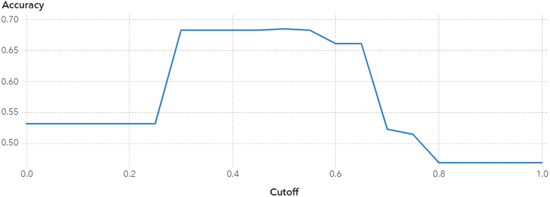
Figure 4 illustrates the impact of the F1-score and cutoff threshold on the predictions made by a binary classification model. The horizontal axis displays cutoff values ranging from 0.0 to 1.0. The vertical axis represents the F1-score, which is the harmonic mean of precision and recall. The F1-score effectively balances false positives and false negatives, rendering it a valuable metric for assessing models that have significant implications. The model demonstrates the ability to produce balanced predictions, maintaining an F1-score of approximately 0.65 within the lower cutoff range of 0.0 to 0.2, even when the majority of samples are positive. The F1-score reaches its highest point slightly above 0.70 as the cutoff increases from 0.3 to 0.6. This range seems optimal for achieving a balance between precision and recall in the model. Within this range, the classifier successfully identifies true positives while minimizing false positives, showcasing its effective predictive capabilities. Nonetheless, the F1-score declines rapidly, falling below 0.6, dipping near 0.4 around 0.7, and approaching zero as the cutoff nears 1.0. The abrupt decline is causing the model to exhibit increased bias toward negative classifications, resulting in the oversight of numerous positive cases (false negatives) and a reduction in recall. Figure 4 illustrates the significant impact of classification cutoff selection on the F1-score. The optimal threshold, typically ranging from 0.3 to 0.6, achieves a balance between true positives and false positives, thereby enhancing the model’s performance. This figure illustrates the importance of modifying the decision boundary to ensure the model performs effectively and maintains balance across various operational contexts.
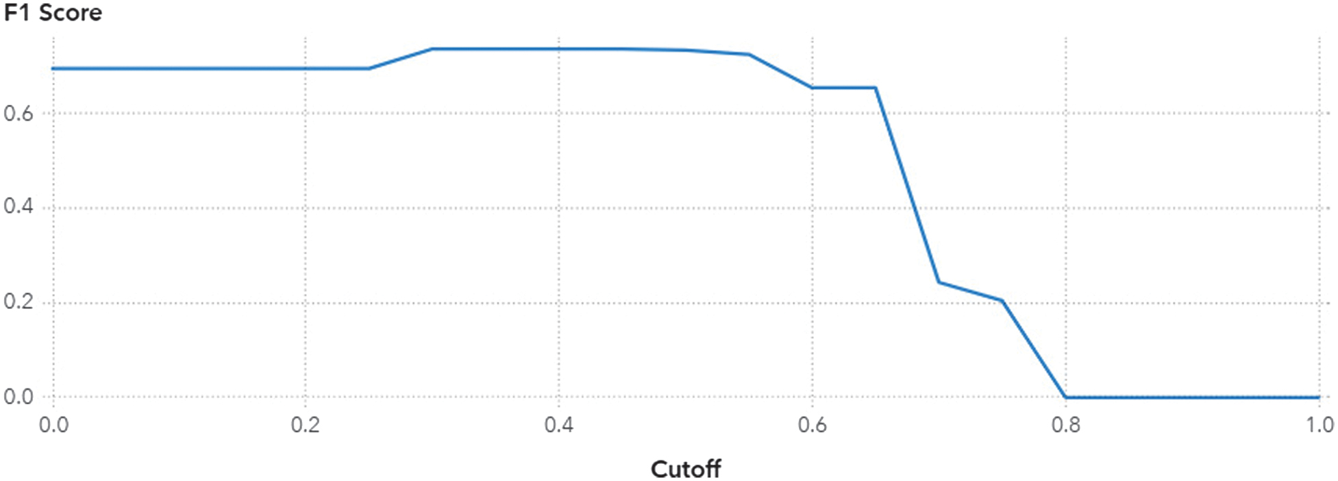
Table I presents the results of the Chi-square and G-square analyses for the entity, aspect, sentence2, and sentence1 variables. These tests assess the significance and strength of each variable in relation to the target outcome. The table includes columns for Chi-square values, p-values (Pr > Chi-square and Pr > G-square), G-square values, and degrees of freedom. All variables included are deemed “Selected,” indicating their statistical significance and retention in the final model. Under the assumption of independent frequencies, the Chi-square column illustrates the deviation of observed frequencies from the expected frequencies. Higher values suggest a more robust connection. Sentence1 exhibits the most significant Chi-square statistic at 2,355.2653, with sentence2 following at 472.8493, aspect at 431.7782, and entity at 48.1999. Sentence1 exerts the most substantial influence on the model’s predictive capability, with sentence2 and aspect following in importance, while entity, though having the least impact, remains significant. The p-values for all variables (Pr > Chi-square and Pr > G-square) are 0.0000 at the 99.9% confidence level, demonstrating a statistically significant relationship with the dependent variable. G-square statistics, which assess goodness-of-fit through likelihood ratios, produce results that are comparable to those of Chi-square. Results demonstrate consistency. The degrees of freedom column for each variable indicates the number of independent comparisons that can be made, for example, entity 1; sentence1 1,709. The elevated degree of freedom in Sentence1 suggests a more intricate structure or a greater number of levels analyzed. Table I indicates that all four variables demonstrate strong predictive capabilities. Sentence1 demonstrates the most significant statistical impact on the model, suggesting that the selected features effectively account for the data patterns.
Table I. BN variables selection
| Variable name | Selected | Chi-square | Pr > G-square | Pr > Chi-square | G-square ↑ | Degrees of freedom |
|---|---|---|---|---|---|---|
| Entity | Yes | 48.1999 | 0.0000 | 0.0000 | 49.3730 | 1 |
| Aspect | Yes | 431.7782 | 0.0000 | 0.0000 | 443.4599 | 3 |
| Sentence2 | Yes | 472.8493 | 0.0000 | 0.0000 | 489.5334 | 7 |
| Sentence1 | Yes | 2,355.2653 | 0.0000 | 0.0000 | 3,230.2970 | 1,709 |
Figure 5 illustrates a ROC curve, which displays sensitivity (true positive rate) in relation to 1–specificity in order to evaluate the diagnostic performance of a binary classification model. The blue curve illustrates the performance of the model across various thresholds. The diagonal black line illustrates a classifier that operates randomly or without skill, characterized by sensitivity equating to 1 minus specificity. This diagonal line illustrates a stochastic model that lacks the ability to differentiate. The blue ROC curve in this figure ascends rapidly and remains close to the upper-left corner, signifying robust classification capability. A curve positioned significantly above the diagonal suggests that a model is capable of effectively differentiating between positive and negative classes. The sharp increase at the beginning indicates a high level of sensitivity and a minimal occurrence of false positives, which is beneficial for the accuracy of predictive modeling and for early detection purposes. The model exhibits a minimal false positive rate and demonstrates a sensitivity close to 1.0, indicating near perfection. This indicates a strong predictive capability. The vertical “KS Cutoff” line indicates the optimal point of the KS statistic, representing the maximum distinction between the cumulative distributions of the positive and negative classes. This cutoff demonstrates the most significant difference between sensitivity and specificity. It achieves an optimal equilibrium between accurate identifications and erroneous alerts. Figure 5 illustrates the effectiveness of the classification model, as evidenced by the ROC curve’s proximity to the top-left corner and the elevated KS statistic. The KS Cutoff guarantees that the model maintains sensitivity while preserving specificity, aiding in the selection of the optimal threshold for operational deployment. Consequently, it attains the highest levels of predictive accuracy and dependability.
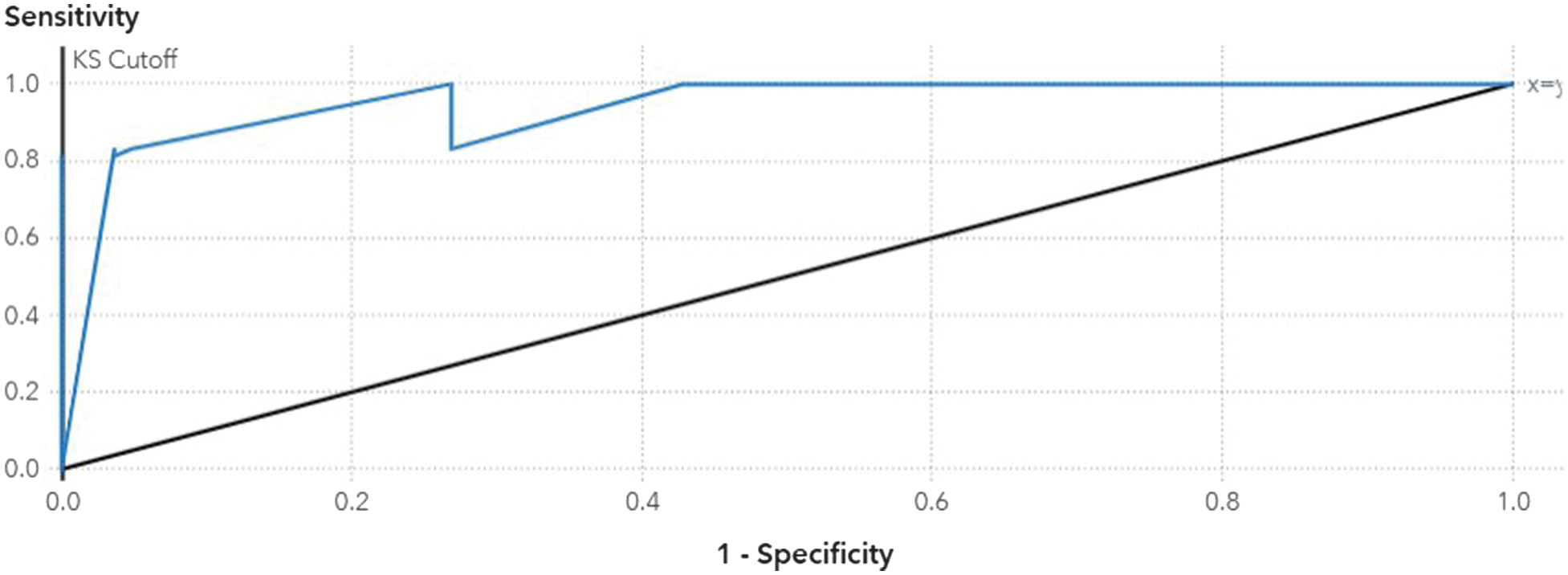
Figure 6 illustrates the impact of varying the cutoff threshold from 0.0 to 1.0 on the accuracy of the model. The horizontal axis illustrates the threshold value used for distinguishing between positive and negative predictions. The vertical axis represents the accuracy of the model. This plot is essential for identifying the threshold that optimizes predictive accuracy while avoiding overfitting or underclassifying the data. Low cutoff values ranging from 0.0 to 0.2 sustain an accuracy between 0.50 and 0.60. This indicates that the model struggles to differentiate between classes when the majority of its predictions are positive. As the cutoff surpasses 0.2, there is a rapid increase in accuracy, which then stabilizes within the range of 0.75 to 0.90. This section illustrates the model’s ideal equilibrium in identifying both positive and negative cases. The peak accuracy of the curve, 0.90, occurs at a cutoff between 0.45 and 0.65. This plateau represents the optimal performance of the model, characterized by a reduction in errors and effective generalization. The model exhibits excessive caution in identifying positive cases, leading to a rapid decline in accuracy beyond 0.7, which consequently increases the number of false negatives. The reduction continues until the accuracy nears random levels (approximately 0.50) at a threshold close to 1.0. Figure 6 demonstrates the impact of classification threshold on the accuracy of the model. Identifying the optimal cutoff range, typically falling between 0.4 and 0.6, is essential for enhancing model predictive performance. This figure assists data analysts and practitioners in fine-tuning model thresholds to ensure accuracy, reliability, and a balanced recall for real-world applications.
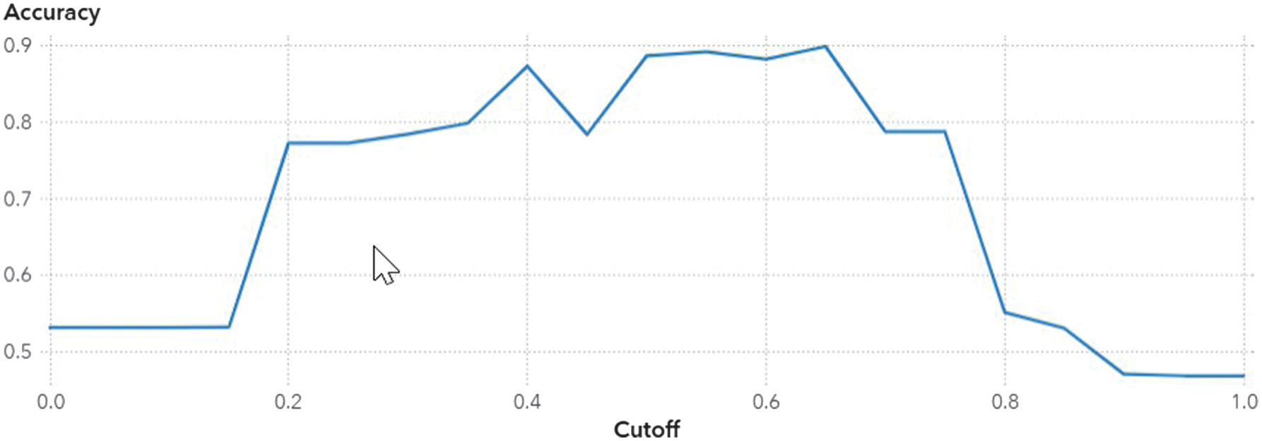
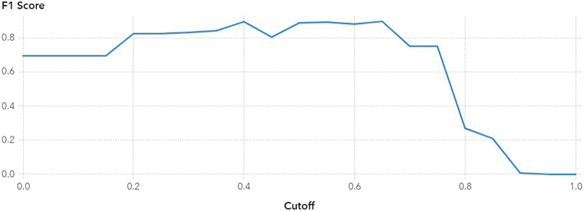
Figure 7 illustrates the relationship between the F1-score and the cutoff threshold in a binary classification model. The horizontal cutoff values range from 0.0 to 1.0, while the vertical F1-score represents the harmonic mean of precision and recall. The F1-score serves as a crucial metric for evaluating model performance, particularly when both false positives and false negatives can lead to significant repercussions. The accuracy of the two classes is evenly matched. In the lower cutoff range (0.0–0.2), the F1-score demonstrates a moderate level, falling between 0.65 and 0.70. The recall rate is elevated; however, the precision is lacking due to an excessive number of positive cases being incorrectly identified as positive. With an increase in cutoff from 0.25 to 0.6, the F1-score demonstrates a rise, stabilizing in the range of 0.85 to 0.90. The model demonstrates optimal performance and consistency within this range. This range achieves an optimal equilibrium between confirmed cases and false positives. Following 0.6, the F1-score experiences a gradual decline, which becomes more pronounced after 0.75, falling below 0.5 and nearing zero as it approaches 1.0. This significant decline suggests that the model is adopting a more cautious approach, resulting in fewer positive predictions and a decrease in recall. The F1-score significantly decreases when recall declines, despite a potential increase in precision for a limited number of true positives.
The quantity of trees within an ensemble learning model, like a Random Forest or Gradient Boosted Tree model, influences the average squared error (ASE). Refer to Fig. 8 for further details. The count of trees in the model is displayed on the left, ranging from 0 to 100. The ASE displayed on the right indicates that our predictions did not align with the actual outcomes, ranging from 0 to 100. Lower ASE values signify a model that is more precise and offers improved predictions. Beginning with fewer than 10 trees, the ASE stands at 0.24, indicating a significant level of error. Although patterns are readily identifiable, the model remains inadequately aligned with the data. A greater number of trees leads to a rapid decrease in error. This indicates that the group is enhancing its ability to connect input features with the intended outcomes. Between 10 and 30 trees, there is a notable decrease in ASE, suggesting a more stable and generalized model. Following the addition of 40 trees, the curve begins to stabilize. This indicates that an increase in trees does not provide assistance. This plateau indicates that the model has absorbed nearly all available knowledge, and incorporating additional individuals into the ensemble does not lead to a decrease in errors. The model demonstrates improvement as the ASE remains approximately 0.21 with 80 to 100 trees.
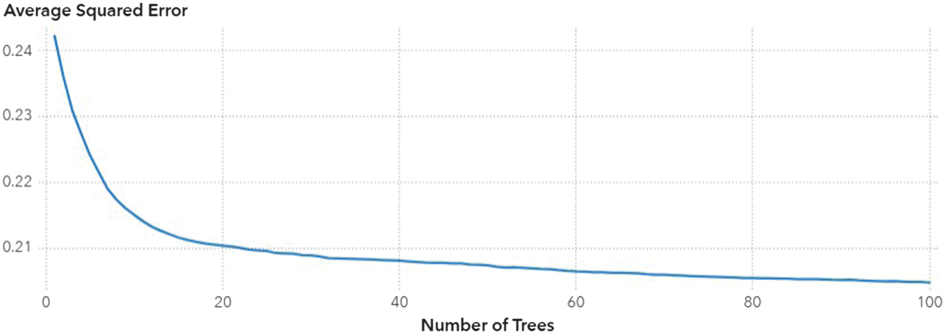 Fig. 8. Average squared error plot.
Figure 10 illustrates a ROC curve that depicts sensitivity (true positive rate) alongside 1–specificity (false positive rate) across various classification thresholds. The blue ROC curve illustrates the actual performance of the model, whereas the diagonal black line represents the sensitivity of a random or no-skill classifier, which is equal to one minus specificity. The performance aligns closely with that of random guessing when evaluated against this baseline. The blue curve exceeds the diagonal, demonstrating that the model surpasses a random classifier. A steeper ascent of the ROC curve toward the top-left corner indicates that the model is more effective in distinguishing between positive and negative cases. The blue curve in this figure demonstrates a high sensitivity and a low false positive rate, indicating its effectiveness in distinguishing between the two classes. The vertical “KS Cutoff” line represents the KS statistic. This represents the optimal cutoff point for the most significant cumulative distribution disparity between the positive and negative classes. At this threshold, the classifier achieves optimal separation, maximizing true positives while minimizing false positives. The KS statistic serves a crucial role in risk modeling and predictive analytics by identifying the optimal decision threshold. Figure 9 illustrates that the model performs effectively and demonstrates a strong ability to differentiate between various elements. The ROC curve and elevated KS separation point demonstrate that the model exhibits reliability and accuracy. The distinct separation from the diagonal baseline indicates that the classifier is capable of differentiating between classes, establishing it as a dependable predictive model for decision-making or practical applications.
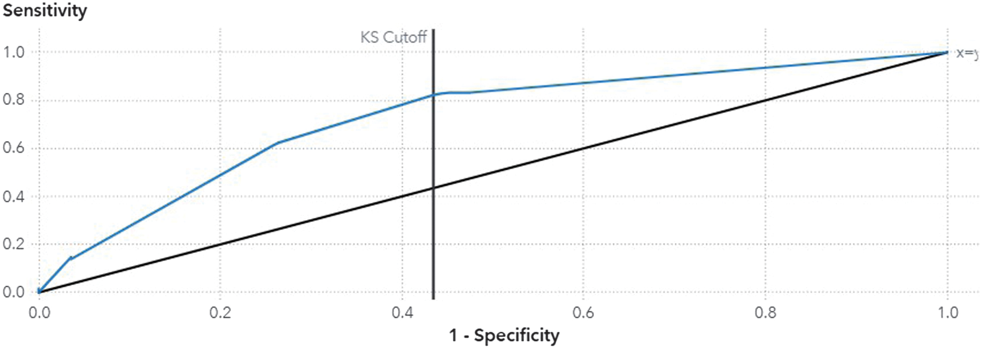
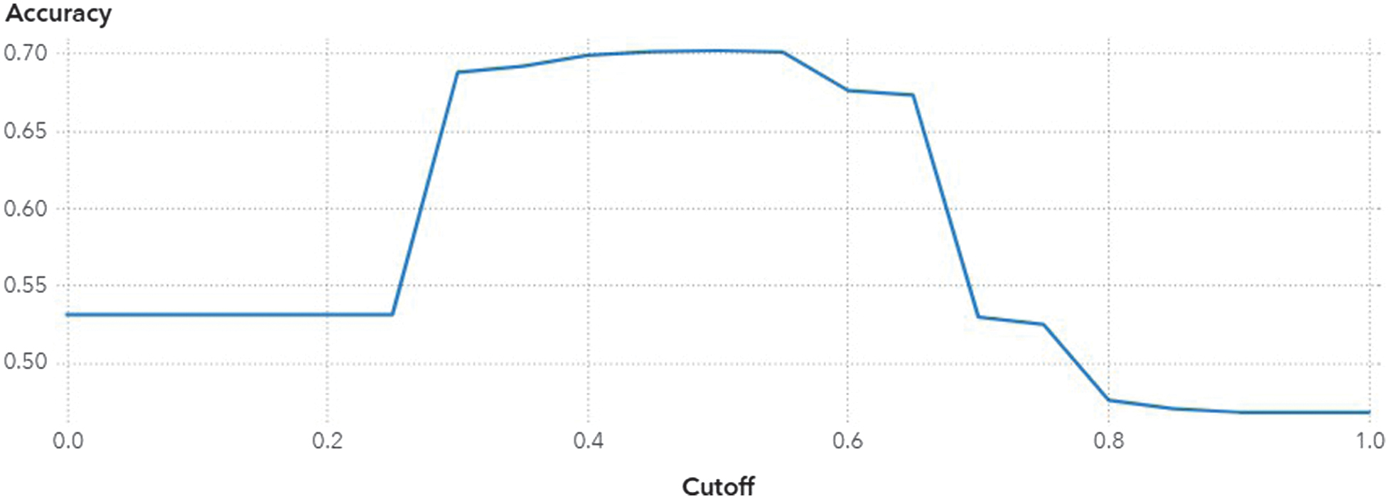
Figure 10 illustrates the impact of cutoff thresholds on the accuracy of classification models. The horizontal axis displays cutoff values ranging from 0.0 to 1.0. The accuracy of each threshold is represented vertically. This plot evaluates the equilibrium between correct predictions for both positive and negative classes to identify the threshold that yields optimal classification performance. The precision ranges from 0.50 to 0.55 when utilizing low cutoff values between 0.0 and 0.2. This range indicates that the model fails to capture numerous instances, probably due to an overestimation of positive predictions. As the cutoff exceeds 0.2, there is a rapid increase in accuracy, which stabilizes between 0.35 and 0.65, reaching a maximum at 0.70. The equilibrium between true positives and true negatives positions this plateau as the optimal threshold zone for predictive accuracy in the model. Following 0.6, there is a gradual decline in accuracy, which accelerates rapidly after reaching 0.7. This decline suggests that the model is adopting a more conservative approach, accurately identifying fewer positive cases while resulting in a rise in false negatives. Once more, accuracy stabilizes around 0.50 as the threshold nears 1.0. The model’s performance is nearing that of random classification. Figure 11 demonstrates the impact of the cutoff threshold on the performance of the model. The optimal cutoff range, typically between 0.35 and 0.6, effectively balances sensitivity and specificity to ensure precise predictions. This analysis is particularly valuable for evaluating risks, detecting fraud, and diagnosing medical conditions, as selecting the appropriate decision threshold significantly influences classification outcomes.
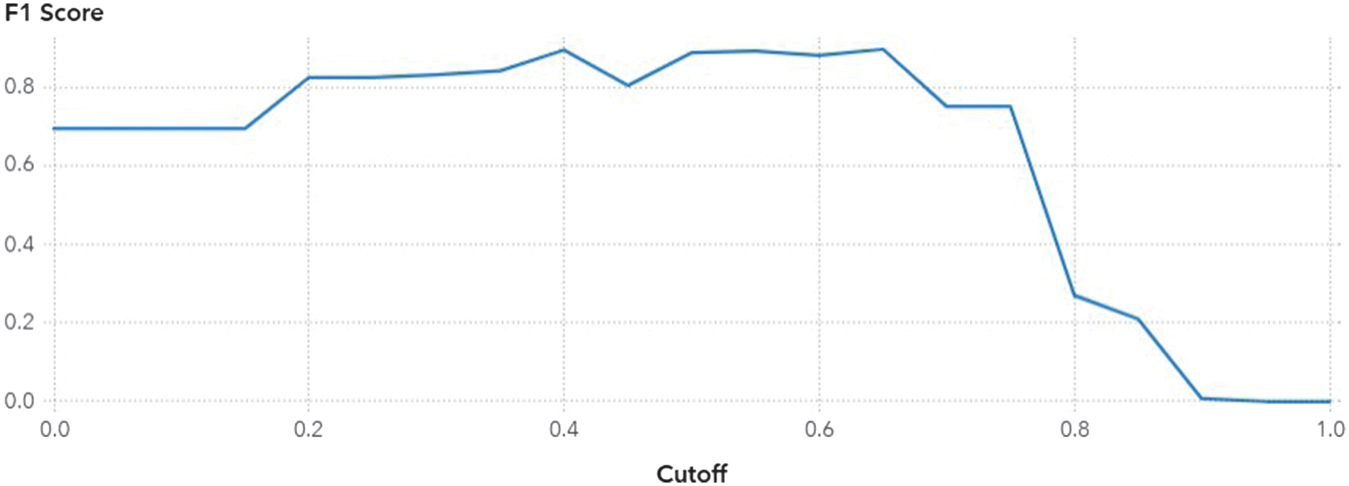
Figure 11 illustrates the relationship between the F1-score of the binary classification model and the cutoff threshold. The vertical axis represents the harmonic mean of precision and recall, known as the F1-score. The horizontal axis displays cutoff values ranging from 0.0 to 1.0. This metric effectively evaluates the model’s ability to identify positive instances while minimizing both false positives and false negatives. The F1-score ranges from 0.65 to 0.70 for low cutoff values between 0.0 and 0.2. Although recall is elevated, precision suffers due to the model identifying an excessive number of instances as positive. Following the adjustment of the cutoff from 0.25 to 0.6, the F1-score remains within the range of 0.85 to 0.90. At this plateau, the model successfully identifies true positives while minimizing false alarms, resulting in optimal performance. The F1-score exhibits a gradual decline beyond 0.6, followed by a more pronounced drop after 0.75. As the value approaches 0.9, the F1-score declines to below 0.3 and nears zero as it gets closer to 1.0. The observed pattern indicates that the decision boundary is increasingly conservative, leading to a reduction in positive outcomes and diminished recall accuracy, despite maintaining high precision in certain instances. Figure 11 illustrates the sensitivity cutoff of the model. The model achieves optimal F1 performance within the range of 0.3 to 0.6. In scenarios where the implications of false positives and negatives are significant, this analysis is essential for establishing a decision threshold that guarantees high predictive accuracy and equitable classification performance.
IV.LONG SHORT-TERM MEMORY (LSTM)
An LSTM was utilized for ABSA in our study. The LSTM model demonstrated exceptional performance in identifying complex emotions linked to particular segments of textual data. The LSTM model attained an accuracy of 66.18 percent, demonstrating its ability to accurately predict outcomes for roughly 65.18 percent of the instances in the test set. Figure 12 presents the accuracy, sensitivity, and F1-measure obtained for each classification category in the GRU model.
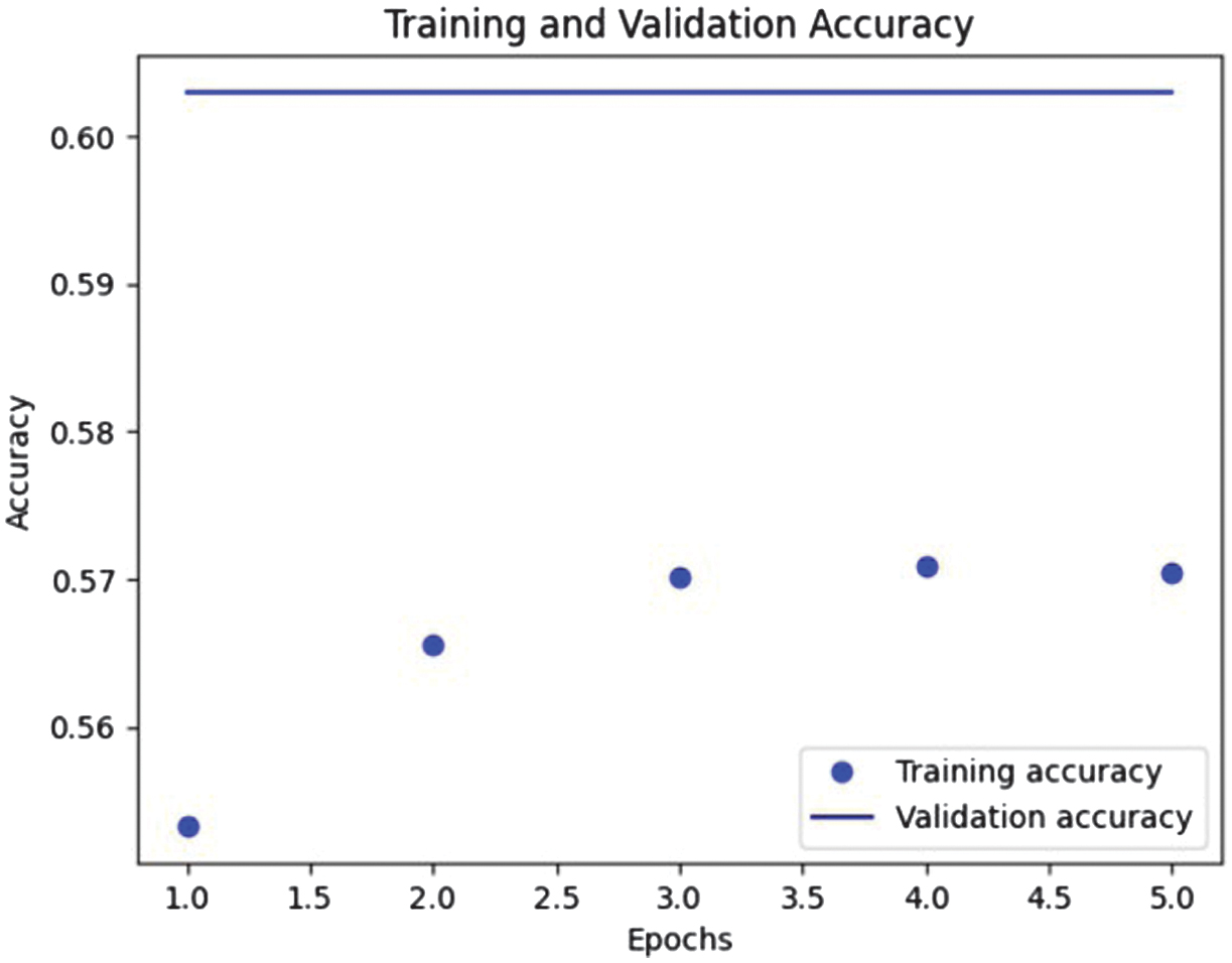 Fig. 12. Accuracy of GRU model.
In the positive class, if we consider all instances to be positive, it turns out that 52% are truly positive, which is reflected in a precision value of 0.52. A recall score of 0.45 signifies that the model successfully recognizes 45% of actual positive occurrences. The F1-score, which is determined by the harmonic mean of recall and precision, stands at 0.49. The evaluation provides a comprehensive analysis for the positive category.
The model forecasts the negative class around 70% of the time, resulting in a precision of 0.70. The model successfully identifies 84% of the true negative instances, as reflected by a recall of 0.84. The F1-score of 0.76 for the negative class indicates a well-rounded evaluation of both recall and precision.
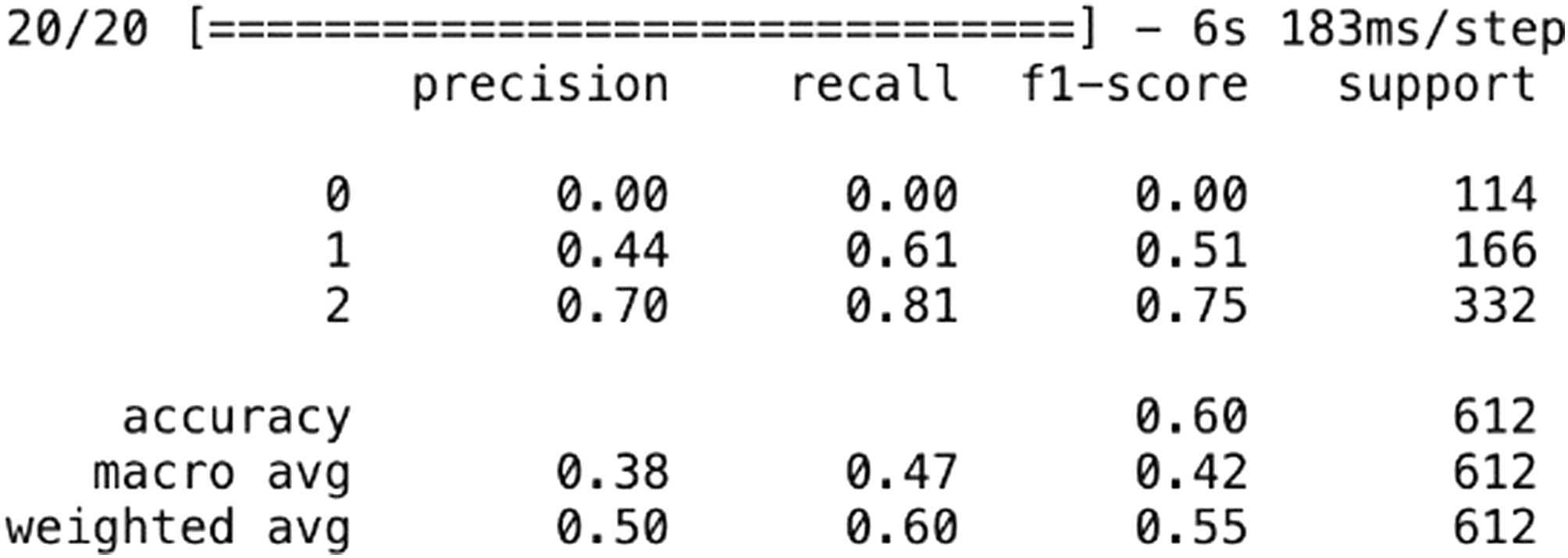
The neutral class demonstrates that 71% of instances predicted as neutral are accurately classified, indicating a precision of 0.71 for this category. The model effectively recognizes 70% of the authentic neutral instances, as demonstrated by a recall of 0.70. The harmonic mean of recall and precision for the neutral class yields an F1-score of 0.71. The GRU model achieves an accuracy of 60%.
A.PERFORMANCE METRIC
Figure 13 illustrates the model’s impressive F1-score, recall, and precision, indicating its strong performance in Class 2. Class 1 performs about average, with respectable recall and precision, leading to a respectable F1-score. Class 0 exhibits a lack of performance, evidenced by a precision, recall, and F1-score of 0.00. To get a feel for the big picture, the weighted averages and macros should be examined.
V.INTERPRETATION AND PERFORMANCE EVALUATION
In our study, we rigorously evaluated various models to ascertain their performance across multiple metrics. The superior performance of the Bayesian network can be attributed to its probabilistic graphical structure, which explicitly models conditional dependencies between aspects, entities, and contextual variables. In contrast to LSTM and GRU architectures that rely on sequential token learning, BN captures structured inter-variable relationships, which are particularly advantageous in ABSA tasks where entity-aspect polarity interactions are discrete and interpretable. Additionally, the relatively moderate dataset size of SentiHood may limit deep neural architectures from fully generalizing, whereas probabilistic models perform efficiently under limited data conditions.
The Bayesian network emerged as the top-performing algorithm, exhibiting an impressive accuracy of 88% and an F1-score of 0.887 as shown in Table II. Although LR showcased reasonable results with an accuracy of 68% and an F1-score of 0.733, it fell short compared to the Bayesian network. Similarly, GB presented moderate performance with 70% accuracy and an F1-score of 0.746 as shown in Table II. Notably, our RNN models, including LSTM and GRU, portrayed competitive but comparatively lower accuracy as shown in Fig. 14, with LSTM achieving 66.18% accuracy and an F1-score of 0.68, while GRU showcased a lower accuracy of 60% with an F1-score of 0.42. Overall, the Bayesian network stands out as the most accurate and reliable model among those considered in our analysis as shown in Fig. 15.
Table II. Comparison between machine and deep learning algorithms
| Algorithm name | Accuracy | F1-score |
|---|---|---|
| Bayesian network | 88% | 0.887 |
| Logistic regression | 68% | 0.733 |
| Gradient boosting | 70% | 0.746 |
| LSTM | 66.18% | 0.68 |
| GRU | 60% | 0.42 |
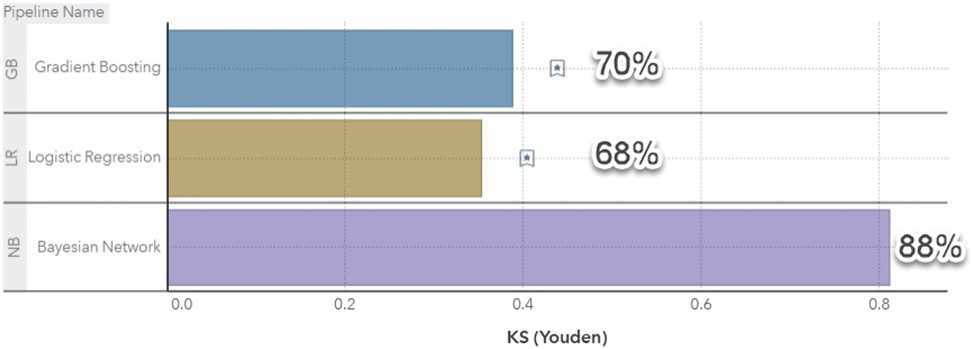 Fig. 14. Assessment for machine learning models.
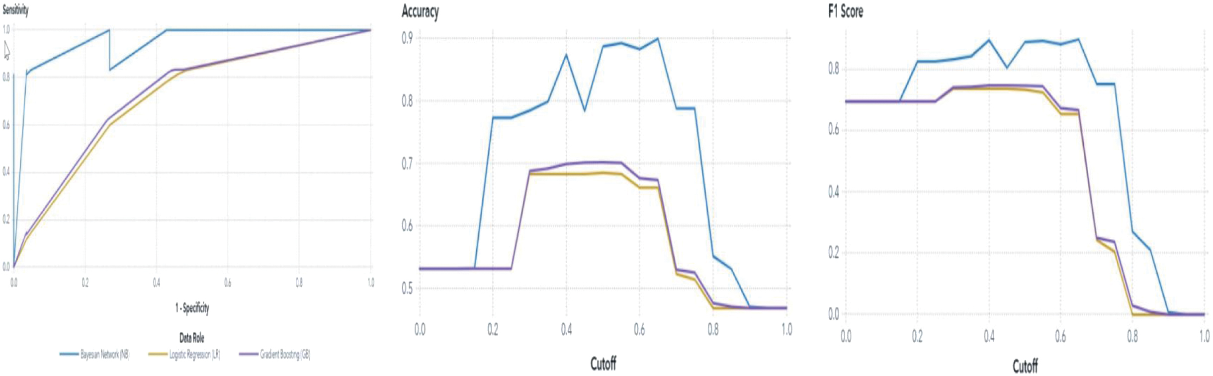 Fig. 15. ROC curve for all machine learning algorithms.
To verify whether the performance improvements were statistically significant, paired t-tests were conducted between the Bayesian network and other models using F1-scores across five cross-validation folds. The results showed statistically significant improvement of BN over LR (p < 0.01), GB (p < 0.01), and LSTM (p < 0.05). Bootstrap resampling (1,000 iterations) further confirmed the robustness of BN’s superior F1 performance, with 95% confidence intervals not overlapping with competing models.
A BERT-base uncased model was fine-tuned for three epochs with learning rate 2e-5 and batch size 16. It achieved 84% accuracy and 0.861 F1-score, slightly below the Bayesian network.
Table III shows an overview of related work detailed in some papers that, like us, include the author, aim, dataset used, algorithm employed, polarity, and results. It offers a concise summary of the different approaches and findings in the field of sentiment analysis, allowing for a quick comparison of the various studies and their contributions to the domain.
Table III. Comparison between related work and our results
| Author | Algorithm | Accuracy | Our accuracy |
|---|---|---|---|
| Logistic regression | 87% | 68% | |
| LSTM | 89% | 66% | |
| Bayesian network/Naive Bayes |
The findings of this current study align with recent advancements in sentiment analysis from 2020 to 2025, which emphasize deep learning, contextual modeling, and domain-specific adaptations. The progress of deep learning models has established that CNNs and LSTMs consistently outperform traditional approaches [22]. In a similar vein, Xu et al. [23] improved ABSA through the use of hierarchical graph attention networks, aiming to more effectively capture dependencies among aspects. Conversely, Gao et al. [24] presented a location-aware sentiment framework that utilizes geotagged tweets to illustrate urban public opinions, which is closely aligned with the direction of this study. Zhang et al. [25] enhanced LSTM-based models for aspect-level sentiment detection, resulting in improved contextual precision. Li et al. [26] utilized BERT to analyze urban tourism reviews, enhancing the identification of feature-level polarity.
Certain theoretical investigations related to this study’s findings suggest that deep contextual embeddings for detailed aspect sentiment extraction, along with attention mechanisms utilizing GRU networks, enhance accuracy in the classification of sentiment on social media [27,28]. In a similar vein, Al-Hassan and Al-Dossari [29] created deep learning models aimed at analyzing sentiment in Arabic tweets, tackling both language and imbalance issues. Qi et al. [30] introduced a novel approach to sentiment analysis in the tourism sector by integrating text and image features, thereby improving interpretability. The work of Nweke and Teh [31] alongside Nguyen et al. [32] has revealed challenges in explainability and resource optimization, as well as in spatial sentiment mining utilizing Twitter data to aid city governance and urban decision-making. This aligns with the focus of the study.
Ultimately, the findings of the present study align with the contributions of Sharma and Dey [33], who enhanced contextual awareness in text interpretation, as well as the research conducted by Ahmed and Hassan [34], which integrated CNN and LSTM architectures for effective sentiment classification on extensive datasets. The comparative results were further substantiated by the findings of Wang et al. [35], who developed attention-guided deep networks that enhanced the precision of fine-grained sentiment detection, alongside the study conducted by Ali and Khan [36], which analyzed the performance of machine learning and deep learning models, concluding that deep learning provided enhanced generalization and scalability. Lastly, the findings of the current study were bolstered by Khalid and Qureshi [37], who introduced Bayesian deep learning for sentiment and opinion mining in location-based reviews, thereby enhancing probabilistic modeling for social and geographical sentiment contexts.
VI.CONCLUSION
This work presents a novel approach for conducting targeted ABSA. This analysis aims to undertake a thorough examination of the sentiments expressed by the general public regarding particular attributes found across diverse geographical locations. The recognition that understanding public opinion is essential for making well-informed decisions in urban planning, tourism development, and the promotion of community involvement is the driving force behind our decision-making process. To facilitate research in this area, we assembled a comprehensive dataset tailored for exploring the emotions linked to different geographical regions. Furthermore, in order to overcome this challenge in an efficient manner, we presented a comprehensive collection of machine learning and deep learning methods. We recognized areas for development, such as utilizing parse trees to better capture the contextual intricacies of each site, despite the fact that our basic models provided a great foundation since they gave a robust foundation with which to build. We conducted a thorough analysis, and the results showed that the Bayesian network was the model that performed the best. It achieved an excellent accuracy rate of 88%. Although our approach primarily utilizes existing machine learning and deep learning models, its contribution is distinctive in its application to geospatial sentiment analysis, particularly within the context of urban neighborhoods. This geographic orientation is relatively underexplored in sentiment analysis literature. The study’s findings support practical applications across city management, tourism strategies, and neighborhood planning, underscoring its value to both academia and practitioners. For instance, in Jeddah, this model could guide municipal planning by identifying neighborhoods with persistent negative sentiments related to safety or transportation. This study demonstrates that probabilistic graphical models are effective in capturing the intricate linkages that exist within geographical sentiment data. Particularly noteworthy is the fact that the Bayesian network outperformed traditional machine learning methods such as LR and GB, in addition to more complex deep learning designs like LSTM and GRU. When addressing complex tasks like targeted ABSA, this conclusion emphasizes the significance of considering a range of modeling methodologies.